Shape determination of unidimensional objects:
the virtual image correlation method
M. Franc¸ois1,a, B. Semin1, H. Auradou1, and J. Vatteville1 1 Laboratoire FAST, Universit´e Paris Sud XI, 91405 Orsay 2 Laboratoire FAST, Universit´e Paris Sud XI, 91405 Orsay 3 Laboratoire FAST, Universit´e Paris Sud XI, 91405 Orsay 4 Laboratoire FAST, Universit´e Paris Sud XI, 91405 Orsay
Abstract. The proposed method, named Virtual Image Correlation, allows one to iden-tify an analytical expression of the shape of a curvilinear object from its image. It uses a virtual beam, whose curvature field is expressed as a truncated mathematical series. The virtual beam width only needs to be close to the physical one; its gray level (in the trans-verse direction) is bell-shaped. The method consists in finding the coefficients of the series for which the correlation between physical and virtual beams is the best. The accuracy and the robustness of the method is shown by the mean of two examples. The first details a Young’s modulus identification from a cantilever beam image. The second is relative to a thermal plume image, that have a weak contrast and a lot of noise.
1 Introduction
”Unidimensional” objects, designated as beam by the mechanician, are of interest in various scientific fields: biology (human hair, blood vessels...), botany (plant stems...) and of course mechanics (beams in solid mechanics, flexible fibers in fluid mechanics...). These objects present a large aspect ratio (from 100 to 1000 in the examples).
The beam mechanics associates the flexural momentum to the curvature field. The method issued from the image processing field (such as skeletonizing, level set methods, ridge following methods [1] or Radon transform based methods [2]) generally provide a set of pixel as a result: due to its roughness, the second derivative can generally not be used as it.
Due to processors and camera improvements, the full-field measurement methods [3, 4] recently took a major role in experimental mechanics. However, they cannot work on unidimensional objects whose width is close to the pixels size. Others aspects prevent to use them: the motion of flexible wires can be many orders larger than their width and the simple shape identification is not possible (because no reference image is available).
The present Virtual Image Correlation (VIC) method uses an image correlation algorithm close to the one used in full-field measurement methods. It consists in finding the best correlation between the physical beam image and a virtual beam. From an approximate initial shape, the virtual beam is gradually ”deformed” until it perfectly matches (with respect to a quadratic distance) the physical beam image.
a e-mail:[email protected]
© Owned by the authors, published by EDP Sciences, 2010 DOI:10.1051/epjconf/20100610004
2 The virtual beam description
The virtual beam is described upon its mean line positionx(s) (sis the curvilinear abscissa), its angles
θ(s) (with respect toe1where (e1,e2) is the reference frame) and curvaturesγ(s). The curvature field
is described by a truncated series:
γ(s)= N X
n=0
Anγ˜n( ˜s). (1)
The tilde terms refer to dimensionless expressions: ˜s∈[0,L] = s/LwhereLis the overall length of the beam. The functions ˜γnare the basis functions of the series description (Lagrange or Fourier in the present case) and the Anare their respective weights. By successive integrations, this equation gives θ(s) and x(s). The virtual beam lightnessl(r), wherer ∈ [−R,R] andR is the radius of the virtual beam, varies like a shifted cosines function whose widthRis chosen slightly larger than the width of the physical beam image.
2l(r)=1+cos πr
R
(2)
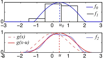
The physical beam mean line is defined from the best correlation between the physical and virtual beam image. The method is detailed in the next section. The bell shape of l(r) gives, for the most of the case studies, a good determination of the mean line as soon as the physical beam lightness increases from the border to the center, even if its width is close to one pixel. Fig. 1 illustrates the method, in an uni-dimensional point of view (the sketch can be seen as a cross section of the beam). The function f0models a physical lightness of the object: its symmetry axis is set atu0=0.4 (pixels).
The function f1 represents its discretization over the pixels of the camera. The virtual beam
bell-shaped function is g(x); it is discretized over a fine grid (here 0.1 pixel). Its shape and width are different from f0(x). The function f2is the cubic interpolation of f1 over the fine grid ofg. The best
correlationR(f2(x)−g(x−u))2dxis (numerically) obtained for the shift u = 0.378 pixels. Despite
the raw discretization and the different functions f and g, the correlation method provides a good identification of the mean line, at the sub-pixel scale.
−3 −2 −1 0 1 2 3
0 1
−3 −2 −1 0 1 2 3
0 1
f0
f1
f2
g(x) g(x-u)
u0
u
Fig. 1.1D sketch of the method
3 The optimization method
The researched parameters are the coefficientsAk of the series and the two integration constantsθ0 andx0 (the values ofθandxfor the initial point). This last one is reduced to one of its component,
herex0,2, in order to fix the curvilinear abscissa of the beam (else the problem is underdefined). These
terms are joined together in a pseudo vectorVk={x0,2, θ0,Ak}: the optimization consists in finding the minimum, overVkof the functionΦdefined as:
Φ= "
Dg
that is the correlation between the virtual (g) and physical (f) beam images. Writing the condition of minimum∂Φ/∂Vk=0 (and consideringg(X), whereX(Vk) represents the current point of the virtual beam) gives:
I
∂Dg
(f−g)2n.∂X ∂Vk
dVk !
dl−2 "
Dg
(f −g) grad(g).∂X
∂Vk dVk
!
dS =0. (4)
The first (boundary) term, in whichnis the outer normal vector, is neglected on the two (small) ends of the beam ats=0 ands=L. Its value over the lateral borders (r=±R) can be also neglected if one supposes that f, at these points (in the background of the physical image), is a constant value f|∂Dg.
Sinceg(±R)=0 (see Eq. 2), using the divergence theorem leads to: I
∂Dg
(f−g)2n.∂X ∂Vk
dVk dl=(f|∂Dg)
2 ∂ ∂Vk
" Dg
div(X)dS
dVk. (5) As div(X) is constant (equals 2), the right hand term equals to zero and the optimization condition
(Eq. 4) reduces to: "
Dg
(f −g) grad(g).∂X
∂Vk !
dS =0. (6)
The analytical definition ofgallow a simple calculus (and fast computation) ofgrad(g) and∂X/∂Vk that is detailed hereafter. Following [4], this equation is discretized in order to use a Newton iterative process:
g(Vk+∆Vk)=g(Vk)+grad(g). ∂X ∂Vp
∆Vp. (7)
This, with Eq. (6), gives:
∆Vp "
Dg
grad(g).∂X
∂Vk !
grad(g).∂X
∂Vp !
dS =
"
Dg
grad(g).∂X
∂Vk !
(f−g)dS, (8) wich is a simple matrix equation, that can be rewritten as Mk p∆Vp = Lk. Its solution∆Vp defines the updated shape of the virtual beam. The iterative process stops with respect to a speed convergence criterion. The computation off−grequires the projection offon the generally thinner and curvilinear frame ofg; this is done by using a cubic interpolation.
The termgrad(g).∂X/∂Vkis involved in both the expressions ofMk pandLk. From Eq. (2) and the beam geometry follows:
grad(g)=l0(r)ν, (9) and, considering thatX=x+rν:
∂X ∂Vk
= ∂∂x
Vk
−r ∂θ
∂Vk
τ. (10)
The second term, collinear toτ, does not need to be computed as it is orthogonal tograd(g). Denoting as ˜θnthe primitive of ˜γnthe derivatives of∂x/∂Vkare:
∂x ∂x0,1
=e1, ∂x ∂x0,2
=e2, ∂x ∂θ0
=Z s 0
νdξ, ∂x
∂An =L
Z s
0
˜
θnνdξ. (11)
The displacement of the virtual beam between two steps is close to (∂X/∂Vk)∆Vk where the fields ∂X/∂Vkrepresent unitary kinematic fields. Figure 2 shows an example of such fields (for clarity the fields are only represented at the mean line location, i.e.∂x/∂Vk). They play the same role as the unitary displacement fields used in the DIC method [4].
The virtual image G is naturally discretized over the curvilinear frame (s,r) that does not corre-spond to the square grid of image F. To avoid any loss of information, the mesh size of the virtual image is much smaller. The computation of the second member of Eq. (8) requires one to project the luminance field f onto the mesh of G using, here, a cubic interpolation.
Fig. 2.Examples of unitary displacement fields. From left to right:∂x/∂x0,2(vertical translation),∂x/∂θ0(rotation) and∂x/∂A0(uniform increase of the curvature).
4 Raw identification
0
50
100
150
200
100
200
300
0
(a)
60
70
100
110
50
(b)Fig. 3.Preliminary identification: (a) full picture, (b) detail of the loop (pixels)
The previous calculus (precisely the transformation from Eq. 4 to Eq. 6) supposes that the virtual beam already contains the physical beam image. A preliminary shape identification is done. It consists of a discrete version of the Virtual Image Correlation method, in which the virtual beam reduces to a straight segment (of typical length 4R) whose kinematic field is the sole rotation around its first extremity. The segment centers are retained as beam points. This method has proven to be robust and able to deal with loops: at the crossing points, the weight of the pixels belonging to the other branch branch tend to compensate each other. Fig 3 illustrates such preliminary identification. The image is extracted from a film of a thin fiber moved by a fluid flow in a transparent fracture [5]. No preliminary image treatment was done; the image is used in inverse video. On this ill-defined image, the radius of the virtual beam was set atR=1 pixel. The computing time is a few seconds.
5 Influence of the series order
From the rough identification are computed the corresponding parameters Ak for an order N0 that
equals the number of segments (this calculus is not detailed here). The user can choose another one for the precise identification: initial values are obtained either by truncatingAkif the chosen orderN<N0
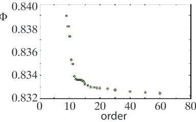
or by filling it by zeros in the opposite case. Fig. 4 shows the result of the identification, for a Fourier series withN=80: the virtual beam perfectly matches the physical one, even in the detail view. Due to the analytical definition of the virtual beam, this shape remains smooth (and infinitely derivable). The precision of the identification depends uponN: Fig. 5 shows the evolution of the correlation function
100
150
50
100 150 200
(a) (b)
Fig. 4.Identified shape forN=80. (a) global view. (b) detail of the loop.
match the physical shape. ForN > 8,Φ decreases withN. Tests have proven independence of the result with respect to the history of the order choices.
order
Φ
0.832
0.834
0.836
0.838
0.840
10
20
40
60
80
0
Fig. 5.Correlation with respect to the series orderN.
6 Exemple: identification of the Young modulus of a straight beam
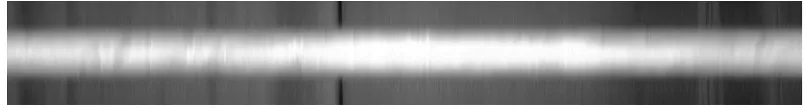
A 2017-T4 aluminium straight bar (diameter 4.95 mm, length 2459 mm) has been fixed in the horizon-tal chuck of a milling machine in front of a black curtain. It bends under its own weight. The proposed method provides the shape, slopes and the curvatures of the bar. This last one has a strong mechanical meaning in the Timoshenko’s beam theory as it is related to the bending moment. Considering that the external actions only reduces to the gravity, the beam theory writes as:
M(s)= Z L
s
ρ(x1(ξ)−x1(s)) dξ, (12)
M(s)=EπR
4
4 γ(s), (13)
θ(0)=0, (14)
in whichMis the flexural moment,ρ=2700 kg/m3the density,Ethe Young modulus andx
1denotes
the horizontal axis. In the large transformation framework, this problem accepts a numerical solution that is compared to the measurement obtained by our technique. The criterion retained for comparison is the least square distance between the the ordinatesx2. The best fit was obtained forE = 72 GPa,
Fig. 6.Aluminium bar bending under its own weight.
0
-0.2
-0.4 x2
L
0 0.5 xL1
(a) 10-3
-10-3
0
0 0.5 1sL
∆x2 L
(b) Fig. 7.Displacements. (a) Timoshenko theory (solid line) and VIC identification (circles). (b) ordinates discrep-ancy between the Timoshenko and VIC results.
which the chuck was rotated of an half tour, shown that this was comparable to the imperfect straight-ness of the beam. The optical aberrations, other possible source of errors, were not compensated in that study. The identification was done with a Legendre series withN = 8. The choice of the order
Fig. 8.The aluminium bar seen in the unwrapped frame of the virtual beam.
7 Example: thermal plume boundary identification
c
b
(a)
500 520
480 250
270 290
540 310
460
240
230
220 120 130 140 150
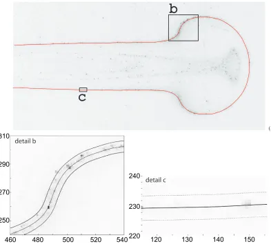
Fig. 9.Thermal plume (inverse video). a) physical image and identification (continuous red line), b) and c) details (pixels), external line: borders of the virtual beam.
The figure (9a) represents a thermal plume picture (344x719 pixels): the fluid (sugar sirup) is heated by a circular device on the bottom of the reservoir. This experiment is similar to the thermal plume existing in the earth mantle. The markers are thermochromic liquid crystals which brighten at a given temperature (23.4◦C on this example). The analytical shape of the plume is required for further studies on this Rayleigh-B´enard convection mechanism. The external contour of the plume is represented by a discontinuous collection of pixels, whose luminance vary in a large amount; for example, the figure (9c) shows a domain with very weak luminosity and a discontinuity of the physical pixel line. Various image processing methods have been tried without success on this picture. The raw identification method detailed in Sec 4 proves here its robustness.
discretization). OrdersNsuch asN≥40 give successful identifications; the corresponding correlation distances varies fromΦ(N=40)=32.1% toΦ(N=168)=31.6%.
8 Conclusions
The proposed method is shown to be accurate and robust with respect to image noise and even loops. It does not require any preliminary image processing. The computation time remains of the order of the minute, within the Matlab environment, a current computer and high-resolution digital image. The method takes into account all the pixels of the physical beam image but does not use the rest of the pixels that constitutes, in general, a large amount of the image. Furthermore, this makes the method naturally insensible to large artifacts in the background (such as stones in Fig. 6).
A future development will consist in the determination of the local flexural stiffness of beam and wires by using two pictures that differ in the gravity direction. This should apply for beams whose free shape is unknown (on the contrary of the example in Sec 6). Other development may concern images sequences, in which the identified shape parameters of an image will be used as a first evaluation for the next image. Three dimensional development is also envisaged, with the use of two cameras. Finally, the method can be easily adapted for the contour identification problem by the use of a step-shaped virtual beam lightness.
9 References
References
1. Aylward, S. R. and Bulitt, E., IEEE Transactions on Medical Imaging21, (2002) 61-75 2. Toft, P. A., Proceedings of the IEEE ICASSP-96 Conference4, (1996) 2219-2222
3. Gr´ediac, M. and Toussaint, E. and Pierron, F., Int. J. of Solids and Structures39, (2002) 2691-2705 4. Hild, F. and Roux, S., Strain42, (2006) 69-80