R E S E A R C H
Open Access
Smartphone-based outlier detection: a
complex event processing approach for
driving behavior detection
Igor Vasconcelos
1,2*, Rafael Oliveira Vasconcelos
1,2, Bruno Olivieri
1, Marcos Roriz
1, Markus Endler
1and Methanias Colaço Junior
3Abstract
The majority of fatal car crashes are caused by reckless driving. With the sophistication of vehicle instrumentation, reckless maneuvers, such as abrupt turns, acceleration, and deceleration, can now be accurately detected by analyzing data related to the driver-vehicle interactions. Such analysis usually requires very specific in-vehicle hardware and infrastructure sensors (e.g. loop detectors and radars), which can be costly. Hence, in this paper, we investigated if off-the-shelf smartphones can be used to online detect and classify the driver’s behavior in near real-time. To do so, we first modeled and performed an intrinsic evaluation to assess the performance of three outlier detection algorithms formulated as a data stream processing network which receives as input and processes data streams of smartphone and vehicle sensors. Next, we implemented a novel scoring mechanism based on online outlier detection to quantitatively evaluate drivers’maneuvers as either cautious or reckless. Thus, we adapted a data mining mechanism which takes into account a sensor’s data rates and power to determine driver behavior in the scoring process. Finally, as the intrinsic evaluation does not necessarily reveal how well an algorithm will perform in a real-world scenario, we evaluated the algorithm that achieved the best result in a real-world case study to assess drivers’driving behavior. Our results indicate that the algorithm performs quickly and accurately; the algorithm classifies driver behavior with 95.45% accuracy. Moreover, such results are obtained within 100 milliseconds of processing time on average.
Keywords:Online driving behavior detection, Online outlier detection, In-Vehicle sensing, Smartphone
1 Introduction
Driving is an everyday task that has become a necessity for modern society, primarily in large cities. According to Owsley [1], in some cases driving is associated with quality of life. However, reckless driving has caused a growing number of traffic accidents. Reckless driving is defined as driving behavior defined by Tasca [2] as behavior that “de-liberately increases the risk of collision and is motivated by impatience, annoyance, hostility or an attempt to save time.” According to a global safety report traffic by the World Health Organization [3], 1.24 million people die each year in traffic deaths and an estimated 20–50 million
are involved in non-fatal accidents. In addition, it is esti-mated that $518 billion dollars is spent on the conse-quences of accidents [4]. However, studies indicate that drivers tend to be relatively safer when monitored or when feedback on their maneuvers is provided [5, 6].
Nevertheless, current intelligent transportation sys-tems (ITS) continue to rely on an infrastructure com-posed of static sensors and cameras installed on roads, making it difficult to collect, aggregate, and analyze data, especially in real-time [7–9]. Moreover, due to the high cost of installation and maintenance, ITS are often re-stricted to particular roads or neighborhoods [9–11]. By contrast, the Internet of Things (IoT) aims to pervasively connect billions [12] of things or smart objects such as vehicles, sensors, actuators, and smartphones. The IoT poses a more complicated challenge in multi-stream en-vironments where multiple data streams compete for available memory and processing resources, especially in
* Correspondence:[email protected] 1
Department of Informatics, Pontifical Catholic University of Rio de Janeiro (PUC-Rio), Rua Marques de São Vicente 225, Gávea, Office 503, Rio de Janeiro-RJ, Brazil
2Department of Informatics, University Tiradentes (UNIT), Aracaju, Brazil
Full list of author information is available at the end of the article
resource-constrained systems such as sensors and mo-bile devices [13]. For this reason, several IoT solution-s—including tools for safe driving analysis—have been designed and developed to perform data processing in a cloud environment, due to a cloud’s virtually unlimited capabilities and resources in terms of storage and pro-cessing power. For instance, Quintero, Lopez, and Cuervo [14] proposed an approach to classify driving be-havior by collecting data onboard the vehicle and for-warding them for processing in the cloud. Leng and Zhao [15] and He, Yan and Xu [16] proposed a cloud computing middleware for the so-calledInternet of Vehi-cles. However, due to the large volume of data generated by some mobile smart device (i.e., sensors in vehicles), it has become impractical and costly to transmit all data to a cloud [17]. Among the many challenges of the IoT, such as heterogeneity and interoperability, the authors of [18] also highlighted the following: (i) middleware for communication with the cloud [19]; (ii) technologies supporting dynamic configuration [20]; and (iii) robust, real-time mechanisms for data filtering and data mining to cope with the large amount of raw data provided by smart devices and reduce the amount of data transmit-ted to the cloud.
Therefore, mining and processing mobile data streams are a key technique for real-time data analysis [21]. In this scenario, a mobile device is used to receive and analyze a vehicle’s sensor’s data stream such as speed and rotation readings rather than sending these data streams for analysis in the cloud. Furthermore, with this approach, the mobile device can also use its own sen-sor’s data streams—accelerometer and gyroscope read-ings—to enrich the vehicle’s data stream and analyze driver behavior. We argue that analysis of driving behav-ior using the received data streams can be mapped to
the outlier detection problem which refers to the prob-lem of finding data patterns that do not conform to (or deviate sufficiently from) expected behaviors [22, 23], e.g., sudden lane changes and hard breaks. Although outlier detection has been widely studied, little research has been done on detecting outliers in dynamic data streams on mobile platforms. Given thatdynamicmeans a non-stationary context, the pattern discovery algorithm must adapt to the available data streams. For instance, approaches for modeling and recognizing driving behav-ior assume a fixed set of data extracted from onboard vehicle sensors. However, in a real-world scenario, mod-eled sensors may not be available in a specific type/make of vehicle. For instance, most automobile manufacturers have introduced, in addition to the original, standard on-board diagnostics (OBD-II) [24], another set of sensor data such as steering wheel angle, breaks, airbag triggers, [24, 25] and stability control. Thus, the format of ve-hicular sensor reading and the available data depends on either the manufacturer or the vehicle [26]. The outlier detection algorithm must precisely perform within the limited computational resources of mobile smart de-vices, in contrast to the virtually unlimited cloud envir-onment. Moreover, the outlier detection algorithm must operate online, continually processing data items as they are delivered in the input buffer. In contrast, offline al-gorithms require the complete and finite set of input data for processing. Offline algorithms usually buffer all the input data as a batch before processing them. Conse-quently, in offline algorithms the detection of a pattern is delayed until the buffer is filled [27].
With the goal of enabling online detection of reckless driving behavior, this paper investigates online outlier detection algorithms for dynamic data streams on mo-bile devices with limited computational resources. It is
important to highlight that these algorithms need to adapt to the available vehicle’s sensors or mobile device’s sensors. Our study adapts and compares three classical offline outlier detection algorithms to perform online data stream processing using the Complex Event Pro-cessing (CEP) [28, 29] paradigm. Thus, we propose and
evaluate a lightweight approach for detecting outliers through CEP in dynamic data streams generated from mobile devices’ sensors and the vehicle’s onboard sen-sors. Such an approach should (i) perform online data stream mining to identify outliers while respecting the intrinsic computational and storage limitations of mobile devices, and (ii) be able to adapt to the available input data (i.e., sensors) streams. Specifically, the main contri-butions of this research include a mechanism to perform online outlier detection over multiple data streams in a resource-constrained device, and a prototype application that implements these requirements to classify driving behavior. A case study was carried out in a real-world scenario in Brazil with the aim of validating the proto-type. The results indicate a fast (i.e. ~100 milliseconds of processing time) and accurate (i.e., 95.45% accurate) performance.
1.1 Problem statement
Outlier detection refers to finding patterns in data that do not conform to expected behavior [23]. An outlier commonly contains useful information about abnormal characteristics of the system or entity [30]. Outlier de-tection is a multidisciplinary field of study that investi-gates how to extract patterns from large datasets covering a broad spectrum of techniques, such as statis-tical inference, machine learning, and data mining [23, 31, 32]. Moreover, it has been extensively applied in a variety of applications, for instance, detection of finan-cial fraud, network intrusion, failures in critical systems, sensor faults in sensor networks, speech recognition, and traffic monitoring [23, 32].
Despite extensive research on outlier detection, most existing methods require the entire dataset (or at least a large portion of it) to detect outliers [23, 33], and are de-signed to perform offline analysis [22] for a large volume of data. These algorithms have no or only restricted Fig. 2Box plot
support for real-time data analysis requirements - such as meeting timing constraints - and have difficulty adapting to continuous non-stationary data [34]. Online data analytics is particularly significant for applications that need real-time analysis of continuous data streams. This analysis needs to be performed in a manner enab-ling it to run with partial data and with the limited com-putational resources of mobile devices. It is challenging to adapt existing outlier detection solutions to mobile data streams since they were designed and developed for cloud environments with abundant available resources, in which they normally compute with the complete data input [35]. Furthermore, such solutions are treated as a “black boxes” [34], wherein changes can scarcely be made to internal algorithms. The data mining commu-nity has conducted studies addressing outlier detection in data streams; however, these proposals mainly solve difficulties that are not the focus of the current paper, such as clustering [36, 37], mining frequent patterns [38, 39], data analysis [40, 41], and query processing [42] in the cloud environment. The aim of this paper is to in-vestigate online outlier detection over multiple and dy-namic data streams. Moreover, the outlier detection is performed in a smart object with limited processing and storage capabilities (unlike cloud environments) within a mobile scenario in which there is no guarantee that all data will always be available. Based on a systematic re-view of approaches conducted in this paper, we claim that, to the best of our knowledge, the literature offers no solutions to this problem.
A data stream is a continuous and online sequence of unbounded items for which it is not possible to control the order of the produced and processed data [43]. One
characteristic of the data stream is its dynamic nature [44], meaning the properties of data instances may evolve or change over time. Additionally, context changes in a mobile scenario. For instance, it may mod-ify the available data stream’s inputs, and therefore, it is necessary for an algorithm to adapt to the stream’s evo-lution [45]. Recently, online outlier detection within data streams has attracted attention in many constrained emerging applications, such as mobile crowd sensing, mobile activity recognition, ITS, and mobile healthcare [21]. In these applications, multiple and continuous streams are generated by mobile sensors and these streams need to be analyzed in real time. Based on this scenario, it can be seen that the adaptation of strategies for classical outlier detection algorithms to operate with mobile data streams, thus enabling their operation on mobile devices to be efficient, is a challenging research task [21, 35, 46]. This is because (i) outlier detection for data streams is restricted to the partial set of events within a time window; (ii) random access on the set is not possible; (iii) the algorithm must adapt to hardware resources and available sensor data; and (iv) patterns must be discovered within a single pass over the data stream. Moreover, Chandola, Banerjee and Kumar [23] highlight additional factors that make the outlier detec-tion problem more difficult in such a situadetec-tion:
Defining a region encompassing all possible normal
driving behavior is difficult. Furthermore, the threshold between normal and abnormal driving behavior is not often precise. Thus, an outlier observation lying close to the boundary may be normal or abnormal.
Fig. 4An overview of application architecture
The lack of availability of datasets for training and validation is often a major problem. The exact notion of an outlier differs depending on the application domain. An outlier detection
formulation is generated by both the nature of data and the availability of labeled data.
1.2 Motivating scenario
Intelligent transportation systems have received increas-ing attention from academia, industry, and governments, and have been considered the next technological change in individuals’ daily lives [47]. Automobile manufac-turers, in an attempt to overcome the aforementioned ITS limitations, have developed products that help drivers, called Advanced Driver Assistance Systems (ADAS). These systems [48, 49] obtain vehicle data from sensors or embedded devices (e.g., cameras and stability control sensors) for the prevention and detection of col-lisions (e.g., crash sensors can activate airbags), assisted driving, and the generation of offline driving reports. The advantages of ADAS include the rare occurrence of false positives [50] when accessing sensors and devices that are embedded in the vehicle. However, the key im-pediment of ADAS lies in the fact that they are typically available only in new and high-standard vehicles that have prohibitive prices for most drivers [50–52], even in developed countries. Furthermore, the installation of ADAS in older car models is either impossible or inor-dinately expensive. Finally, when ADAS become obso-lete, upgrading or changing to a newer, more efficient system is a difficult task [50], and exorbitant for most drivers.
By contrast, studies have proposed the use of smart-phones to understand and evaluate a driver’s behavior [5, 26, 49, 53–57]. The choice of using a smartphone is made due to its affordability and wide adoption, suffi-cient storage capacity and processing power, as well as its equipment with a variety of sensors. Moreover, a smartphone can act as a processing hub that receives and analyzes data from different vehicle sensors. For in-stance, with Bluetooth, a smartphone is able to connect and receive data from multiple in-vehicle sensors using the OBD-II standard, simultaneously receiving and pro-cessing speed and accelerometer data streams. Further-more, in-vehicle sensors’data streams can be combined with smartphone-embedded sensors (such as direction and location) to further enrich the analysis. Finally, smartphones allow for the development of ubiquitous and loosely connected systems that provide rich data for the analysis of driving behavior.
Currently, approaches that evaluate driving behavior in general use models and techniques (e.g., Neural Net-works, Fuzzy Theory, and Hidden Markov models) with good accuracy [58]. However, they were not designed for data stream processing [40], and according to Lin et al. and Wang, Xi, and Chen [58, 59], have low processing performances, require a long training phase, artificial as-sumptions, or prior knowledge to formulate rules. More-over, since these approaches are statics (i.e., non-adaptable), they have difficulty quickly and accurately recognizing parameters [58], for instance, neural net-works have subjective methods for adjusting the top-ology (number of layers and neurons) and require a fixed number of input parameters. A final drawback, highlighted by Wang [59], is that these approaches are Fig. 6Z-score computation expressed in event processing language (EPL)
“black boxes” with little ability to identify causal rela-tionships making it impossible to understand physical behaviors. However, driving conditions (which are influ-enced by the state of the driver, traffic, and weather con-ditions) are dynamic and as such, all information that a technique or algorithm needs as an input will not always be available onboard. Thus, we believe that an assess-ment of a driver’s driving behavior would benefit from an online outlier detection approach in dynamic mobile data streams.
1.3 Assumptions
This paper considers the following assumptions.
Most data instances in data stream are normal. Only a
small portion of the data consists of outliers [60,61].
Outliers are statistically different from normal data
[2,62].
Battery power consumption is not a critical
requirement because in a vehicle a smartphone can be charged easily when necessary.
However, it is important to note that the first two as-sumptions complement themselves. Considering only the first assumption, some outliers may have behaviors similar to normal data. The second assumption, how-ever, states that outliers are a set of data with behaviors that differ from normal data.
The remainder of the paper is organized as follows. Section 2 presents an overview of the key concepts and system modeling used throughout this work. Section 3 details the proposed approach to online outlier detection for mobile, dynamic data stream. Section 4 highlights definitions and planning of the case study. Section 5 summarizes the main results of the assessment con-ducted to evaluate the proposal. Section 6 discusses
related work. Finally, Section 7 reviews and discusses the central ideas presented in this paper and proposes paths for future work on the subject.
2 Fundamentals
This section presents the main concepts of complex event processing, as well as outlier detection algorithms.
2.1 Complex event processing
Complex event processing (CEP) is a set of tech-niques and tools that provides an in-memory process-ing model for an asynchronous data stream in real time (i.e., minimum delay) for online detection of sit-uations of interest [28]. Complex event processing of-fers [28]: (i) situation awareness through the use of continuous queries that correlate data from different sensors data streams; (ii) context awareness by subdiv-iding data streams into different views, such as tem-poral windows or key partitions; and (iii) flexibility,
since it can specify events at any time, that is, the specification of events can be dynamically changed while a system is running (i.e., on-the-fly).
The CEP central concept is a declarative event pro-cessing language (EPL) to express event propro-cessing rules (continuous queries and patterns). These rules are based on the event-condition-action triad, and use operators (e.g., logic, counting, temporal, causal, and spatial) on in-put events, searching for correlations, exceptional condi-tions, and the occurrence of patterns. The central task of CEP is to provide mechanisms for event pattern matching, i.e., from hundreds or even thousands of events, to identify significant patterns in the application domain [63]. Event processing and pattern detection are made by so-called event processing agents (EPAs) that process an event’s stream. Essentially, an EPA filter sepa-rates, aggregates, transforms, and synthesizes new com-plex events from simple events. A reckless maneuver (e.g., rapidly turning at a high speed) is an example of a complex event, in so far as it is based on the compos-ition of primitive events, such as acceleration, speed, and wheel direction. To perform the detection of such com-plex events, it is necessary to collect and analyze the data stream generated by various primitive sensors, look-ing for patterns and correlations. To detect the pattern of a maneuver, it is necessary to use an important Fig. 8Q2 calculation
concept of CEP called thetime window(or just window). A window is a temporal context that defines which portions of the input data stream are considered dur-ing the execution of an EPL rule [64], i.e., events in the last 30 s, or a snapshot of such recent events [63]. The most common time window models are the batch and sliding window [64]. The former have a fixed lower bound while the upper bound advances every time a new information item enters the system, that is, the CEP engine buffers and processes all events in a time interval. The latter has a fixed size, however, both lower and upper bounds advance when new items enter the system. In others words, it is a moving batch window. An event processing network (EPN) is a network of interconnected EPAs that im-plement the global processing logic for pattern detec-tion through event processing [29]. In an EPN, EPAs are conceptually connected to each other—output events from one EPA are forwarded and further proc-essed by other EPAs—without regard to the particular kind of underlying communication mechanism for event dissemination.
2.2 Outlier detection
Outlier detection techniques typically assume that out-liers in data are rare compared to normal instances. A variety of outlier detection techniques have been devel-oped in several research communities. Many of these techniques have been specifically developed for specific
application domains, while others are more generic. The techniques explained in this paper are used widely in several research areas for identifying outliers in data. The earliest algorithms used for outlier detection were statistical approaches which assume that normal in-stances occur in high probability regions, while anomal-ies occur in low probability regions. The standard score (more commonly referred to as the Z-score) is a simple statistical technique that enables one-pass computation over a data stream to identify outliers, making different kinds of data comparable and easier to interpret [65]. The Z-score describes a raw score’s location in terms of how far above or below the mean it is when measured in standard deviations [65]. A z-score of 0 means that the raw data instance is equal to the mean. The Z-score is calculated as shown in eq. (1), where Z is the Z-score of a data instance, X stands for the sample value, μstands for the mean of the sampling, and σx stands for the standard deviation of the mean. This computation cre-ates a unitless score that is no longer relcre-ates to the ori-ginal units (e.g., km/h and m/s2) as it measures the number of standard deviation units and therefore can more readily be used for comparisons [66].
Z¼X−μ
σx ð1Þ
According to Heiman [65], a Z-score basically has two components: (1) a sign, positive or negative, indicating Fig. 105-summary box plot data
whether the raw score is above or below the mean; and (2) the absolute Z-score value, indicating the score’s dis-tance from the mean when measured in standard devia-tions. According to Chandola, Banerjee and Kumar [23], all data instances whose Z-score module is greater than 3 are declared an outlier. After computing the Z-score for each data instance, the algorithm calculates the distribution (i.e., the relative frequency of the raw Z-scores of a population or sample). Figure 1 shows a per-fect normal Z-distribution (a.k.a., a standard normal curve). It should be noted that 50% of the scores fall below the mean, 50% fall above the mean, approximately 68% of the distribution is between ±1σx from the mean, and Z-scores higher than +3 and lower than −3 occur less than 1% of the time. If these Z-scores were obtained from driving data, this would imply, for instance, that most of the time a driver maintained a driving behavior without abrupt changes in speed or direction. In cases where outliers are detected, the driver may have con-ducted evasive maneuvers to avoid accidents or indeed behaved recklessly, but the number of outliers would still be insufficient to consider the driver reckless. The
strength of the Z-score arises from the fact that this technique does not require user parameters and outliers are discovered with a single pass over the data stream. However, it is susceptible to the number of data in-stances in the dataset and has a unidimensional nature [32].
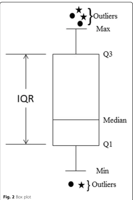
The box plot is likely the simplest statistical technique to detect outliers in both univariate and multivariate data sets that makes no assumptions about the data dis-tribution model [23, 32]. The box plot has become a standard technique for presenting a simple display of a
5-number summary, which consists of the smallest non-anomaly observation (min), lower quartile (Q1), median (Q2), upper quartile (Q3), largest non-anomaly observa-tion (max), and interquartile range (IQR)—the difference
between Q3 and Q1. This means that 25% of observa-tions are smaller than the first quartile, 50% are smaller than the second quartile, and 75% are smaller than the third quartile. Outliers are points beyond the upper and lower values of the box plot [32]. Laurikkala, Juhola and Kentala [67] suggest a heuristic of (1.5 x IQR) beyond the higher and lower values for outliers; however, Fig. 12Computing distance to nearest cluster
according to [32], such a heuristic would need to vary across different datasets. A typical box plot can be seen in Fig. 2. Different from the Z-score, box plots make no assumptions about the data distribution model, however, for multivariate datasets, it is possible to perform a pair-wise distance measure. This technique can have quad-ratic complexity (i.e., in the worst case) since it is founded on the calculation of distances between all data instances [32].
The clustering [68] approach is an exploratory data analysis technique in which a set of input objects,
normally multidimensional, are classified into groups (i.e., clusters) of similar objects. Furthermore, it is essen-tially an unsupervised technique which is preceded by a short and semi-supervised testing and training phase Fig. 14The study route chosen for data collection (map © 2017 Google)
Table 1Confusion matrix
Actual class Predicted class
Positive Negative
Positive True Positive (TP) False Negative (FN)
[30, 69] used to identify outliers. Distance-based cluster-ing approaches use a particular clustercluster-ing measure, such as Euclidian distance. As in the box plot technique, distance-based clustering can have quadratic complexity. Such an approach is based on the following hypothesis according to Chandola, Banerjee and Kumar [23]: nor-mal data instances lie close to their closest cluster cen-troid, while outliers are far away from their closest cluster centroid.
Following the aforementioned hypothesis considering two clusters, as shown in Fig. 3, points P1 and P2 are considered outliers since they are far away from the clusters’centroids. However, as outliers form clusters by themselves, this technique is not able to detect such out-liers because data instances that lie close to a cluster centroid are considered normal data. To overcome this limitation, a second category of clustering relies on the following hypothesis [23]: normal data instances lie close to their closest cluster centroid, while outliers are far away from their closest cluster centroid. Based on this hypothesis, as P1 is closer to the cautious cluster cen-troid, it is considered normal data, while P2is closer to the reckless cluster centroid and thus considered an out-lier. However, it can be extremely costly to collect and label abnormal data [32]. For instance, collecting data that represents reckless driving behavior can even be dangerous, as it may cause traffic accidents. Thus, a clustering algorithm should be capable of identifying outliers with a few data instances that represent reckless driving behavior. For more details regarding outlier de-tection, we encourage readers to refer to [23, 31, 32].
The K-means algorithm is likely the most popular and the widely used unsupervised clustering algorithm [68]
which can classify multidimensional data into different groups on the basis of certain dissimilarity measures. The classical K-means algorithm initially chooses ran-dom cluster prototypes according to a user-defined se-lection process. Next, the input data is applied iteratively and the algorithm identifies the best matching cluster, updating the cluster centroid to reflect the new exem-plar and minimize the sum-of-squares clustering func-tion given by eq. (2), whereμ is the mean of the points (xn) in cluster Sj. However, other distance measurements can be used, such as Euclidean distance [23].
XK
j¼1
X
n∈Sj
xn−μj
2 ð2Þ
Through the combination of EPL rules, it is possible to write algorithms to classify drivers’driving behaviors. Thus, we adapted three outlier detection algorithms to EPL rules to perform online processing of a data stream generated by sensors onboard a vehicle. Sections 3.1, 3.2, and 3.3 explains the algorithms.
3 Related work
Kontaki et al. [70] propose four distance-based algo-rithms for continuous outlier monitoring in data streams. The primary concerns are improving efficiency and reducing memory consumption. To do this, the al-gorithms use the concept of outliers and inliers.A data instance x is considered an outlier if there are less than
kdata instances at a distance, at mostD,fromx, exclud-ingxitself. On the other hand, if the number of data in-stances in theD-neighborhood ofxis enough (i.e., more than k), thenxis characterized as aninlier. To improve
Table 2Performance metrics [83]
Metric Equation
Accuracy is the percentage of instances (evidence) correctly classified. TPþTN
TPþTNþFPþFN
Recall is the percentage of instances that were correctly classified aspositive. TP
TPþFN
Precision is the percentage of instances classified as positive (evidence) that are actuallypositive. TP
TPþFP
F Measure is the harmonic mean of precision and recall, meaning it combines the precision and recall. 2x precisionprecisionþrecallxrecall
Error Rate is the proportion of instances that are incorrectly classified. FPþFN
TPþFNþFPþTN
Table 3Confusion Matrix by Algorithm and Driver (TP and TN)
for h = 100 andΔ= 10
Confusion Matrix
Driver Cautious (True Positive - TP) Reckless (True Negative–TN)
Cluster Box Plot Z-score Cluster Box Plot Z-score
D1 5990 5004 5143 17 49 40
D2 5642 5439 5593 4 52 28
D3 5876 5667 5817 26 75 39
D4 13,465 5618 5716 123 191 45
D5 6114 5024 5201 5 58 41
Table 4Confusion matrix by algorithm and driver (FP and FN)
for h = 100 andΔ= 10
Confusion Matrix
Driver Cautious (False Positive - FP) Reckless (False Negative–FN)
Cluster Box Plot Z-score Cluster Box Plot Z-score
D1 3 19 28 110 175 36
D2 0 34 58 83 201 47
D3 14 40 76 61 191 41
D4 12 14 160 288 131 33
efficiency, the concept of micro-clusters is used to re-duce the number of distance computations. The window size determines the memory size and the number of data instances considered in the time window approach, that is, all data instances in a time window are stored in the main memory and processed by an algorithm. However, the authors control the arrivals and departures of in-stances in the time window. In these events, if the num-ber of neighbors of a given data instance of xis greater thankthen x will never be an outlier and is called asafe inlier. Thus, safe inliers are not stored for further pro-cessing and consequently reduce computation and mem-ory use. Each algorithm has a few variations of this process, however, none have been designed to run on devices with memory and processing constraints.
An online outlier exploration platform, or in short, ONION [71], is proposed for modeling and exploring outliers in large datasets based on a distance-based approach. An ONION employs an offline preprocess-ing phase followed by an online exploration phase, enabling users to establish connections among out-liers. As it is difficult to set appropriate D and k
values [70, 71], the offline phase is a preprocessing three-dimensional phase that computes all possible combinations of D, k, and entire dataset instances. In fact, k can take in the universe of natural numbers and the user must specify lower and upper bounds for k. This phase outputs all outlier candidates. Then, the online phase, with some rules, determines which candidates are actually outliers.
Zhao et al. [55] propose a driver behavior evaluation scoring mechanism named Join Driving (based on the ISO 2631 standard [72]). This mechanism analyzes pas-sengers’comfort level based on their exposure to vibra-tions to classify drivers as cautious or reckless. As human’s feelings in response to vibration depend on the level, frequency, and duration of acceleration, the mech-anism analyzes three-axis accelerometer data. However, because a smartphone is likely in an arbitrary position inside a vehicle, the authors also have developed a novel algorithm for reorientation using GPS and orientation sensor data. The evaluation shows that the mechanism can accurately score driving behaviors in high and mid-value smartphones. The main difference between this approach and those of the current paper is that in Zhao et al. [55] the analysis of the data is offline—performed when a driver reports their arrival arrived at a destina-tion—while our approach is based on online processing, able to help a driver while driving.
To understand and model reckless driving behavior, Hong, Margines and Dey [56] implemented a low-cost, in-vehicle sensing platform. Unlike Zhao et al. [55], which only uses a smartphone’s sensors, this platform added an OBD-II diagnostic device to collect data from the vehicle, such as speed, rpm, speed, and throttle pos-ition. Furthermore, to detect steering wheel movement, a device called an inertial measurement unit (IMU) was added. Both devices communicated via Bluetooth with a smartphone. To characterize driving behavior, a machine learning-based model analyzed data from acceleration
Table 5Algorithm accuracy comparison
Driver h= 100 andΔ= 10 h= 50 andΔ= 20
K-means Box Plot Z-score K-means Box Plot Z-score
D1 98.15% 96.30% 98.78% 98.05% 93.71% 98.58%
D2 98.55% 95.90% 98.17% 98.16% 96.30% 98.80%
D3 98.75% 96.13% 98.04% 98.40% 96.61% 98.59%
D4 97.84% 97.59% 96.76% 96.12% 97.80% 98.94%
D5 98.71% 95.62% 98.63% 97.86% 97.40% 98.57%
Average 98.40% 96.30% 98.07% 97.72% 96.36% 98.70%
Table 6Algorithm precision comparison
Driver h= 100 andΔ= 10 h= 50 andΔ= 20
K-means Box Plot Z-score K-means Box Plot Z-score
D1 99.95% 96.22% 99.46% 99.93% 100.00% 99.52%
D2 100.00% 99.38% 98.97% 99.60% 100.00% 100.00%
D3 99.76% 99.30% 98.71% 99.61% 100.00% 100.00%
D4 99.76% 99.75% 97.28% 99.89% 100.00% 100.00%
D5 99.84% 99.47% 99.16% 99.71% 100.00% 100.00%
Average 99.89% 98.82% 98.72% 99.75% 100.00% 99.90%
Table 7Algorithm recall comparison
h= 100 andΔ= 10 h= 50 andΔ= 20
Driver K-means Box Plot Z-score K-means Box Plot Z-score
D1 98.20% 96,62% 99.30% 98.10% 96.35% 98.91%
D2 98.55% 96.44% 99.17% 98.52% 96.30% 98.80%
D3 98.97% 96.74% 99.30% 98.77% 98.86% 98.60%
D4 97.91% 97.72% 99.43% 96.19% 97.80% 98.94%
D5 98.87% 96.06% 99.45% 98.12% 97.40% 98.63%
Average 98.50% 96.72% 99.33% 97.94% 97.34% 98.78%
Table 8Algorithm F measure comparison
Driver h= 100 andΔ= 10 h= 50 andΔ= 20
K-means Box Plot Z-score K-means Box Plot Z-score
D1 99.07% 98.10% 99.38% 99.00% 98.17% 99.45%
D2 99.27% 97.89% 99.07% 99.06% 98.06% 99.30%
D3 99.37% 98.00% 99.00% 99.19% 98.06% 99.20%
D4 98.90% 98.73% 98.34% 98.00% 99.19% 99.42%
D5 99.35% 97.73% 99.30% 98.91% 98.68% 99.30%
(smartphone sensor), OBD-II, and the IMU. To deter-mine driving behavior, a trip profile is constructed by summarizing trip-profiles obtained from the last three weeks, called driver’s profiles. Finally, the driver’s driving behavior is determined from the driver profile and ma-chine learning. As in the work proposed by Zhao et al. [55], analysis of driver behavior is off-line. However, Hong, Margines and Dey [56], templates must be stored, such as acceleration, deceleration, and curves, which are used for comparison with the driver’s maneuvers and a subsequent classification as cautious or reckless. Accord-ing to Banovic et al. [73], this is a weakness because ma-chine learning algorithms classify and predict only the most frequent behaviors. In this respect, infrequent vari-ations in drivers’behaviors are difficult to detect.
Vehicle data stream mining (VEDAS) [74] aims to iden-tify outliers using a device with low computational power—low processing and storage capacity—and was de-signed to mine a vehicle’s data stream. Data are collected through an OBD-II device and stored in a data stream management system (DSMS) that provides mechanisms to control and access the data through queries. The DSMS provides operators with the ability to compute statistical aggregation such as mean, variance, and covariance. After pre-processing aggregate data, VEDAS constructs a repre-sentation of low dimensional data through three tech-niques: Incremental principal component analysis (PCA), Fourier transformations, or linear online segmentation. Although it is possible to dynamically choose which of the techniques will be used, the authors emphasize that PCA does not work well for online monitoring with limited computational resources. According to the authors, VEDAS implements a collection of techniques and algo-rithms, including proprietary ones, to perform data stream analysis. The authors discuss techniques based on cluster-ing and statistical tests. First, OBD-II data is grouped by
K-means to detect abnormal vehicle health monitoring patterns. The goal of clustering is to identify representa-tions in space that correspond to safe vehicle operation. The detection of unusual driving patterns is performed through acceleration analysis with a linear approximation algorithm, the piecewise linear approximation [75]. In addition, a statistical test is performed on the smoothed data with the algorithm assuming a Gaussian distribution to identify unusual patterns. The data used for validation of the proposal were extracted fromLive For Speed, a driv-ing simulator. However, no driver behavior classification is performed.
The study of Aljaafreh, Alshabatat, and Najim [76] proposes the use of inference by fuzzy logic for online identification of abnormal driving data and driver behav-ior classification based on acceleration and speed. Lat-eral and longitudinal acceleration are categorized in three intervals: low, medium, and high. Speed is catego-rized into five ranges, from very low to very high. The values of these outputs are used to classify drivers’ be-havior. The proposal of Quintero, Lopez, and Cuervo [14] also uses fuzzy logic; however, the output variables are inserted in a neural network properly trained to clas-sify driver behavior. However, the neural network is on a remote server, so all fuzzy system outputs must be sent to this server which performs offline analysis and driver behavior classification. The authors used a backpropaga-tion algorithm, and the best performing architecture was a two-layer neural network, with nine neurons in the intermediate layer and 31 inputs.
4 Online CEP-based outlier detection algorithms This section presents the aforementioned outlier detec-tion algorithms expressed as a set of CEP rules for
Table 9Algorithm execution time comparison
h= 100 andΔ= 10 h= 50 andΔ= 20
Driver K-means Box Plot Z-score K-means Box Plot Z-score
D1 769.6 ms 132.0 ms 100.2 ms 712.0 ms 129.8 ms 98.3 ms
D2 700.0 ms 187.0 ms 103.1 ms 709.4 ms 186.4 ms 99.0 ms
D3 706.4 ms 189.9 ms 100.9 ms 705.5 ms 190.2 ms 99.7 ms
D4 705.3 ms 186.0 ms 101.5 ms 702.3 ms 186.8 ms 100.6 ms
D5 787.0 ms 188.0 ms 102.7 ms 780.4 ms 190.1 ms 100.3 ms
Average 733.6 ms 176.4 ms 101.6 ms 721.9 ms 176.6 ms 99.5 ms
Table 10Smartphone resource consumption
Situation RAM(MB) CPU (%)
Standby 4.53 MB 1.41%
Collecting 5.18 MB 3.60%
Table 11Algorithm resource consumption
Algorithm h= 100 andΔ= 10 h= 50 andΔ= 20
RAM(MB) CPU (%) RAM(MB) CPU (%)
K-means 6.75 MB 20.20% 7.83 MB 23.35%
Box Plot 6.30 MB 11.40% 7.30 MB 11.45%
online outlier detection to operate over a multiple mo-bile data stream, enabling their efficient operation on mobile devices. The algorithms are generic, however, as highlighted by Chandola, Banerjee, and Kumar [23], the exact notion of “outlierness”differs according to the ap-plication domain. Therefore, in our case study, we aim to classify driver behavior based on outlier detection. Our driving behavior characterization algorithms are based on a pattern-recognition approach. Although the modeling relies on an idea proposed by Zhang [77], the difference between the proposals is the fact that Zhang’s work aims to identify the driver’s skill level (e.g., expert or novice) through receiving driver behavior measure-ments as input. Our research aims to identify driver be-havior based on online outlier detection through measurements of the signals from different sensors em-bedded onboard the vehicle, as well as sensors of the mobile device onboard the vehicle.
The processing workflow begins with the interaction between the driver and the vehicle. Each driver exhibits behaviors that can be divided into two types, namely short-term and long-term driving behaviors. The former concerns drivers’instantaneous behavior that should be taken into account separately, such as pressing the accel-erator or the brake. The latter represents larger driving maneuvers, such as making a turn. In this case, it is ne-cessary to consider several issues, namely how the driver accelerates or brakes, the steering wheel angle, and the
driver’s speed [78]. From these behavior types, it is pos-sible to detect a unique driving pattern for each driver, enabling the formulation of a profile representing the driver’s behavior [78].
To sense data from the driving behavior, the stream module is responsible for discovering, connecting, and reading both onboard vehicle and built-in mobile device sensors. This module is able to communicate with on-board sensors via short-range wireless communication technologies, such as Bluetooth and Bluetooth Low En-ergy. More details are available in our previous work [79]. This module acts as a hub and forwards the data stream to the CEP engine for preprocessing. This raw data preprocessing consists in producing higher-level data (referred in this paper asevidence) that best repre-sent the driver behavior. This process is known as fea-ture extraction. A feature is a measurable property that best represent a phenomenon and feature extraction is the processes of deriving the values of such features [80]. As discussed, to measure long-term driver’s behav-ior, some available features need to be analyzed and cor-related over a time period. These features include speed (S = [s1, s2, …, sn]T) and acceleration (A = [a1, a2, …,
an]T). The parameter n denotes the number of instant-aneous sampled values and T denotes a specific time period. Additional features, such as mean speed exclud-ing stops, mean acceleration, mean deceleration, both acceleration/deceleration changes, yaw, and a combin-ation of other physical measurements may be used to measure a driver’s behavior, as discussed in [80].
The online outlier detection module is responsible for finding patterns in the available evidence that deviate sufficiently from expected behavior. The online outlier detection algorithm adapted for CEP rules runs in this module. An important feature of any outlier detection algorithm is the manner in which outliers are reported [23]. On one hand, scoring algorithms, such as Z-scores, assign a score to each evidence estimating the “ outlier-ness”. On the other hand, label algorithms, such as box
plots, assign a label (normal or outlier) to each evidence.
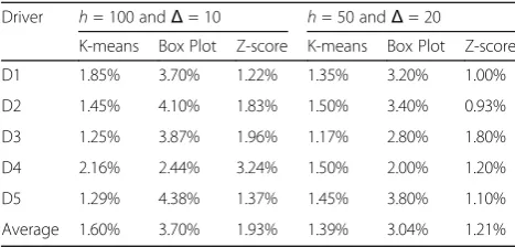
Table 12Algorithm error rate
Driver h= 100 andΔ= 10 h= 50 andΔ= 20
K-means Box Plot Z-score K-means Box Plot Z-score
D1 1.85% 3.70% 1.22% 1.35% 3.20% 1.00%
D2 1.45% 4.10% 1.83% 1.50% 3.40% 0.93%
D3 1.25% 3.87% 1.96% 1.17% 2.80% 1.80%
D4 2.16% 2.44% 3.24% 1.50% 2.00% 1.20%
D5 1.29% 4.38% 1.37% 1.45% 3.80% 1.10%
Average 1.60% 3.70% 1.93% 1.39% 3.04% 1.21%
Table 13Performance metrics comparison
Algorithm Performance Metrics
Accuracy Recall Precision F Measure Error Rate
K-means 98.06% 98.22% 99.82% 99.01% 1.50%
Box Plot 96.33% 97.03% 99.41% 98.26% 3.37%
Z-score 98.39% 99.06% 99.31% 99.18% 1.57%
VEDAS [74] 97.61% 98.55% 99.02% 98.77% 2.38%
Fuzzy [76] 98.22% 99.84% 98.36% 99.10% 1.78%
Backpropagation [14] 99.34% 100.00% 99.43% 99.72% 0.57%
Join Driving [55] 95.45% 100.00% 92.31% 96.00% 4.55%
Finally, these scores or labels are analyzed by the ana-lysis module to classify the driver behavior (i.e., cautious or reckless) and update the driver profile. In practice, the mobile modules act as an EPN, that is, there is a set of interconnected EPAs in each of them with their re-spective set of EPL rules. The prototype application architecture is shown in Fig. 4.
To compare different analysis approaches, the three outlier detection algorithms shown in Section 2.2 were adapted for continuous outlier monitoring over data stream, discussed in Sections 3.1, 3.2 and 3.3.
4.1 Online CEP-based Z-score algorithm
Because the online Z-score algorithm receives a stream of data instances and cannot wait until all evidences have been received, it needs to divide the stream into a sequence of windows, each of which contains a set of evidence. Therefore, the online Z-score, shown in Fig. 5, is calculated according to eq. (3). Unlike the classical Z-score algorithm, the online Z-Z-score sample mean values and standard deviation of the mean are computed over evidences in a specific sliding window T. So, temporal contextrules determine which data instances are admit-ted into which window. Then, the algorithm calculates the Z-score of the available evidence in each window. Fi-nally, the Z-distribution is analyzed to classify the driver behavior.
Z¼ X−μ σx
T
ð3Þ
The EPL statement that implements the Z-score algo-rithm is illustrated in Fig. 6. The timeclause in line 3 is a temporal operator that segments the evidence data stream instances into a sliding window ofwindowLength, a time period argument. The statement output is inserted in the stream of Z-score events for further pro-cessing, denoted here by z_score_event. Then, another
EPL statement computes the Z-distribution from the
z_score_eventdata stream according to Fig. 1. 4.2 Online CEP-based box plot algorithm
The design of the algorithm for driving behavior detection with a box plot technique is shown in Fig. 7. First, as with the Z-score, a temporal context needs to be performed. Additionally, to avoid computation of pairwise distances for all evidence that can have quadratic complexity [23], we chose to perform the computations for each dimension individually. For the last step, the analyzes EPA just need correlate the outliers. The EPL statement that implements these two steps is illustrated in Fig. 8. As an output, this statement inserts the computed median into a stream of
box_plot_q2_event. This computation is shown in Fig. 8. Second, Q1 and Q3 are computed. To do so, we designed an EPL that subscribes to box_plot_q2_event and uses them as threshold to compute Q1 and Q3. The result is inserted into thebox_plot_q1_q3_event stream, as shown in Fig. 9.
Third, three computations are performed simultan-eously: (i)min,max,andIQRare computed as shown in Fig. 10. The non_outlier_expression filters all data in-stances in the stream that are not outliers and outlier_-expression filters all instances of outlier in the data flow.
Fig. 15Smartphone in mounted position
Table 14Quality metrics comparison
Algorithm Quality Metrics
RAM(MB) CPU (%) Time (ms)
K-means 7.29 MB 21.78% 727.75 ms
Box Plot 6.80 MB 11.43% 176.50 ms
Z-score 6.27 MB 7.04% 100.60 ms
VEDAS [74] 6.34 MB 26.39% 501.00 ms
Fuzzy [76] 6.99 MB 26.67% 10.11 ms
Backpropagation [14] 13.72 MB 27.22% 11.21 ms
Join Driving [55] 6.32 MB 8.27% 10.64 ms
These two expressions use the heuristic proposed by Laur-ikkala, Juhola and Kentala [67], as explained in Section 2.2, and are expressed respectively by eqs. (4) and (5). The
fminandfmaxfunctions return both the lowest and high-est values, respectively, which are not considered outliers in the box_plot_q1_q3_event data stream, respecting the restrictions imposed bynon_outlier_expression. As an out-put, this statement inserts the computed 5-number sum-mary into a stream ofbox_plot_eventstreams. (ii) An EPL rule filters all data instances in the flow that are not out-liers using thenon_outlier_expression.(iii) The other EPL rule filters all outliers’instances using the outlier_expres-sionin data flow. These outputted data are forwarded to an EPA responsible for the analysis. Finally, similar to Z-score analysis, if most of the time the evidence is close to the median, then the driver is classified as cautious. Other-wise, if most of the time the median is close to Q1 or Q3, or IQR is high, the driver is classified as reckless.
rawValue≥ðq1−ð1:5IQRÞÞrawValue≤ðq3þð1:5IQRÞÞ
ð4Þ
rawValue<ðq1−ð1:5IQRÞÞ∣∣rawValue
>ðq3þð1:5IQRÞÞ ð5Þ
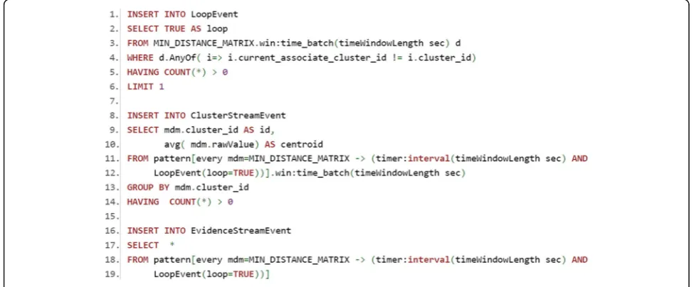
4.3 Online CEP-based K-means algorithm
An overview of the K-means algorithm work flow for on-line driving behavior detection is shown in Fig. 11. Unlike the previous modeling approaches, this is an iterative algo-rithm. Therefore, it is necessary to use a batch window to make iterating possible until the algorithm converges. Thus, the incoming evidence data stream is first separated in different temporal contexts (batch windows). Second, cluster centroids are chosen. The traditional implementa-tion of the K-means algorithm chooses K random in-stances and defines them as clusters’centroids. The main disadvantage of this method lies in its sensitivity to initial values of the cluster centroids. Our developing tests displayed a poor performance with the traditional random choice of initial centroid’s values of the clusters. To over-come this problem, the algorithm starts with previously acquired knowledge in the training phase. More details are given in Section 3.5.
Third, the distances between evidence and clusters centroids are calculated and evidence are assigned to the nearest cluster, as shown in Fig. 12. While some evi-dence changes from one cluster to another (Fig. 13 from line 1 to 6), the algorithm performs two parallel process-ing only if there is amin_distance_matrixevent followed byloopEvent equal to true in a specific time window: (i) new cluster centroids are calculated (Fig. 13, line 8–14) and (ii) the evidence is put back into the flow for an-other calculation of the distances to the cluster centroids (Fig. 13, line 16–19). Otherwise, the clusters are for-warded for driver behavior analysis. At the end of each batch window, if for most of the time the evidence be-longs to the cautious cluster, then the driver is classified as cautious. In any other way, the driver is classified as reckless. Thus, if a driver maintains a driving behavior Fig. 16Speed Z-distribution comparison
without abrupt changes of speed or direction, for in-stance, the percentage of evidences that belong to the cautious cluster is higher than to reckless cluster and the driver is classified as cautious.
4.4 Limitations
While CEP provides several benefits for data stream processing, such as continuous query, pattern detec-tion, and temporal windows, it is difficult to express iterative controls, e.g., while and for repetition struc-tures, using its primitives. Typically, CEP-based appli-cations follow a pipeline stage topology, with data flow in a given direction from one stage to one or more stages, but without returning to previous stages. This can be troublesome when describing iterative al-gorithms, such as K-means, which require iterations to converge. To overcome this problem, we simulated the loop check by using two EPL rules. If the loop check is false, i.e., if evidence has not change its cen-troid, we push the event to the next processing stages. However, if the loop check is true, i.e., evi-dence has changed its centroid, we reinsert these events into the initial loop stage, which recomputes
the centroid distance. We do so by translating the events to EvidenceStreamEvents, the event type that the initial loop phase (distance computation) expects.
Although useful, the independency of each CEP processing stage can difficult to coordinate between them. For instance, the proposed K-means algorithm buffers the received evidence in batches of Δ time period which are sent to the next processing stage, as shown in Fig. 12. This is required so that during in-teractions, the algorithm analyzes the same set of evi-dences to partition them into clusters. Thus, even though the events are buffered, the batch events are analyzed one by one by default in the sequential pro-cessing stages. To do so, the stages buffer the incom-ing events in a minimum window so they can be output as a batch. This minimum time window is associated with the mobile device memory and pro-cessing power and is usually less than a second. This limitation is shown in the EPL rule at the top of Fig. 13. The timeWindowLength parameter is the minimum time for to buffer all outputted streams in the min_disntance_matrix event and check if evidence has changed its centroid.
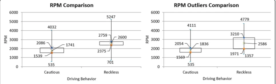
Fig. 18Speed comparison
5 Defining and planning the case study
In this section, the case study is presented with a focus on the definition and planning of the objective.
5.1 Objectives and contributions
The aim of this case study is to evaluate the designed and implemented algorithms, as shown in Section 4, to identify drivers’driving behavior based on outlier detec-tion. More specifically, the objectives are as follows.
- Evaluate the effectiveness of online outlier detection algorithms. That is, evaluate the performance analysis of the pattern recognition algorithms for online outlier detection in the context of limited computational resources (i.e., with a smartphone).
- Perform a case study to assess a driver’s driving behavior on driveway sections, such as roundabout, turns, tangent sections, semaphores, intersections (all-way stop), and crosswalks based on online outlier detection.
- Provide an open dataset of driver behavior with a rich set of sensed data, such as speed, rpm, throttle position, accelerometer, and gyroscope.
5.2 Research questions
The research questions that need to be answered through the case study are:
Which is the best algorithm in terms of accuracy?
Which is the best algorithm in terms of precision?
Which is the best algorithm in terms of recall?
Which is the best algorithm in terms of F-measure?
Which is the best algorithm in terms of average
execution time?
Which is the best algorithm in terms of resource
consumption (memory and CPU)?
5.3 Drivers and route selection
Due to the difficulty of recruiting drivers and the costs associated with assessing driving behavior, the process of driver selection was a matter of convenience and sam-pling was completed by quota. However, we attempted to establish a sample that represented a broad swath of drivers, preserving the same behavioral characteristics. Thus, 25 drivers were chosen for the study. Sixteen were male and nine female, their ages ranged from 20 to 60 years. Another important factor is driver experience. In our sample, driver experience ranged from 2 to 42 years. Finally, all drivers were familiar with local traf-fic condition and regulations. This is important so that during the assessment their behaviors reflect the daily driving habits.
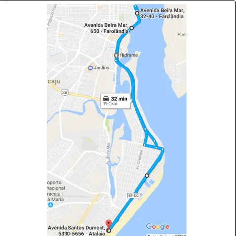
Regarding route selection, several potential test loca-tions were evaluated. We chose a paved route comprised of streets and avenues ranging from one to three lanes covering approximately 19.4 km in Aracaju-SE Brazil. In addition, the route, shown in Fig. 14, contains traffic lights, pedestrian crossings, and turns (including 45° and 90° turns). The speed limit on the route was 60 km/h. A pilot study was conducted with all the 25 drivers on the chosen route and this pilot study provided insight into drivers’behaviors.
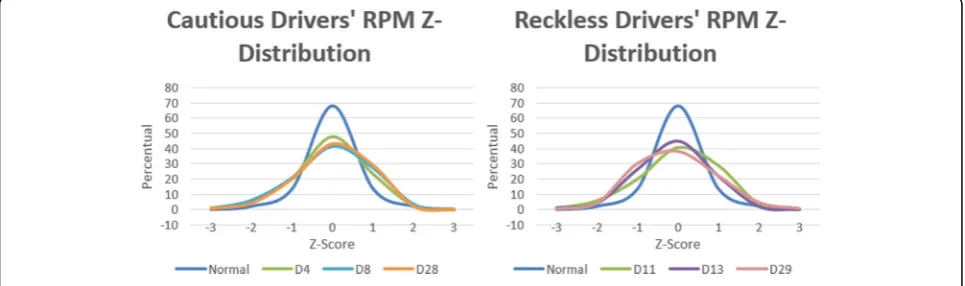
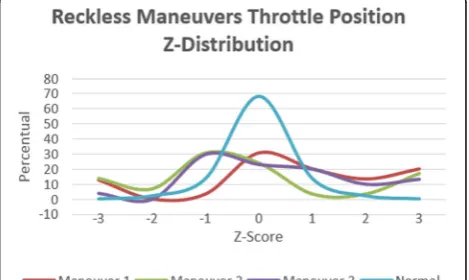
Fig. 20RPM maneuvers Z-distribution comparison
5.4 Instrumentation
The instrumentation process began with the implementa-tion of the algorithms through CEP rules as described in Section 4. The algorithms were implemented in EPL, an structured query like language (SQL-like) where streams replace tables as the source of data with events replacing rows as the basic unit of data for running in ASPER, a CEP processing engine based on ESPER (an open source CEP engine [81]) and adapted for Android.
A Brazilian version of the Citröen C3 manual trans-mission was equipped with a Samsung Galaxy SIII 1.4 GHz Quad Core with 1GB of RAM and a Bluetooth OBD-II device. Our prototype was installed in the smartphone running the online Z-score algorithm. Fur-ther details regarding the choice of algorithm are given in Section 6.4. The data collected by the prototype and processed by the Z-score were stored in SQLite [82], an embedded and free SQL database engine.
5.5 Measurement metrics
A confusion matrix is a suitable technique to evaluate the predictive ability of an algorithm to classify data in-stances, [83]. Fornclasses, the confusion matrix is table of n x n. The actual class column corresponds to the correct classifications and the predicted classrepresents the algorithms’classifications. When there are only two classes, one is considered positive (in our case, cautious driving) and the other is considered negative (reckless driving) [83], as shown in Table 1.
Thus, TP means that an instance of positive class is correctly classified as positive (cautious driving evi-dence), FN means that a positive class instance is mis-classified as negative (reckless driving evidence), TN means that a negative class instance is classified cor-rectly as negative, and FP means that a negative class in-stance is misclassified as positive. Based on a confusion matrix, we can calculate five performance metrics, shown in Table 2, which can be used to evaluate the al-gorithms. In addition, as a quality metric, we used the
average execution time, that is, the arithmetic mean of execution times for a given algorithm and the algo-rithms’average resources consumption.
6 Operation of the case study
This section describes the preparation and execution of the real world case study.
6.1 Preparation
To train the algorithms, we used the open dataset pro-vided by Bergasa et al. [57]. The dataset provides three axis accelerometer data labeled as cautious and reckless based on thresholds given by Paefgen et al. [54] for ac-celeration, braking, and turning. This dataset contains driving data for six different drivers and vehicles, D1 through D6, for two different routes, one is 25 km in a road with 3 lanes in each direction and a speed limit of 120 km/h, the other is ~16 km on a secondary road with one lane on each direction and a 90 km/h speed limit. Each driver drove the same route three times. For each driver’s data, a 3-fold cross-validation was performed, where each driver’s data are randomly divided into two pieces, one piece of 35% for training, and one piece of 30% for testing, and subset of data that generated the Fig. 22Throttle position Z-distribution comparison
best results for each algorithm checked. The training and testing hardware was the smartphone discussed in Section 5.4.
Regarding the K-means performance problem highlighted in Section 3.3, we randomly chose a driver and extracted driving data from cautious and reckless behavior from the training dataset and computed the clusters’centroids. Thus, the algorithm begins with previously acquired knowledge instead of choosing random values for the clusters’ cen-troids. With this strategy, the K-means algorithm signifi-cantly improved results, as is seen in Section 6.1.1.
To be operational on a mobile device, the applications need to vary the data rate based on the available compu-tation resources. So, the algorithms need to adapt their behavior to perform outlier detection with good accur-acy. Based on this scenario, we defined two setups. Firstly, we set the sensor data sample rate to be
h = 100 Hz and a time window of Δ = 10 s (setup 1). Second, we set the sensor data sample rate to be
h= 50 Hz and a time windowΔ= 20 s (setup 2).
6.1.1 Intrinsic evaluation of the knowledge model
In this subsection, we present the results of the training using the open dataset cited in Section 6.1. We repeated
each evaluation 5 times and the confidence level for all results is 95%. As shown in Table 3 and 4, the dataset contains more positive instances than negative instances. This data corroborates our first assumption, highlighted in Section 1.3. From the confusion matrix, we calculated the performance metrics defined in Table 2 for the two defined setups. The three algorithms had excellent per-formance, as the worst result classified 93.71% of evi-dences correctly and there is no significant (greater than 1%) difference between the average results, as shown in Table 5. Despite the good overall performance, the Z-score and K-means algorithms stood out with the high-est average accuracies.
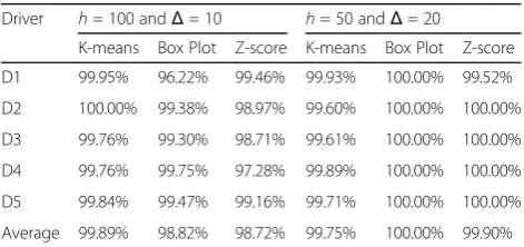
In the first setup, the box plot and Z-score had prac-tically the same precision and K-means had an impres-sive result with an average precision of 99.89%. This means that K-means correctly classifies 99.89% of cau-tious evidences. On the other hand, in the second setup, the box plot correctly classified all cautious evidences. Only K-means had worse precision, as shown in Table 6. According Table 7, the Z-score achieved a better recall performance in both setups. This means that, on aver-age, the Z-score reached better true positive rates. The K-means algorithm also achieved excellent results. Fig. 24Throttle position comparison
Regarding F measure, K-means and Z-score once more obtained similar overall performances and the box plot obtained a slightly lower performance in the first setup. However, in the second setup, the Z-score stood out with the highest average F measure, as shown in Table 8. Table 9 shows the execution time in milliseconds for each algorithm. It is possible to note that the Z-score re-quires considerably less processing time than the other algorithms and because the K-means requires computa-tion of pairwise distances for all evidences against cluster centroids, it has quadratic complexity, in contrast to the linear complexity of the box plot and Z-score. This ex-plains the large execution time. Furthermore, while the box plot and Z-score execute a single pass over the en-tire data stream, K-means requires, on average, three it-erations for each time window. The results confirm our intuition. For the chosen setups, there are no significant (greater than 1%) differences in each algorithm’s execu-tion time.
To check the algorithms’ resources consumption in both setups, we first verified the smartphone’s memory and CPU usage in two situations: standby and collecting data from the smartphone’s own sensors and OBD-II de-vice without processing them. It is possible to note in
Table 10 that merely collecting data increases memory consumption by 12.54% and CPU usage by 60.83%. By analyzing data from Table 11, it becomes clear that the Z-score outperforms the K-means and box plot algo-rithms in both setups, and K-means stands out nega-tively in terms of CPU usage. Moreover, a larger time window results in higher memory consumption and processing.
After reviewing these results and calculating the aver-age error rate of the algorithms, K-means and Z-score stand out with the lowest average error rates. Both had similar average rates, while the K-means achieved a bet-ter performance in setup 1 and the Z-score achieved a better performance in setup 2. Thus, regarding perform-ance metrics, K-means and Z-score obtained similar re-sults (difference between 0.1 and 1.1%). However, K-means obtained better results in setup 1 and Z-score in setup 2. The only exception was in the recall metric that the Z-score obtains the best result in both setups. Re-garding the quality metrics, the Z-score average execu-tion time was roughly seven times smaller than the K-means and two times smaller than the box plot. In addition, the Z-score required an average of 14% less memory consumption than the K-means and 8% less than the box plot. Finally, the Z-score required, on aver-age, a CPU usage of 68% less than K-means and 38.5% less than the box plot(Table12).
6.2 Comparison with the state of the art
To compare the approach used in this paper to classify driving behavior and therefore show its benefits, three related work were implemented. A simplified version of VEDAS [74] was developed, however, the piecewise lin-ear approximation algorithm was implemented based on the information provided by Keogh et al. [75] through CEP rules using sliding windows. The work of Aljaafreh, Alshabatat, and Najim [76] that uses fuzzy logic infer-ence for online identification of abnormal driving data was implemented using Fuzzylite [84], a free and open Fig. 26G-force maneuvers’Z-distribution comparison
source fuzzy logic control engine for multiple platforms, including Android. The Quintero, Lopez, and Cuervo [14] proposal was implemented. However, unlike the ini-tial proposal whose processing of fuzzy system variables is done offline by a neural network on a remote server, all processing was done on the smartphone using Neu-roph [85]. Nevertheless, we used the same configuration proposed by Quintero, Lopez, and Cuervo [14]–a two-layer neural network, with nine neurons in the inter-mediate layer, 31 inputs, and trained with a backpropa-gation algorithm. The Join Driving scoring mechanism was implemented according to Zhao et al. [55]. Finally, a machine learning model (naïve Bayes classifier) [56] using data from smartphone and OBD-II device was im-plemented. The performance evaluation process of each approach followed the steps described in section 6.1.
Table 13 shows the algorithms’ performance metrics. For the K-means, box plot, Z-score and piecewise linear approximation (VEDAS) implemented by CEP rules, Table 13 shows the average obtained in configurations 1 and 2. Through comparison of the results, it can be seen that the approach using neural networks resulted in a
superior performance in all the evaluated metrics except precision. In addition, the neural network obtained an extremely low error rate. However, the Z-score per-formed close to the neural network since, in percentage terms, for each metric the difference was always less than or equal to 1%. Join Driving [55] had a good per-formance, however, it scored below the previous ap-proaches. The Naïve Bayes classifier approach as presented by Hong, Margines, and Dey [56], clearly underperformed compared to the other approaches. It is worth mentioning that this result is compatible with the work of [86–88] in which a Naïve Bayes classifier did not obtain good results.
Comparing the quality metrics shown in Table 14, it is notable that the Z-score memory consumption was 1.10%, 10.30%, 54.30%, 0.79%, and 50.11% more efficient than the VEDAS, fuzzy logic, back-propagation, Join Driving and Naïve Bayes classifier, respectively. Among the approaches that analyze a set of instances belonging to a time window to determine which are outliers, the Z-score undoubtedly obtained the best result. The fuzzy logic, neural network with backpropagation algorithm, Fig. 28Acceleration analysis
Join Driving and Naïve Bayes classifier approaches clas-sified an instance as an outlier or normal, respectively, in ~10, ~11, ~10.6 and ~15 milliseconds. However, con-sidering a sensor update rate of 100 Hz and a time win-dow of 20 s, there are 2000 instances to be analyzed. The Z-score takes ~100 milliseconds to analyze all these data and classify each instance as normal or an outlier. This is an average of 0.05 milliseconds per instance ana-lyzed. Through this reasoning, the Z-score takes less time to process an instance. Regarding CPU usage, the box plot and Z-score achieved the best performances. However, the Z-score consumed 73.32%, 73.60%, and 74.13% less CPU than VEDAS, fuzzy logic, and backpro-pagation, respectively.
6.3 Execution
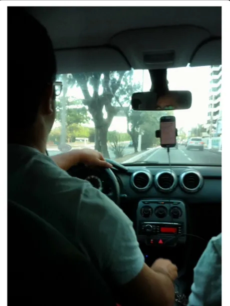
The smartphone was installed in the center of the ve-hicle windshield, as shown in Fig. 15. The OBD-II reader device was connected to the OBD-II port of the vehicle and read a variety of data from the vehicle bus. The OBD-II device sent the data streams via Bluetooth to the smartphone. Execution of the case study consisted of performing the process of outlier detection on driving data streams for each volunteer driver.
6.3.1 Data collection
Driver behavior data were collected over seven sunny days and the volunteers drove between 9 AM and 8 PM. Each driver made one trip on the chosen route. Thus, a total of 485 km was covered, comprising 20 h of driving. In addition, before the execution of the case study, the purpose of the study and the absolute confidentiality of personal information was explained to each volunteer.
Then, the chosen route was explained in detail and drivers were asked to drive as they usually would. The vol-unteer driver was also informed that a driving expert with 15 years’ experience would follow him or her during the case study—similar to an expert-based test administered in initial tests to judge driver performance—but we em-phasized that our goal was to analyze and classify the driver’s behavior as cautious or reckless, and not to ap-prove or disapap-prove of the actions. This classification served as a ground truth.
The prototype collected data from smartphone sen-sors (i.e., accelerometer, gyroscope, magnetic compass, and GPS) and vehicle sensors (i.e., speed, RPM, and throttle position percentage) through the OBD-II de-vice. These sensors’ data streams were sent to the smartphone via the Bluetooth connection. The con-nection between the smartphone and OBD-II device was facilitated using generic mobile middleware [79] for short-range communication.
6.4 Extrinsic evaluation of the knowledge model
According to Bramer [83], there is no infallible way of finding the best classifier for a given application. None-theless, regarding the quality metrics of CEP-based on-line outlier detection algorithms, the Z-score obtained an undoubtedly better performance; regarding perform-ance metrics, the Z-score and K-means achieved similar performances, as shown in Section 6.1.1. Thus, for this reason, the online Z-score algorithm was used to analyze
Fig. 30Normal scores probability
Table 15Online Z-score performance
Metric Value
Accuracy 95.45%
Recall 92.86%
Precision 100.00%
F-Measure 96.30%
Error Rate 4.55%
RAM(MB) 6.35 MB