VADA: an architecture for end user informed
data preparation
Nikolaos Konstantinou
1, Edward Abel
1, Luigi Bellomarini
2, Alex Bogatu
1, Cristina Civili
3, Endri Irfanie
1,
Martin Koehler
1, Lacramioara Mazilu
1, Emanuel Sallinger
4, Alvaro A. A. Fernandes
1, Georg Gottlob
4,
John A. Keane
1and Norman W. Paton
1*Introduction
As a result of emerging technological advances that allow capturing, sharing and stor-ing of data at scale, the number and diversity of data sets available to organisations are growing rapidly. This is reflected, for example, in the adoption of data lakes, for which the market is predicted to grow at 28% per year from 2017 to 2023 to $14B.1 This data creates unprecedented opportunities, but only if the deluge of data can be turned into valuable insights.
Abstract
Background: Data scientists spend considerable amounts of time preparing data for analysis. Data preparation is labour intensive because the data scientist typically takes fine grained control over each aspect of each step in the process, motivating the devel-opment of techniques that seek to reduce this burden.
Results: This paper presents an architecture in which the data scientist need only describe the intended outcome of the data preparation process, leaving the software to determine how best to bring about the outcome. Key wrangling decisions on matching, mapping generation, mapping selection, format transformation and data repair are taken by the system, and the user need only provide: (i) the schema of the data target; (ii) partial representative instance data aligned with the target; (iii) criteria to be prioritised when populating the target; and (iv) feedback on candidate results. To support this, the proposed architecture dynamically orchestrates a collection of loosely coupled wrangling components, in which the orchestration is declaratively specified and includes self-tuning of component parameters.
Conclusion: This paper describes a data preparation architecture that has been designed to reduce the cost of data preparation through the provision of a central role for automation. An empirical evaluation with deep web and open government data investigates the quality and suitability of the wrangling result, the cost-effectiveness of the approach, the impact of self-tuning, and scalability with respect to the numbers of sources.
Keywords: Data preparation, Data quality, Data integration
Open Access
© The Author(s) 2019. This article is distributed under the terms of the Creative Commons Attribution 4.0 International License (http://creat iveco mmons .org/licen ses/by/4.0/), which permits unrestricted use, distribution, and reproduction in any medium, provided you give appropriate credit to the original author(s) and the source, provide a link to the Creative Commons license, and indicate if changes were made.
RESEARCH
*Correspondence:
1 School of Computer Science,
University of Manchester, Oxford Road, Manchester, UK Full list of author information is available at the end of the article
However, extracting value from such data presents significant challenges, not only for analysis, but also when preparing the data for analysis. Obtaining a dataset that is fit for purpose is expensive, as data scientists must spend time on the process of data prepa-ration, also referred to as data wrangling, which involves identifying, reorganising and cleaning data. It is reported that data scientists typically spend 80% of their time on such tasks.2 In relation to the V’s of big data Volume, Velocity, Veracity, Variety and Value, this paper proposes techniques that enable Value to be obtained from data sets that exhibit
Variety in terms of how data is represented, and manifest Veracity problems in terms of consistency and completeness. We also show how Volume can be addressed by present-ing experiments that involve significant numbers of sources, and accommodate Velic-ity in terms of rapidly changing sources by automating the creation of data preparation tasks.
Several data preparation approaches are in widespread use; in practice data prepara-tion tends to involve either programming the soluprepara-tion (e.g., [1]), developing extract– transform–load workflows (e.g., [2]) or developing transformations over a tabular representation of the data (e.g., [3]). Data preparation tools tend to provide components that support similar tasks (e.g., joining data sets, reformatting columns), but differ in how these are expressed by data scientists. However, even with tool support, the prin-cipal development model is that a data scientist retains fine-grained control over the specification of a data preparation task. There are clearly circumstances in which this is appropriate, but the associated costs are high and sometimes prohibitive, motivating the investigation of more automated approaches.
Contributions
In this paper, we present the VADA (Value Added Data Systems) architecture that puts automation at the core of an end-to-end data preparation system. To automate data preparation, several challenges must be addressed, including: (i) the orchestration of a diversity of data preparation components that depend on different evidence about the problem to be solved; (ii) the accommodation of different components for the same task, and alternative approaches; (iii) the identification of evidence that can inform several of these steps, so that, e.g., the provision of training data is not burdensome; (iv) the selec-tion between alternative candidate soluselec-tions, in the light of multiple, potentially con-flicting, requirements; (v) the configuration the parameters of multiple inter-dependent components; and (vi) the revision of solutions in the light of feedback.
We show how a data product can be obtained from a large number of sources, without the need to hand craft processing or transformation rules or scripts. We focus on the challenges in designing an automated, end-to-end, dynamic, cost-effective data prepara-tion system architecture, and on the integraprepara-tion and evaluaprepara-tion of the system as a whole. The research contributions are as follows:
a. An architecture in which loosely coupled data preparation components are declara-tively and dynamically orchestrated, allowing different components to run depending on the available information, and supporting self-tuning of configuration parameters.
b. An approach to automating data preparation that takes into account user preferences and user feedback; the preferences deploy techniques from multi-criteria decision analysis to trade-off (potentially) conflicting data quality criteria, and the feedback allows the system to revise wrangling decisions.
c. An evaluation of the resulting approach in terms of the quality (precision) and suit-ability (with respect to user criteria) of the result, the impact of feedback, the cost savings compared with manual data wrangling, the runtime of the wrangling process, and the impact of self-tuning for inter-dependent components.
Motivating example
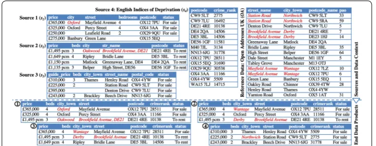
Consider a data scientist with the task of getting insight from several datasets in the real estate domain. To do so, data is extracted from a collection of real estate sites, using web scraping or specialised data extraction software. In Fig. 1, above the dotted line, is the data provided as input to the wrangling process, specifically: Source 1 to 3—fragments of real estate data automatically extracted from web data sources; Source 4—open govern-ment data containing the UK indices of deprivation; and Reference data—a list of street names, cities/towns and postcodes in the UK. At the bottom of the figure, are results of the following four data preparation scenarios obtained with VADA.
Scenario 1: Basic case
We obtain an end data product in a fully automated manner. In this scenario, the user provides only the set of sources (Sources 1 to 4), the schema of the end data product (price, city_town, beds, street, postcode, crimerank, status), and a targeted size for the end data product (3 tuples). The system infers properties of the sources using data pro-filing, carries out matching and mapping generation to populate the end product, and prioritises the selection of complete tuples for the result. The result is end data product ➀ below the dotted line in Fig. 1.
Scenario 2: Data Context
Data context is instance data aligned with the target that is used to inform the behav-ior of several wrangling components. Note that the sources to be wrangled are typ-ically disjoint from the data sets participating in the data context. In this example, the data context consists of reference data with street_name, city_town and postcode
(top right of Fig. 1) aligned with the corresponding attributes in the target. The sys-tem is now able to synthesise and apply format transformation rules on attribute val-ues, based on the data context. Using these, it will transform the incorrect values in
s2.str_name , e.g. from the incorrect Brookfield Avenue, DE21 to the correct
Brookfield Avenue. Moreover, the system is also able to mine rules in the form of conditional functional dependencies (CFDs) from the data context (following the approach of [4]), which can be used to repair the initial end product [4]. For example, the following CFDs are learnt from the reference data:
property([street_name] → [city_town], (Mayfield Avenue || Wantage)) property([street_name] → [city_town], (Brookfield Avenue || Derby)) property([street_name] → [city_town], (Station Road || Northwich))
By using these rules to repair the end product, the incorrect values Oxford and Oakwood in end data product ➀ are now replaced with the correct ones, Wantage and Derby, respectively. The transformed and repaired result is end data product ➁ in Fig. 1.
Scenario 3: User context
The user context captures user preferences using criteria relating to data quality. Even though end product ➁ is now consistent w.r.t. the data context, it may not be fit for purpose because users have different needs. A user may decide that they are interested in properties whose street name appears in the data context, and with a known number of bedrooms. In this case, the user states in the User Context that completeness wrt. the data context in attribute street and completeness of the values in attribute beds are important. This informs the system that these tuples are preferable. The result of the process is data product ➂ in Fig. 1.
Scenario 4: Feedback
Feedback takes the form of annotations from the user on an end data product. In this example, the user indicates in end data product ➂ that the status value To rent and the beds value 4 are not relevant. After these feedback instances have been taken into account, the system will prefer data sources that reflect this feedback, and the result is end data product ➃ in Fig. 1.
Methods
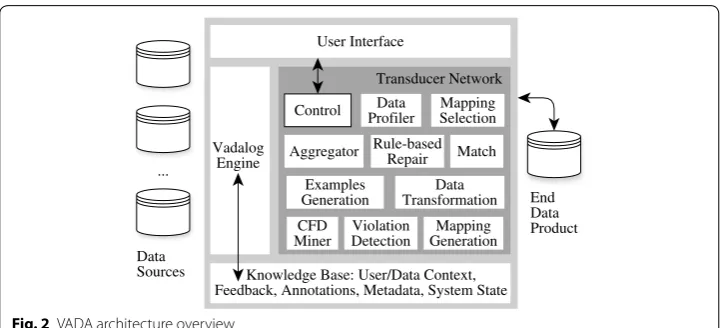
Architecture overview
This section describes key features of the architecture, illustrated in Fig. 2. In the User Interface, the target schema is defined, and provided with associated instance evidence in the Data Context and priorities of the user in the User Context. In the light of this information, the system orchestrates a collection of data wrangling components, to pop-ulate the End Data Product from the Data Sources. The user can then provide feedback on the End Data Product, which is taken into account in the production of a revised result. The individual wrangling components are represented using relational transduc-ers [5], and they are declaratively orchestrated using the Vadalog Engine [6]. The Vadalog Engine is centered around Vadalog, a reasoning language whose core is Warded Data-log± , and augments Datalog programs (sets of function-free Horn clauses) with exis-tentials, as well as with stratified negation, but introduces syntactical restrictions to guarantee tractability of reasoning tasks. The Knowledge Base holds information about the data wrangling scenario. As such, its contents include: (a) metadata about sources and data products such as URIs, relation names, attribute names, and basic statistics; (b) metadata about the target schema; (c) metadata about the workflow such as current state and provenance information; and (d) User Context, Data Context and feedback.
We now relate Fig. 2 to each of the scenarios from the Motivating Example. In Scenario 1, as the user has provided only the sources and the target, there is no data context. As a result, with a basic Control transducer, only the Match, Data Profiler, Mapping Gen-eration and Mapping Selection transducers are run to produce the End Data Product. In
Scenario 2, data context is now also available in the knowledge base, providing additional evidence to inform data preparation, enabling the Examples Generation, Data Transfor-mation, CFD Miner, Violation Detection and Rule-based Repair transducers to be evalu-ated in addition to the transducers used with Scenario 1, to produce an improved End Data Product. In Scenario 3, as user context has been provided, the Mapping Selection
transducer applies the given criteria to identify how mappings should contribute to the
End Data Product. In Scenario 4, as feedback is now also available to inform the user context, Mapping Selection is run again, selecting different tuples from the mappings, in the light of the additional evidence from the feedback. The remainder of this section details cross-cutting features of the architecture.
User Interface Match Mapping Generation CFD Miner Rule-based Repair Data Transformation Examples Generation Violation Detection Mapping Selection Data Profiler Control Transducer Network Vadalog Engine
Knowledge Base: User/Data Context, Feedback, Annotations, Metadata, System State
Aggregator Data Sources ... End Data Product
User interface
Rather than taking fine-grained control over how wrangling is to take place, the user provides information about what is required from the wrangling process.
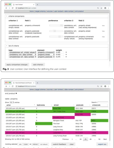
As illustrated in Figs. 3 and 4, the web interface provides the following tabs: Home:
supports the management and execution of data wrangling activities. Target schema: supports the specification and revision of the schema that is to be populated. Sources:
identifies the sources from which instance data is to be obtained for populating the tar-get. User context: enables the specification of user preferences, in the form of weights for different criteria, where these weights are derived from pairwise comparisons among the
Fig. 3 User context. User interface for defining the user context
criteria. Pairwise comparisons have been successfully deployed for multi-criteria deci-sion support [7], and have been shown to be promising in a usability study relating to data set selection [8]. In Fig. 3, a slider is used to indicate that the consistency of the street
has very strong importance compared with the completeness of the crimerank. Data con-text: enables the user to associate data sets from the domain with columns in the target schema. Such data sets act as evidence for different wrangling components. End product:
enables the user to browse, export and provide feedback on the end data product. For example, in Fig. 4 the user is indicating which result tuples or values in these tuples are
relevant.
As a result, the user interface principally provides access to the knowledge base from Fig. 2, providing data and metadata that are used by the components of the architecture to wrangle the data from the sources into the end data product. Note that the configura-tion of the wrangling task through the interface, for example through the provision of the data context data, is a one-off fixed cost. There is no need for the user to manually interact with or transform data sources, the variable cost that dominates manual data preparation. The web interface has been demonstrated at an earlier database conference, and is described in more detail by Konstantinou et al. [9].
Transducers
The data wrangling functionality, for example for mapping generation or format trans-formation, is implemented as a collection of loosely coupled components that build on the concept of a relational transducer (or simply transducer). Transducers were intro-duced by Abiteboul et al. [5], and have been successfully applied and extended in a vari-ety of applications [10], including web data extraction [11].
Transducers A transducer schema S is a tuple (in, out, state, log, db) of relational schemas for input, output, state, log and external database [5]. We extend S by a set of
parameter names that transducers can be parameterised by. The log maintains informa-tion about the input-output exchange, enabling the recording of system-level data lin-eage. A transducer class over schema S is a tuple TC=(δstate,δout,δguard,δscopes,δmap) where:
• δstate (resp. δout ) [5] are Vadalog rules or Java programs that describe the state transi-tion (resp. output) functransi-tion.
• δguard [11] are Vadalog rules that describe whether a transducer is ready to be exe-cuted.
• δscopes [11] are Vadalog rules that describe the scope of the transducer (i.e., parts of the knowledge base and external sources that the transducers depend on).
• δmap are Vadalog rules that describe the mapping between the knowledge base and other external schemata, and the internal schema of the transducer.
A transducer configuration CF for transducer class TC is a set of key-value pairs,
CF = {(K1,V1),. . . (Km,Vn)} where each Ki is a parameter name in S. A transducer instance is a transducer class together with its configuration.
declaratively; we have used this feature to plug in different wrangling components and implementations, with few or no changes required to other transducers or the user interface.
Transducer orchestration
While any programming language could be used to implement the data processing pipe-line, the use of transducers enables a high-level, declarative specification of the work-flow, without the need to explicitly specify its step sequence.
In VADA, transducer networks [12] are deployed to dynamically orchestrate the work-flow. Intuitively, a transducer network is a set of transducers, with a distinguished control transducer whose output determines the control flow of the transducer network. A con-trol transducer is responsible for orchestrating the transducers that directly process the data. Transducer networks can be arbitrarily nested, creating transducer subnetworks.
Transducer network Based on the notation introduced in [12], a transducer network
(which we shall also call a workflow specification) N is a tuple (Ctl, T, S), where:
• Ctl is the control transducer, a transducer determining control flow and dependen-cies in the transducer network.
• T is a set of transducer instances.
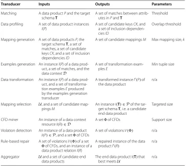
Table 1 Transducer inputs, outputs, and configuration parameters
Transducer Inputs Outputs Parameters
Matching A data product P and the target schema T
A set of matches between attrib-utes in P and T
Threshold Data profiling A set of data product instances
I(P) A set of candidate keys
CK, and a set of inclusion dependen-cies ID
Overlap threshold
Mapping generation A set of data products P, the target schema T , a set of matches, a set of candidate keys CK, and a set of inclusion dependencies ID
A set of candidate mappings M Max mapping size, k
Examples generation An instance I(P) of a data prod-uct, a set of matches, and the data context D
A set of transformation
exam-ples E Min tuple size
Data transformation An instance I(P) of a data prod-uct, and a set of transforma-tion examples E produced by the examples generation transducer
A transformed instance I′(P) of
the data product n/a
Mapping selection U , and a set of candidate
map-pings M An instance I
(T)∈P of the
tar-get schema T , i.e. a candidate
end data product
Targeted size
CFD miner An instance of a data context resource I(R)∈D
A set of CFDs Support size Violation detection An instance of a data product
I(P)∈P , and a set of CFDs
A set of violations V(�) n/a Rule-based repair A set of violations V(�) of a set
of CFDs, and an instance of a data product relation I(R)
A repaired instance of the data product I′(R) n/a
Aggregator U and a set of candidate end
data products The end data product I
(T) that best meets U
• S is a set of transducer subnetworks. A transducer subnetwork is defined recur-sively, i.e., is a transducer network itself.
Workflows are instances of a workflow specification. Execution of a workflow leads to the creation of a candidate end data product. Workflows are orchestrated by network transducers without user intervention, and they are responsive, in the sense that the system is able to monitor changes in the available data in the system and respond to opportunities as they arise to use information and revisit conclusions and the behav-iour of components in light of new information. Workflows are also dynamic, in the sense that the order of orchestration depends on the results of previous component runs. As such, automated wrangling stems from the dynamic orchestration of the loosely coupled data preparation transducers.
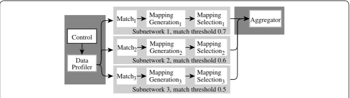
Figure 5 illustrates a simple scenario where transducer subnetworks explore alter-native configurations, and the Aggregator, as described in Table 1, selects the one that leads to the most suitable candidate data product. The three subnetworks in Fig. 5 test the match threshold, but other properties of other transducers could be tested as well in parallel, giving a form of self-tuning.
Listing 1 is the Vadalog code that expresses the logic of the control transducer in Fig. 5, simplified for the sake of clarity. The @network annotation in line 1 informs the Vadalog engine that this is a control transducer. Then, two transducer instances and three subnetworks are defined (lines 2–3, and 4–6, respectively). The guard rules
δguard (lines 7–11) indicate when the transducer instances are ready to be executed,
based on the current state of the network expressed in executed. The core logic of this simple program, δout , is captured next (lines 12 and 13), stating that the next
transducer or transducer network to be executed is one whose input dependencies are satisfied, and that is not already executed. Note that, as part of the actual exe-cution of the transducer, once the transducer or network selected by nextTr (resp. nextSubnet) has actually been executed, the executed relation will be updated with that fact. Control transducers can also be defined for subnetworks, such as those illustrated in Fig. 5, providing flexible orchestration for tasks such as the exploration of alternative parameter settings.
Control transducer execution terminates after all transducers and transducer net-works have been executed. Vadalog has declarative semantics, therefore the order of the statements in Listing 1 is not significant.
Match1 Mapping Generation1
Control Subnetwork 1, match threshold 0.7 Match2
Mapping Generation3
Subnetwork 2, match threshold 0.6
Match3
Mapping Generation2
Subnetwork 3, match threshold 0.5
Aggregator Mapping
Selection1
Mapping Selection2
Mapping Selection3
transducer subnetwork transducer instance Data
Profiler
transducer network
Provenance Provenance information is used to inform the user how the end data prod-uct has been obtained. It is recorded at two granularity levels: at workflow level (coarse-grained), and at data level (fine-grained) [13]. The log of the transducers is responsible for recording workflow provenance [5]; the system maintains an execution log in which every transducer execution is recorded, along with its configuration.
Provenance at data level is supported by an additional provenance attribute added to source data when it is processed by the transducers. In cases when information is inte-grated or fused from multiple sources, all contributing sources will be recorded. As a result, the system can track tuples in the end data product back to their sources of ori-gin. For instance, the provenance information for the tuples of end data product ➀ in Fig. 1 will include both sources that contributed to the creation of each tuple, namely s1 , s4 for tuples 1 and 2, and s2 , s4 for tuple 3.
Data wrangling in context
Data wrangling in VADA takes place in the context of data from the domain in which wrangling takes place (data context) and priorities provided by the user (user context). Here we introduce several concepts that are used to define data and user context more precisely in due course.
A Data Collection is a set R= {r1,. . .,rk} of relations from the knowledge base; these relations may represent data sources, or the results of data wrangling operations, such as those illustrated in Fig. 2. Each relation ri∈R has a schema si , that is a set of named, typed attributes. Attributes are written as r.a. The extent of a relation r (resp. attribute
r.a) is denoted by I(r) (resp. I(r.a)).
Data context Data context consists of data from the domain in which wrangling is taking place. Data context is used by several wrangling components to make better informed decisions. Although individual data integration components necessarily use evidence to support decision-making, the notion of data context cuts across individual components, so that one source of evidence is used in several places. Data Context D is
defined as pair (SDC,L) , where SDC is a set of Data Collections, and L is a set of data
con-text relationships. A Data Context Relationship is an association between a data context relation or attribute, and a data product relation or attribute. From the user’s perspec-tive, a data context relationship is defined on the target, but the system may propagate such relationships to other data products.
Two kinds of data context relationship are defined: at the entity level, Lent :R−→ent C , and at the attribute level, Latt :R.a−att→C.b , where R is a relation in a data context Data Collection SDC , and C is a relation from an intermediate or final data product.
Data context resources can be divided into subsets. For this paper, we consider the subsets E , M , and R of the resources available in SDC , where: E refers to example data
that could be found in the end data product, M to master data (i.e., a comprehensive and curated data set describing entities of interest to an organisation), and R to reference data (i.e., a complete collection of the values that the given attributes can legitimately hold).
In Fig. 1, the data context relationships for reference data OA are as follows:
Lent1 :OA−→ent T Latt1 :OA.street_name
att
−→T.street
Latt2 :OA.city_town att
−→T.city_town
Latt3 :OA.postcode_name att
−→T.postcode Lent2 :s1
ent
−→OA Latt4 :s1.city
att
−→OA.city_town Latt5 :s1.street
att
−→OA.street_name
Latt6 :s1.postcode att
−→OA.postcode_name
There are initially one entity-level relationship and 3 attribute-level relationships between the data context table OA and the target T, as shown in the first 4 relationships above. The further relationships are generated for source s1 after propagation.
User context Different applications, even over the same data may have different data quality priorities, and automated approaches to data preparation can generate many candidate data products. The user context allows the user to specify the characteristics of a data product that are most important. This information is then used to inform map-ping selection. Although others have developed criterion-based approaches to data set selection [14], user context is distinctive in deploying multi-criteria decision support with user-specified weights over diverse criteria.
The user context U consists of a set of criteria C and a function w:U → [0, 1] , such that
ci∈Cw(ci)=1 . Criteria are associated with either the target schema T , or an attribute T.a of T.3
Every criterion c∈C is of a specific criterion typecT , including, for instance,
com-pleteness, accuracy and relevance. Every criterion type is associated with an evaluation function f(cT,p) . Thus, a criterion c of type cT is evaluated by executing a criterion eval-uation function f(cT,p):U×P →A , that is a function that once evaluated on a data product p∈P for a criterion c∈U will produce an annotation from A , the set of all annotations. Annotations are tuples of the form (p, c, a) where p∈P is a data product,
c∈U is the evaluated criterion, and a is a numeric value with a∈ [0, 1] , that is the result
of the criterion evaluation.
The criteria that are available are domain-independent, though extensible, and fall into the following categories: standalone (such as completeness wrt. empty values, type match, or pattern match), data context-related (such as accuracy, completeness or con-sistency wrt. data context), or feedback-related being subjective to the user (such as use-fulness, relevance or correctness).
Criterion evaluation functions often compute the fraction of the values that satisfy a prop-erty. For example, for a data product attribute p.a associated by an attribute level data context relationship with data context attribute d.c, for the types of criteria in Fig. 3, we have:
• Completeness w.r.t. empty values, the fraction of the values in p.a that are not null: count({v|v←I(p.a),v<>null})
|I(p.a)| ;
• Consistency w.r.t. data context, the fraction of the values for p.a can be found in d.c: |I(p.a)∩I(d.c)|
|I(p.a)| ; and
• Completeness w.r.t. data context, the fraction of the values in d.c that can be found in p.a: |I(p.a)∩I(d.c)|
|I(d.c)| .
Data wrangling components
As previously discussed, components that take part in the data wrangling process are represented as transducers, and thus are orchestrated dynamically, for example when suitable inputs are available. In this section we zoom into their specifics. We note that all transducers are pluggable components, and that alternative implementations could be incorporated. We now describe in more detail the transducers in Table 1.
Matching and profiling
This section introduces the transducers that identify basic similarity relationships between data products.
Matching Given a data product P and target schema T , the transducer will identify candidate matches between every attribute in P and every attribute in T . Matches are tuples of the form (P.a,T.b,score) , where P.a is an attribute in P, T.b is an attribute in T and score is a similarity score, with score∈ [0, 1] . Where more than one attribute from a data product table matches a single attribute from the target table, the match with the higher score is retained.
for which this is possible are the ones that are associated with at least a data con-text relationship to the respective reference/master/example data. For this case, we have implemented an index-based matcher [16], which first tokenises all cell values in source and target attributes, and then builds an inverted index I∗ for each one of them. Tokens thus become inverted index keys. A stop-word list is used to filter out tokens of low importance (e.g., “and”, “the” or “a”).
To compare the similarity score between I(P.a) and I(T.b) , first we merge their
inverted indexes into an also inverted index I∗ . We then create two sets: VP.a are val-ues that appear in I(P.a), and VT.b values that appear in I(T.b) . The average similarity score is then calculated as:
i is an index entry in I∗ , |I∗| is the total number of index entries, ViP.a is the set of values in i that appear in VP.a , ViT.b is the set of values in i that appear in VT.b , and sim is the
Jaro similarity metric.
A second evidence of similarity, the inclusion score, is defined as the ratio of the number of distinct values |I∗| in the merged index I∗ over the number of distinct
val-ues from VP.a and VT.b . As such, inclusion score is defined as:
In the absence of attribute names, the overall similarity score between I(P.a) and I(T.b) is estimated as:
When attribute names are available, the maximum of the two similarity evidences is combined with the attribute name similarity attNameSim, to estimate the overall simi-larity score between I(P.a) and I(T.b) as:
Data profiling This transducer analyses the given set of data products, for which it pro-duces a set of candidate keys CK, and a set of (partial) inclusion dependencies ID of the form (g1,g2,overlap) , where g1 and g2 are groups of attributes of the data products,
and overlap the ratio of the values of the attributes in g1 included in the values of the attributes in g2 . If both overlaps ( g1 in g2 and g2 in g1 ) are below a configured overlap threshold, the inclusion dependency is discarded. Sets CK, ID (and matches) serve as inputs to the mapping generation transducer, where they underpin decisions as to which operators should be used in candidate mappings and on the fitness of candidate map-pings. The implementation builds on Metanome [17], using HyUCC for candidate key discovery [18] and Sindy [19] for detecting (partial) inclusion dependencies. In building on readily available profiling data, we enable downstream decisions to be made without the need to provide additional training data sets.
(1)
avgSim= 1 |I∗|
i∈I∗
sim(ViP.a,ViT.b)
(2)
incScore= |I ∗|
distinct(VP.a∪VT.b)
(3)
Score=
1
2(avgSim
2+incScore2)
(4)
Score=
1
2(attNameSim
Mappings
This section introduces the transducers that generate and select mappings that are used to populate the target from the sources.
Mapping generation This transducer, given matches between data sources and the tar-get and profiling information (candidate keys and partial or full inclusion dependencies) that describes source tables and relationships among them, generates a set of candidate mappings from source to target tables.
Mapping generation has at its core a dynamic programming method, through which a complex problem is divided into sub-problems that are easier to solve, which then are used to compose the solution for the complex problem. In our case, generating mappings for a set of sources represents the complex problem, and this is divided into simpler sub-problems where the algorithm finds mappings for subsets of the sources. During map-ping generation, the fitness of a mapmap-ping is based on an estimate of the number of largely complete tuples it will return, so the algorithm chooses the mappings that are likely to return more complete tuples than other mappings. In each iteration of the algorithm, the number of input relations of generated mappings (sub-solutions) is increased, until it reaches a configured max mapping size. Profiling data is consulted to decide on the most meaningful operator to apply when merging mappings, e.g. union when mappings have matches to the same target attributes or, if matches differ, join on candidate keys with a full inclusion dependency (overlap of 1.0), or full outer join on candidate keys with the highest overlap otherwise. Profiling data is propagated from base tables to candi-date mappings. The output of the transducer is a set of k candidate mappings (involving union, join, and outer join), ranked on their fitness.
For this scenario, a total of 9 mappings are generated, m1:s4⊲⊳s1 , m2:s4⊲⊳s2 , m3:s4⊲⊳s3 ,
m4:s1∪s2, , , , ,
and , joining on the postcode attributes. Mapping m2 is given in full in Listing 2. As such, in relation to schematic heterogeneities, mapping generation can address horizontal and vertical partitioning in sources.
Mapping selection This transducer selects tuples from the candidate mappings in order to populate a candidate end data product. The approach is based on the multi-criteria source selection proposal of Abel et al. [15], the role of which here is to popu-late a candidate end product that best meets the criteria in the user context using the data from the candidate mappings. The fitness of the candidate mappings is evaluated using the overall weighted utility (OU) function, introduced in [15], calculated as:
B is the targeted size, wj is the weight of criterion j, C is the number of criteria, qi is the number of tuples selected from the candidate mapping i, cij is the result of evaluating cri-terion j on the candidate mapping i, and Zj∗ (resp. Zj∗∗ ) is the ideal (resp. negative ideal)
solution for criterion j, i.e. the maximum (resp. minimum) value for this criterion, if this was the only criterion in the user context. The transducer tries to determine the tuple selection solution that best meets the user requirements, by optimising the OU for the resulting candidate end product.
The result of the mapping selection process is a vector of the quantity of tuples to be used from each mapping in populating the end product, with the sum of the quanti-ties being equal to the targeted size. In the example Scenario 1 of Fig. 1, 9 candidate mappings are available, m1,. . .,m9 , as previously detailed in the mapping generation
transducer, and the resulting quantity vector is {0, 0, 0, 0, 0, 3, 0, 0, 0} , thus leading to selection of 3 tuples from m6 to populate a candidate end data product.
Aggregator In self-tuning, when different configuration parameters are being inves-tigated, there may be several candidate end data products. In this case, the Aggrega-tor transducer selects among these candidates the one that is most fit for purpose. To evaluate their fitness, the Weighted Sum (WS) metric is used, defined as the evalua-tion of all criteria metrics multiplied by their respective weights:
wj is the weight of criterion j, and cj is the result of evaluating criterion j on the candidate
end data product. The Aggregator then selects the candidate with the maximum WS. Note that a difference between Eqs. 5 and 6 is that the former acts on candidate mapping properties (and is evaluated more often within the optimisation process), whereas the latter uses the results of the candidate end data products.
(5) OU = 1
B S
i C
j wjqi
cij−Z∗∗j Z∗
j −Zj∗∗
(6)
WS=
C
Format transformation
This section introduces the transducers that synthesise and apply data format transformations to attributes in data products; these can be applied either to indi-vidual sources or to the results of mappings. This transducer synthesises format transformation programs from examples, taking inspiration from prior work such as FlashFill [20].
Examples generation To automate the process of obtaining format transformation programs, this transducer focuses on automatic discovery of examples that can be used for synthesis. Building on the approach of Bogatu et al. [21], it discovers exam-ples by aligning values found in matching data product and data context attributes, and then minimises the initial set of candidate examples, creating a set of examples as illustrated below.
Examples automatically generated from attribute street_name in reference data; here the input →output examples relate input values in which the street name has been supplemented in a source with some additional information that is not present in the definitive street name, and made available in the data context.
Mount Terrace, Brampton Road → Brampton Road Plot 3 Coward Drive → Coward Drive
Cottage, Mountenoy Road → Mountenoy Road The Limes, 36 Broom Lane → Broom Lane
The minimum number of tuples for any candidate column pair to identify examples from is configured by min tuple size (set to 10 in all experiments in this paper). Larger values for min tuple size increase the time taken for transformation program synthesis, but also reduce the risk that relevant cases are overlooked during transformation synthesis. In the presence of profiling data, the transducer will not seek to generate examples for can-didate keys, as changing identifiers is likely to lead to undesired consequences.
Data transformation Given a set of transformation examples for an attribute, as e.g., in the example above, a format transformation program is synthesised (using the synthesis program of Wu and Knoblock [22]) using the input→output attribute
val-ues as in the examples, producing a more homogeneous data product.
Data repair
This section introduces transducers that mine conditional functional dependencies (CFDs) from the data context, identify violations, and carry out repairs.
CFD miner CFDs are mined using reference data from the data context, to produce a set of CFDs of the form φ:(X→A,tp) where X and A are sets of attributes, X→A is a functional dependency that applies within φ , and tp is a pattern tuple with attributes
in X and A. The support size of the pattern tuples is configurable. An example of a set of CFDs with a support size of 2 is presented in the motivating example in the Introduction. Such CFDs can be used to repair violations detected on an intermediate or candidate final data product. CFD Miner is based on [4].
Violation detection Given a set of CFDs and a data product, the transducer detects
φ , n), where R is a relation in the data product, φ∈� is the CFD being violated, and n is
the nth tuple when the relation is ordered by its primary key.
Rule-based repair Given a source or a data product, the transducer produces a repaired version of it. The repair algorithm will produce a data product that is consistent with the CFDs, and as close as possible to the original dataset [4]. It achieves this by choosing at each step to repair the violation with the least repair cost, which is based on the Dam-erau-Levenshtein metric.
Results
This section reports on the empirical evaluation of the VADA system, with real world data sets.
Experiment setup
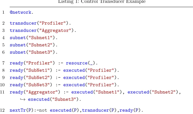
To evaluate the behaviour of the system, we used the datasets in Table 2, that comprise a mix of property data extracted from the web and curated open government data. The experiments were run on a MacBook Pro with 8GB RAM and a 2.7GHz Dual Core i5 processor, using Postgres 9.5, Java 8 and Lpsolve 5.5.
In all experiments, the target schema T consists of one table, property, with 5 attrib-utes: postcode, price, crimerank, street and city_town. The goal in each experiment is to automatically populate this schema with 1000 tuples, using data from the sources. Although providing a size for the result could sometimes be difficult for data scientists, we note that working with an unconstrained result size in automated wrangling can lead to ever lower quality tuples being included in the result; there needs to be some con-straint on the size of the end data product.
For all experiments, the sources are added incrementally in a random order (with the exception of the UK deprivation data that is always available), and this was repeated 3 times per experiment. Thus, the values plotted in Figs. 7, 8, 9, 10, 11, 12, 13, 14, 15, 16, 17 and 18 are the averages of the 3 runs.
Ground truth (GT) For the GT, an initial data product was created by manually match-ing all source attributes, and then joinmatch-ing on postocode all web extracted sources with the UK indices of deprivation dataset. We then created a dataset that forms the ground truth by sampling 1000 tuples from the complete dataset (of 10.5k tuples). Using format
Table 2 Real world datasets
Sources Size
Property sources a. Data extracted using OXPATH [42]. 40 real estate sources, 6 to 16 attributes each, an average of 11 attributes per source, 7.8k tuples in total. Used as source data
b. Wadar [43]. 10 sources, 18 varying attributes each, 3.2k tuples. Used as source data
c. Price Paid Data (www.gov.uk). Property sales in England and Wales for 2017. 16 attributes, 130 properties sold in Oxford and Manchester, sampled from 461.2k tuples. Used as example data
English indices of deprivation 6 attributes, 62.3k tuples with indices for Manchester and Oxford, from http:// www.gov.uk. Used as source data
transformation, we homogenised the street contents of the sample, based on the exam-ples generated from the Open Addresses UK dataset. CFD Miner was then trained with a
support size of 20 on the Open Addresses UK dataset and detected 516 CFDs. These gave rise to 170 violations on the sampled dataset, that were then repaired. All transformation and repair rules were manually validated before being applied.
All source tuples are annotated with provenance information at tuple level. To evaluate precision, for all tuples in the end product with the same provenance, we compare each attribute of the end product with the respective attribute in the GT. Thus, a true positive (tp) is an attribute value in the end product that is also present in the corresponding GT tuple. A false positive (fp) is an attribute value in the end product that is not equal to the one in the corresponding GT tuple. As usual, precision = fptp+tp . We do not report on recall, as our ground truth is not a complete wrangled result, but a curated sample of the end product.
Experiment results
In this section, we study system behaviour in the 4 different data wrangling scenarios, and additionally investigate self-tuning, run-time and cost-effectiveness of the approach. There is no comparison with other data preparation systems, as we know of no suitable comparator (a head-to-head comparison would require a competitor with similar scope, level of automation, and evidence for informing the automation).
Scenario 1. Bootstrap
In this experiment, we study the precision of the end product in the setting where the user only provides the target schema T and a set of sources S, and a preferred result size in tuples. There is no User Context, Data Context or feedback.
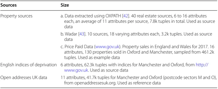
Since User Context is needed to perform mapping selection, the intuition here was that some data is better than no data (in the sense that complete tuples are better than incomplete ones), so in this case the user context consists of just one criterion with a weight of 1, tuple-completeness wrt. empty values, defined as the fraction of complete tuples in a result. Using this criterion, in Fig. 6, we experiment with the targeted size
by increasing it from 1000 tuples to 9000 tuples, and we illustrate the composition of the end product. All 50 sources are available in all cases, and the circle size of each source is proportional to the fraction of the tuples from the source that were selected to populate the end product. We notice that the system handles diversity for this cri-terion by selecting complete tuples at first from a few selected sources, but as the tar-geted size increases, it is required to select data from sources that typically contain fewer complete tuples, ultimately selecting nearly all tuples returned by the candidate mappings.
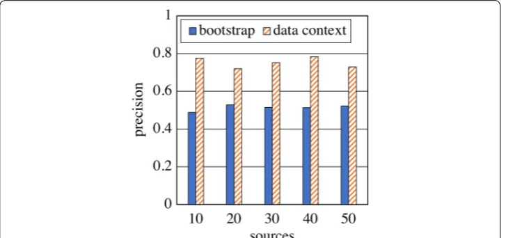
In Fig. 7, the number of sources is increased from 10 to 50, and the precision of the end product is reported in 2 cases. In the first case, bootstrap, the end product is obtained in the absence of any data context or user context. The transducers involved are matching, mapping and mapping selection. The precision of the result is not good, but the sys-tem has access to quite little information about the application, and as a result there is no instance matching, no data repair and no format transformation. The next scenario shows how this can be improved.
Scenario 2. Data context
In this experiment, Data context is added, to study the impact that it can have on the end product. This includes Price Paid data that are used as example data, and the Open Addresses UK data that are used as reference data. The addition of data context pro-vides the ability to: (a) perform instance-based matching; (b) evaluate data context-related metrics (accuracy, consistency and completeness); (c) discover transformation examples, synthesise and apply format transformations based on these examples; and (d) learn CFDs, detect violations and carry out repairs on the end product. As in the first scenario, in the absence of user context, we use the default criterion, of tuple-com-pleteness wrt. empty values, with a weight of 1. As shown in Fig. 7, adding data context leads to a substantial increase of the precision of the end product. We do not discuss data context further here, as a more comprehensive evaluation of data context is pro-vided in [23].
Scenario 3. User context
In this experiment, we study the impact of the user context on the end product. The 10 criteria used in this experiment are: completeness w.r.t. empty values applied to
street, city_town, postcode, price and crimerank; completeness w.r.t. data context
applied to street and city_town; and consistency w.r.t. data context applied to street,
city_town and postcode. In all experiments, criteria weights are set to 1
C , where C is
the number of criteria in the experiment.
The base case, plotted as 0 criteria in the graphs, is that in which there is no user-provided user context. In this case, the default criterion, tuple-completeness wrt. empty values, with a weight of 1 is used, as in Scenarios 1 and 2.
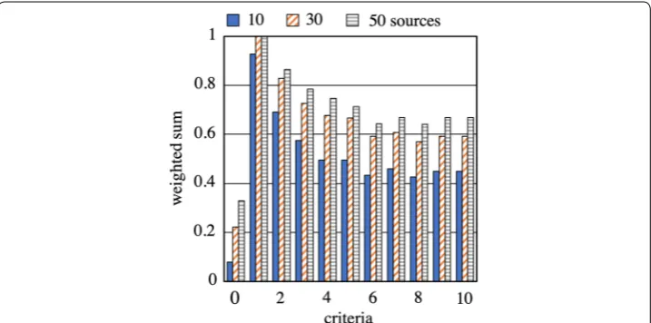
To evaluate the extent to which user requirements have been met, we can evaluate the WS (introduced in Eq. 6) of the end product. However, WS results are not compa-rable across user contexts with the same number of criteria but with different types. There may be criteria for which it is not possible to have a high value, given the data available. For instance, in our wrangling setting the criterion completeness w.r.t. data context applied to town had a maximum evaluation of 0.65 on a candidate end prod-uct. In contrast, completeness w.r.t. empty values applied to price is high in virtually all sources. The consequence of this property can be seen in the lack of a firm trend in
WS values as criteria are added in Fig. 8.
Thus, to study the outcome with respect to what is possible given the data, we intro-duce the Normalised Weighted Sum (NWS) as:
wj is the weight of criterion j, cj is the result of evaluating criterion j on the end product,
and Z∗
j (resp. Zj∗∗ ) is the ideal (resp. negative ideal) solution for criterion j, i.e. the
maxi-mum (resp. minimaxi-mum) value for this criterion if all data would be available, and if this was the only criterion in the user context.
(7)
NWS=
C
j wj
cj−Z∗∗j Z∗
j −Zj∗∗
Figures 9 and 10 show the extent to which the end product satisfies the user prefer-ences, given the data available in the system. We notice that the NWS increases while the sources increase; this is because the addition of new sources makes available addi-tional data that may be able to meet the criteria. The NWS also decreases as the num-bers of criteria increase, as with more criteria there is more need for compromise. Note, however, the low NWS for the base case (0 user-defined criteria); this shows that user context can substantially influence the suitability of the result data set.
Next, we show how the system behaves when the targeted size is increased. Fig-ure 11 illustrates the precision of the end product, the WS, and the NWS in the case when all 10 criteria in the User Context are used, and in the base case, when only the default criterion, tuple-completeness w.r.t. empty values, with a weight of 1 is used, as in Scenarios 1 and 2. The setting in this experiment is the same as in Fig. 6. The num-bers in parentheses in Fig. 11 refer to the number of the user-defined criteria, where 10 are all the criteria listed in this section, and 0 is the base case. Precision, the WS and the NWS are plotted for both these cases.
Fig. 9 Scenario 3. Normalised weighted sum for different numbers of criteria
In the base case, using the default criterion, tuple-completeness w.r.t. empty values, with a weight of 1, may lead to a decreasing WS as the targeted size increases, but NWS is always at 1, meaning that at all times all complete tuples available in the sys-tem were being selected to populate the end product.
In the case of 10 criteria, the WS (10) also decreases, as the system is forced to select more tuples, even when these are of lower quality. However, at all times, the NWS is maintained above 80%, meaning that the system outcome, though trading off different criteria, is consistently close to what is possible with the data available. Also, maintaining a high precision means that the application of user context did not sacrifice correctness.
In all the above, it is shown that the system provides consistent behaviour when either the amount of source data available increases, or the amount of data in the end product increases.
Scenario 4. Feedback
In this scenario, we study the impact of user feedback on the end data product in a pay-as-you-go manner. The user can provide feedback on tuples or their attribute values. User feedback is simulated by adding incrementally up to 500 feedback instances (f.i.) on the relevance of tuples or attribute values in the end data product, randomly annotating them as relevant or not. The complete data set contains 1000 tuples and 5 attributes, so
500 feedback instances (250 on tuples and 250 on attribute values) correspond to feed-back on 30% of the overall result size. The User Context comprises 5 criteria, each of which is of type relevance, and has a weight of 0.2. The relevance of an attribute M.a of a candidate mapping M is calculated as:
(8)
RelevanceM.a=
1
2(1+
tpM.a−fpM.a
tpM.a (resp. fpM.a ) are the numbers of true (resp. false) positives provided by user feed-back, and |M.a| is the number of attribute values. When there is no feedback on the mapping, the default relevance is 0.5, which represents unknown relevance. User feed-back is propagated in the candidate mappings as follows: when the user marks a tuple as a tp, its constituent values are marked as tp when evaluating relevance on the candidate mappings. Accordingly, when an attribute value is marked as a fp, all tuples containing the value are marked as fp.
Figures 12 and 13 show how the relevance, represented as the WS (Eq. 6), of the end product increases as more sources and more user feedback become available in the sys-tem. We report the WS, as there is no need for normalisation; relevance can take any value between 0 and 1. As we can see, for 50 sources, the WS of the end product will be higher than in the case of 30 or 10 sources, as there is more potentially relevant data available. Similarly, the weighted sum of the end product keeps increasing as more feed-back instances are obtained, though at a diminishing rate. This is because the impact of propagated feedback instances is high at first but decreases as the estimates of source
Fig. 12 Scenario 4. Weighted sum for different amounts of feedback
quality become dependable, and thus tend to change little when more feedback is obtained.
Self-tuning In this set of experiments we evaluate the impact of parameter self-tuning on result suitability. Here, instead of setting the parameters of wrangling components manually, different parameter values were experimented with in different transducer subnetworks, as shown in Figs. 14 and 15. We considered 3 User Contexts for self-tun-ing experiments: User Context 1 contains all 10 criteria that were used in the User Con-text experiment, User Context 2 the first 6, and User Context 3 the last 3 criteria. As in the User Context experiments, criteria weights are set to 1
C , where C is the number of criteria.
The empirically chosen parameters led to the subnetworks 1–9, which respectively are configured with match thresholds of 0.5, 0.6 and 0.7, and support sizes for CFD Miner of 20, 40 and 60 tuples. As such, the parameters for match threshold and support size for the 9 subnetworks in Figs. 14 and 15, are respectively (0.5,20), (0.6,20), (0.7,20), (0.5,40), (0.6,40), (0.7,40), (0.5,60), (0.6,60) and (0.7,60). Using the same 30 sources at all times, the execution of each of the subnetworks created a candidate end product. The Aggregator selects the one that produces the highest WS, as this should most closely correspond to the user’s preferences.
For each of the three user contexts, the selected candidate end product is marked with a bold outline in Fig. 14. The best result is achieved with different parameter combina-tions in each case. For User Context 1, the end product with the highest WS is obtained by subnetwork 8, for User Context 2 by subnetwork 1, and for User Context 3 by subnet-work 7.
Next, we experimented using the same User Context while modifying the number of sources. The filled markers in Fig. 15 highlight the best result in each case. We can see that subnetworks 4, 1 and 2 give the best results for 10, 30 and 50 sources, respectively. These results show that the most suitable configuration parameters are sensitive to spe-cific user contexts, and thus that they are likely to be extremely difficult to set manually, demonstrating the potential significance of self-tuning.
Scenario runtimes Figure 16 shows the average time experiments took to run to com-pletion. In Fig. 16, the setting is as in the 4 scenarios previously described. Bootstrap and data context scenarios consist only of the default user context (tuple-completeness wrt. empty values). For the user context scenario, we include all 10 criteria, and in the feed-back scenario there are 25 feedfeed-back instances.
The increase in runtime when adding data context, compared to bootstrap, happens because the system can (a) perform instance-based matching, (b) generate examples to synthesise transformations, and (c) learn CFDs in order to repair the candidate end product. As sources increase, instance-based matching and examples generation (for scenarios 2, 3, and 4) take place on more sources, and the number of inclusion depend-encies and candidate keys increases, presenting a larger number of join opportunities to consider for mapping generation. The runtime of mapping selection and data repair is not affected because the maximum number of candidate mappings k is always set to 100, and data repair is only applied to the candidate end products.
Fig. 15 Self tuning. Weighted sum for different numbers of sources
We notice that the feedback scenario is the most expensive, as it includes evaluation of the relevance for each of the 5 attributes of the target schema, in addition to the expen-sive propagation of all feedback instances to all candidate mappings. Thus, because of propagation, the feedback scenario is slightly more expensive than the User Context scenario, even though 5 criteria are evaluated in the former, rather than 10 in the lat-ter. Finally, we see that even though criteria evaluations run in parallel, the user context scenario is slightly more expensive than the data context scenario that only contains one criterion.
Manual effort estimation Next, while recognising that there is no one-size-fits-all when it comes to estimating data preparation, we obtained an estimation of the time it would take to manually wrangle the sources in our scenarios, using the default values of the EFES open source tool [24]. As illustrated in Fig. 17, whether a low-effort result is acceptable, or a higher quality result is required, preparing the sources is estimated to take up to several hours of a data scientist’s time.
Scaling the number of sources To test how the system performs on a large number of sources, we created copies of the source data (a and b in Table 2), and introduced ran-domness in their number of columns, column names and instances, so as to obtain a total of 1k sources. We then ran the 4 scenarios as before, while increasing the number of sources, and show the results in Fig. 18. We notice that the runtime remains below 5 minutes for up to 600 sources. The feedback scenario is still slightly more expensive than the others.
In Fig. 19, we show a breakdown of the components that ran in the experiment in Fig. 18, in the case when data context is available. Overall, when scaling the number of sources, the mapping generation transducer scales the least well. Although we apply sev-eral pruning strategies within the dynamic programming, mapping generation is faced with a need to search an increasing space of potential mappings; for instance, in the case of 1k sources in the data context scenario, the mapping generation transducer had to consider join/union opportunities arising from approximately 11.8k inclusion depend-encies (with overlap threshold set to 0.8), and 2.9k matches (with a threshold set to 0.6).
We note, however, that the system can accommodate significant numbers of sources, and that for applications in which there are very large numbers of available sources, such as in data lakes, some form of initial source selection should be able to be applied (e.g. [25]).
Drilling down further, in Fig. 20 we can see the CPU and RAM consumption, when a scenario is run on one computer, in the case when 300 sources are wrangled in the pres-ence of data context, as in the experiments in Fig. 6. The scenario terminates in 170 s. The CPU reported is the actual CPU load on the machine, while as RAM we report on the load of the memory available to the JVM, currently set at 1.82 GB. The dotted ver-tical gray lines show when the execution of a transducer terminates, and the next one starts. Specifically, in this experiment, we see that for the first 12 s the system initialises, i.e. it collects metadata about the available sources. Then the match transducer runs an instance-based match for the next 39 s (12 to 50). Profiling then runs for 44 s (51 to 94),
Fig. 18 Large numbers of sources. Runtimes for large numbers of sources
mapping generation for 53 s (95 to 147), and mapping selection for 16 s (148 to 163). Finally, it takes 3 s (164 to 166) for the CFD Miner, Violation detection, and Rule-based repair transducers to run, and another 3 s (167 to 169) for the Aggregator to finalise the scenario.
CPU load bursts occur when tasks run in parallel, as in the case of instance-based matching, profiling and mapping selection. Memory usage drops near the end of the Matching and the Profile transducers because most of the initial threads within the transducer have run to completion.
Discussion
In this section, we consider related work on Data Preparation Platforms and on Auto-mating Data Preparation. In relation to Data Preparation Platforms, there are several widely adopted approaches; here we classify proposals into view-based data integration,
extract–transform–load (ETL) and interactive data reformatting.
In view-based data integration, as represented in the literature by systems such as Clio [26] and ++Spicy [27], data engineers curate matches and mappings, with a view to producing high quality integrated databases, typically over sources that are themselves enterprise databases [28]. The foundation of such systems in database queries can addi-tionally enable their integration with declarative repair techniques, as supported by sys-tems such as BigDansing [29], Nadeef [30] and Llunatic [31]. However, although such approaches enable the production of good quality results, this comes at the cost of sig-nificant manual input from data engineers to refine the matches, mappings and quality rules that together lead to the population of a data product.
Data integration for data warehouses often makes use of ETL platforms [32], in which processes are authored by data engineers, who identify and configure the operations required to populate the target, making explicit their dependencies in a workflow. Such systems often provide substantial libraries of integration functions, and a visual edi-tor for workflow authoring. Their utility is reflected in a significant number of success-ful products, but data engineers retain fine-grained control over specification tasks,
reducing the utility of ETL platforms for applications with many or rapidly changing sources. Although approaches have been proposed that enable the system to take more responsibility for optimization [2], the primary decisions on how data is prepared are hand crafted. The data preparation steps carried out in VADA provide functionalities that have similar scope to those found in ETL systems, and as such VADA provides evi-dence as to how greater automation could be made available in ETL platforms.
Less focused on enterprise data sets, platforms that support interactive data reformat-ting, such as OpenRefine and Wrangler [3], support authoring of format transformation scripts over tabular data representations, often providing suggestions for how to author transformation rules based on examples. Such approaches are now supported by several products (e.g., Trifacta, Talend Data Preparer). In these approaches, however, although the tools support the authoring of transformations, it is still up to users to engage in the creation of individual transformations by providing examples, validating or refining rules, and to handcraft the data processing pipeline.
As such, most work on data preparation platforms supports data engineers in pro-gramming for data integration, rather than providing a central role for automation. In relation to Automating Data Preparation, there are many results, though mostly focused on individual data preparation steps. For example, well known algorithms and platforms exist that can be used to automate matching (e.g. [33]), mapping generation (e.g. [26, 27]) and format transformation (e.g. [20, 34]). Indeed, in this work we build on approaches that automate individual data preparation steps. However, the contribu-tion of this paper is not so much in the individual steps; instead, our approach has been to provide an architecture in which a complete data preparation process is automated, benefitting from cross-cutting capabilities such as dynamic orchestration, data context to inform individual steps, user context to choose between integrations, and feedback to refine results. Indeed, feedback is often used in conjunction with automated compo-nents (e.g. as reviewed in [35, 36]), but again typically in the context of individual data preparation components.
options; SemLinker can be seen as providing a graph through which different data sets can be accessed, whereas VADA can be seen as automating the authoring of ETL flows. There are no direct analogues of data context or user context in SemLinker, and indi-vidual data sets are subject to fewer synthesised transformations; for example, there is no data repair.
Conclusions
Here we revisit the claimed contributions from the introduction, in the light of the details in the paper. The claimed contributions are:
a. An architecture in which loosely coupled data preparation components are declar-atively and dynamically orchestrated. The architecture supports data preparation components for matching, data profiling, mapping generation, format transforma-tion and data repair, represented as transducers, and orchestrated using policies specified in Vadalog. Orchestration dynamically selects different transducers to par-ticipate in the wrangling process based on the information available in the knowledge base, and control transducers can explore alternative configuration parameters for self-tuning. The overall effect is that the user specifies what is required and the sys-tem determines how this should be produced.
b. An approach to automating data preparation that takes into account user prefer-ences and user feedback. The central role of automation in the architecture means that many alternative candidate data products can be produced. To align these to the requirements of the user, pairwise comparisons of quality criteria can be used, and both criteria and their weights can be revised to steer the solution towards the pref-erences of the user. Furthermore, as automation cannot be sure to identify correct or relevant results, feedback from the user can support the evaluation of additional criteria, revising the choice of candidate mappings from which results are obtained. c. An evaluation of the resulting approach. The evaluation results show that the data
wrangling components, when provided with suitable data context data, can automat-ically produce results with precision above 0.7, that the multi-criteria mapping selec-tion can produce results with much higher utility than data selected using generic criteria, that self-tuning of parameter values across several components can have a significant impact on the utility of the results, and that the approach can wrangle hundreds of sources in minutes—a scale of data preparation activity that would likely take a data scientist many days of manual effort.
Several areas for future work suggest themselves. In relation to the result of the data preparation process, it would be possible to investigate how automated data preparation could be informed by target schemas that are designed to be used with specific types of analysis, either informed by machine learning tools or data warehouses. The additional information about the target could, for example, be reflected in mapping generation and mapping selection.