ORIGINAL RESEARCH
DeepNeuron
: an open deep learning
toolbox for neuron tracing
Zhi Zhou
1,2, Hsien‑Chi Kuo
1, Hanchuan Peng
1,2*and Fuhui Long
1*Abstract
Reconstructing three‑dimensional (3D) morphology of neurons is essential for understanding brain structures and functions. Over the past decades, a number of neuron tracing tools including manual, semiautomatic, and fully auto‑ matic approaches have been developed to extract and analyze 3D neuronal structures. Nevertheless, most of them were developed based on coding certain rules to extract and connect structural components of a neuron, showing limited performance on complicated neuron morphology. Recently, deep learning outperforms many other machine learning methods in a wide range of image analysis and computer vision tasks. Here we developed a new Open Source toolbox, DeepNeuron, which uses deep learning networks to learn features and rules from data and trace neu‑ ron morphology in light microscopy images. DeepNeuron provides a family of modules to solve basic yet challenging problems in neuron tracing. These problems include but not limited to: (1) detecting neuron signal under different image conditions, (2) connecting neuronal signals into tree(s), (3) pruning and refining tree morphology, (4) quantify‑ ing the quality of morphology, and (5) classifying dendrites and axons in real time. We have tested DeepNeuron using light microscopy images including bright‑field and confocal images of human and mouse brain, on which DeepNeu-ron demonstrates robustness and accuracy in neuron tracing.
Keywords: DeepNeuron, Deep learning, Neuron tracing, Neuron morphology
© The Author(s) 2018. This article is distributed under the terms of the Creative Commons Attribution 4.0 International License (http://creat iveco mmons .org/licen ses/by/4.0/), which permits unrestricted use, distribution, and reproduction in any medium, provided you give appropriate credit to the original author(s) and the source, provide a link to the Creative Commons license, and indicate if changes were made.
1 Introduction
Over the past few decades, researchers have developed algorithms and tools to reconstruct (trace) 3D neuron morphology. A number of manual/semiautomatic neuron tracing software packages in both the public domain and commercial world have been developed [1–9]. To fur-ther promote the development of neuron tracing tools, the DIADEM challenge [10] and the BigNeuron pro-ject [11] were launched to compare different automated algorithms. At small or medium scales, many algorithms (base tracers) have been shown to produce meaning-ful reconstructions on high-quality neuron images. For large-scale image datasets, UltraTracer [12] provides an extendible framework to scale up the capability of these base tracers. Despite these efforts on algorithm and tool development, it remains an open question on how to
faithfully reconstruct neuron morphology from challeng-ing image datasets that have medium to low qualities and contain very complex neuron morphology.
Starting from a cell body, a neuron tracing process usu-ally follows dendrites and axons, eventuusu-ally connecting all such neuron signal as a tree that represents the mor-phology of the neuron. In light microscopy images, den-drites typically show continuous signal, whereas axons are often hard to trace due to their punctuated appear-ance and large, complex arborization patterns ([8]; see for example the bright-field images of biocytin-labeled neu-rons in the Allen Cell Type Database [24]). In addition, the image quality varies a lot depending on sample prepa-ration, imaging process, cell types, and the healthiness of neurons. For instance, neuron signal could be continuous in one image, but dim and broken in another. It is difficult to automatically extract all such neuron signal under dif-ferent conditions.
Several important steps in neuron tracing can be for-mulated as a classification problem. For example, detec-tion of neuron signal from background is essentially
Open Access
*Correspondence: [email protected]; fuhuil@alleninstitute. org
1 Allen Institute for Brain Science, Seattle, USA
foreground–background classification. Reconstruction of the topology of a neuron via connecting neuron frag-ments can be treated as connection-separation classi-fication. In this aspect, a few studies used traditional machine learning and recent deep learning [13] mod-els to produce neuron morphology. For example, Gala et al. introduced an active learning model by combin-ing different features to automatically trace neurites [14]. Chen et al. proposed a self-learning-based trac-ing approach, which did not require substantial human annotations [15]. Fakhry et al. [16] and Li et al. [17] used deep learning neural networks to segment elec-tron and light microscopy neuron images. Despite these algorithmic efforts, none of these methods provides publicly available tools to use on external datasets.
Nowadays, deep learning methods outperform tradi-tional methods in many pattern recognition and com-puter vision applications. We analyzed commonly used modules of neuron tracing/editing workflows in real applications, and concluded that an Open Source deep learning toolbox would help this growing field. Using deep learning neural networks as the classification models, we develop DeepNeuron, which provides sev-eral essential modules to neuron tracing. For auto-mated tracing, DeepNeuron can be used as either a new tracing algorithm to reconstruct neurites from difficult neuron images, or an extra processing component to improve other tracing algorithms. DeepNeuron could
also assist annotators in manual tracing. Supporting extendable functions as plugins, currently DeepNeuron
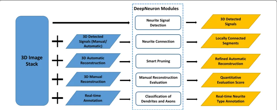
contains five commonly used modules (Fig. 1):
• Neurite signal detection automatically identifies 3D dendritic and axonal signal from background.
• Neurite connection automatically connects local neu-rite signal to form neuronal trees.
• Smart pruning filters false positive and refines auto-mated reconstruction results.
• Manual reconstruction evaluation evaluates manual reconstructions and provides quality scores.
• Classification of dendrites and axons automatically classifies neurite types during real-time annotation.
2 Five modules
2.1 Neurite signal detection
Due to difficulties in sample preparations and imaging, neurite signals often appear broken in a 3D image. It is hard to use any existing automated tracing algorithm to reconstruct 3D neuronal structures when this hap-pens. Even for human annotators, locating these isolated axonal signals from the noisy background is a daunting work. To reliably detect neurite signals, we introduce the neurite signal detection module based on deep CNN to classify signal and background. This allows us to precisely detect neurite signals without any preprocessing steps applied on the original image. To speed up the detection
Neurite Signal Detection
3D Detected Signals
3D Detected Signals (Manual/
Automatic) Neurite Connection
Locally Connected Segments
3D Automatic
Reconstruction Smart Pruning Refined AutomaticReconstruction
3D Manual
Reconstruction Manual ReconstructionEvaluation Evaluation ScoreQuantitative 3D Image
Stack
Real-time
Annotation Dendrites and AxonsClassification of Real-time NeuriteType Annotation
DeepNeuron Modules
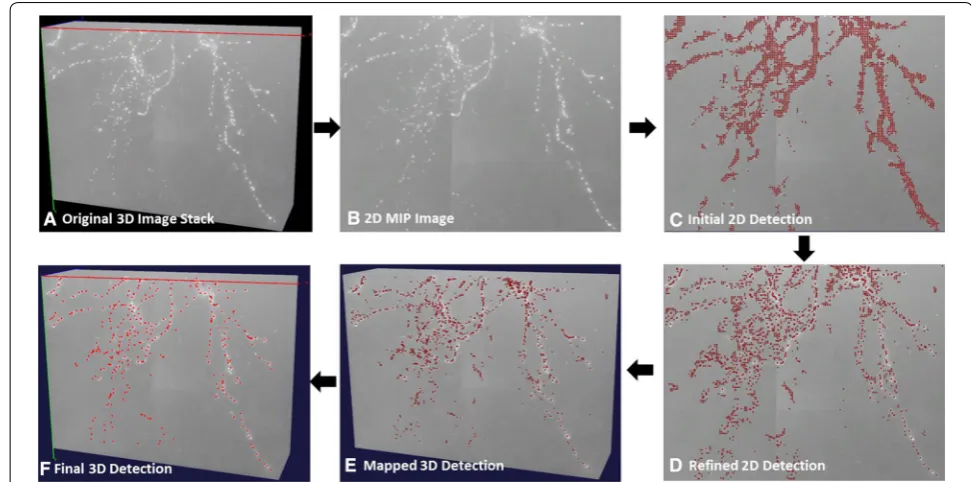
and lower the GPU memory requirement, we used a two-dimensional (2D) CNN model followed by 3D mapping to detect signal in 3D and achieved satisfactory results on our testing data. However, our framework is not limited to 2D CNN but can also directly use 3D CNN models (Fig. 2).
Manually reconstructed neurons were used as train-ing samples. The 3D reconstruction of a neuron is rep-resented as a tree, which contains a series of 3D X, Y, Z locations, radius, and topological “parent” of annota-tion nodes. To train the network, local 3D blocks (block size 61 × 61 × 61 was used in our experiments) centered on manually annotated nodes in neurite segments were
cropped from the original images. 2D maximum inten-sity projections (MIPs) of theses 3D blocks were used as the positive training set, and the same number of 2D background MIPs were randomly selected as the negative training set.
We tested our module using AlexNet [18] with five convolutional and three fully connected layers. Table 1
shows the fivefold cross-validation test of the module robustness. The training image dataset was partitioned into five equal size subsets (1–24, 25–48, 49–72, 73–96, and 97–122 as shown in Table 1). Four subsets were used for training, and the remaining single subset was used for
Fig. 2 The workflow of 3D neurite signal detection. (a) An example of the original 3D image stack. It is a cropped 3D bright‑field image of a biocytin‑labeled mouse neuron; the pixel resolution is 0.14 um × 0.14 um × 0.28 um. (b) 2D MIP on the XY plane. (c) Initial neurite signal detected by a deep CNN model (AlexNet in this case). (d) Refined 2D signal detection result using a mean shift. (c) and (d) are overlaid on top of B. (e) Mapped 3D detection result based on local maximum intensity along Z‑direction. (f) Final 3D detection result after deep learning‑based refinement. (e) and (f) are overlaid on top of (a). Red dots indicate 2D/3D detected signals
Table 1 Fivefold cross-validation on bright-field training sets
Training set Foreground accuracy Background accuracy Overall accuracy
Training (%) Validation (%) Training (%) Validation (%) Training (%) Validation (%)
{1–122}\{1–24} 98.77 97.78 98.97 96.87 98.87 97.33
{1–122}\{25–48} 98.54 99.07 98.78 98.34 98.66 98.71
{1–122}\{49–72} 98.67 98.28 98.78 99.13 98.73 98.71
{1–122}\{73–96} 98.71 96.64 98.28 99.23 98.50 97.94
{1–122}\{97–122} 98.64 99.02 98.77 98.41 98.71 98.72
validation. Our results show our overall accuracy > 98% for both training and validation.
In testing, we first projected the original 3D image stack onto the XY plane and generated a MIP image. We then cropped 2D patches using a sliding window with
n-pixel stride. These patches were classified into patches centered on foreground or background pixels using our trained CNN model. To further improve classification accuracy and exclude false positive patches, we applied mean shift [19] to the detected foreground patches and map them back to the actual 3D locations based on the local maximum intensity along Z. Finally, we classified these 3D detected signals using our CNN model again based on the MIPs of the local 3D blocks.
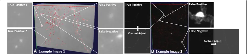
We applied our module to two challenging datasets of mouse neurons. The first set was a bright-field biocy-tin-labeled mouse neuron dataset from Allen Cell Type Database [24]. The second set was a whole mouse brain data imaged by fMOST imaging technology [20]. For the first dataset, we used 122 bright-field neuron image stacks and their associated manual reconstructions as the training set and produced ~ 813 K training samples including ~ 404 K foreground patches, and ~ 408 K back-ground patches. For the whole mouse brain dataset, we used ~ 493 K training samples including ~ 252 K fore-ground patches, and ~ 241 K backfore-ground patches from 22 whole mouse brain images. Figure 3 shows two exam-ples of axon detection results. Using neurite signal detec-tion module, most of axonal signals have been precisely detected in both datasets.
2.2 Neurite connection
A complete neuron forms a tree structure that is com-posed of continuous neurite segments. Global, local, and topological features including total length, bifurcations, terminal tips, and more others are used to study the neu-ronal morphology. These features have to be extracted
from neurite segments instead of dots. Therefore, find-ing the continuity of neurites and connectfind-ing neurite segments are critical steps in neuron tracing. Generally, automated tracing algorithms can achieve good perfor-mance on connecting neurite segments with small gaps based on the continuity of segment orientations. How-ever, it is difficult to automatically connect dots-like neurite signals. Using the spatial distance between these signals as the weight, minimal spanning tree (MST) provides a possible solution. However, without biologi-cal context, it could also introduce topologibiologi-cal errors. Human beings are good at finding the continuity of iso-lated signals as per their observations and domain knowl-edge. By learning the neurite connectivity from a large dataset annotated by humans, a deep learning-based MST (DMST) approach we proposed can successfully connect neurite segments with relatively big gaps (Fig. 4).
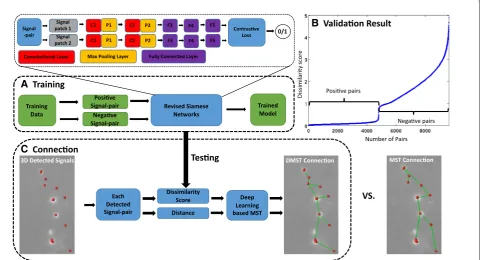
Siamese networks [21, 22] are used among tasks that involve finding similarity or the relationship between two subjects being compared. Our revised Siamese model in this work includes two identical arms. Each consists of two convolutional layers with max pooling, followed by three fully connected layers. The two arms are then fed to a contrastive loss function to produce a binary decision.
In training (Fig. 4a), we used pairs of patches generated from two consecutive annotation nodes as positive train-ing samples, and pairs of patches generated from two spatially separated annotation nodes as negative training samples. We used ~ 919 K training pairs, ~ 460 K of them being positive pairs and ~ 459 K being negative pairs.
In connection (Fig. 4c), a 1 × M feature vector is extracted from individual input patch. (M can be defined by the user, and we used M= 200 in our experiment.) The Euclidean distance between two feature vectors is calcu-lated as the dissimilarity score of a patch pair, which is multiplied by the distance to form the weight in our pro-posed DMST graph.
B Example Image 2
False Posive
False Negave
False Posive
False Negave
Contrast Adjust
True Posive 1
True Posive 2
True Posive
Contrast Adjust
A Example Image 1
Training Data
Posive Signal-pair
Negave Signal-pair
Trained Model
Each Detected Signal-pair
Dissimilarity Score Distance
Deep Learning based MST A Training
C Connecon
3D Detected Signals DMST Connecon MST Connecon
VS.
Dissimilarity
sco
re
Posive pairs
Negave pairs
B Validaon Result
Revised Siamese Networks
Signal -pair
Signal patch 1 Signal patch 2
C1 P1 F3
Contrasve Loss C2 P2 F4 F5
Convoluonal Layer Max Pooling Layer Fully Connected Layer C1 P1 C2 P2 F3 F4 F5
0/1
Number of Pairs
Tesng
Fig. 4 The workflow of neurite connection module. (a) In the training step, the connectivity of a signal pair is learned using a revised Siamese network. In each pair, two 1 × 200 feature vectors are extracted. (b) The validated result with sorted dissimilarity scores for all signal pairs shows that the dissimilarity scores of positive pairs are much lower than that of negative pairs. (c) The trained model is applied in the connection step to calculate the dissimilarity for each detected signal pair. Results of our DMST connection and the original MST connection (using distance as the weight only) are shown
Combing neurite signal detection and neurite connec-tion modules, we were able to reconstruct axons that present big challenges to traditional methods due to large gaps between signal segments (Fig. 5).
2.3 Smart pruning
Many of the existing automatic tracing algorithms rely on the correct estimation of the threshold that separates the potential foreground signal from the background. Typi-cal methods include those that use the weighted aver-age intensity of the entire imaver-age to threshold the imaver-age or add a preprocessing step to enhance signals. These methods have limited success for neuron images with low signal-to-noise ratio and uneven background. To solve the problem, we developed a smart pruning module in
DeepNeuron. It relieves the burden of precisely separat-ing foreground and background up the front. Usseparat-ing exist-ing algorithms, our module first generated over-traced results with a lower foreground/background segregation threshold or through signal enhancement step. We then trained CNN networks to classify true signals and false positive signals. Using the trained models, we filtered out falsely detected signals and pruned the reconstructed
neuronal tree. Furthermore, different tracing results gen-erated from multiple base tracing algorithms could be combined [23] to produce a consensus using this module (Fig. 6).
2.4 Manual reconstruction evaluation
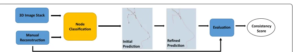
Since manual reconstruction is largely used as the gold standard to evaluate automated reconstruction algo-rithms and to generate training set for machine learn-ing-based approaches, it is important to assess the consistency of manual reconstructions among different annotators or of the same annotator at different times. For this purpose, DeepNeuron provides an evaluation module based on deep learning classification model. Take the mouse neuron dataset from the Allen Cell Type Database [24] we described in Sect. 2.1 as an example, we divided the 122 manual reconstructions from multi-ple annotators into five subsets and took a fivefold cross-validation strategy. Each time we took four subsets as the training data. Once the network was trained, we used it to evaluate how consistent the remaining subset is with respect to the training subsets (Fig. 7, Table 2). More specifically:
Fig. 6 The workflow of consensus generation using the smart pruning module. Multiple automatic reconstructions are filtered by CNN‑based classification models first. Then, all filtered reconstructions are fused together to produce a consensus. Reconstructions are shown in red lines on top of the original image stack
Node Classificaon Manual
Reconstrucon 3D Image Stack
Evaluaon
Inial Predicon
Refined Predicon
Consistency Score
• First, all annotation nodes in test subset were classi-fied into two categories: foreground and background.
• All classified foreground nodes formed an initial pre-diction.
• Based on the orientation, tip location, and distance, fragments in the initial prediction were automati-cally connected to produce a refined prediction. In our experiment, we only connected terminal tips between two segments whose orientation differs less than 30 degrees and distance is smaller than 30 vox-els.
• The test subset is evaluated by the consistency score
c:
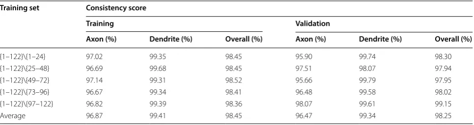
Table 2 shows the fivefold cross-validation results on 122 manual reconstructions for the bright-field biocy-tin-labeled mouse neuron dataset from Allen Cell Type Database [24]. The high consistency scores indicate that manual reconstructions are very consistent across dif-ferent annotators and difdif-ferent subsets of data. In addi-tion, thicker and more continuous dendrites (> 99%) have higher consistency scores than dim and discontinuous axons (> 96%), which are harder to reconstruct.
More broadly, we applied our evaluation module to 31 manual reconstructions including 10 human neurons and 21 mouse neurons in the Allen Cell Type Database [24].
c= Number of nodes in the refined prediction
Number of nodes in the manual reconstruction×100%
Table 3 shows our comparison results. Consistent with Table 2, dendrites have higher scores than axons. In addi-tion, scores on human neurite (axon and dendrite) recon-structions are higher than those of mouse, indicating that annotators have better tracing performance on physically larger human neurons.
2.5 Classification of dendrites and axons
Dendrites and axons have their own functions and play different roles in the nervous system. Distinguishing these two types of neurites can help us gain insight into the brain circuitry. Although dendrites and axons show different shapes and intensity properties in light micros-copy images, such a general rule of thumb, however, is not always guaranteed. Due to variant image qual-ity, axons can also appear continuous and look more like dendrites. This makes them difficult to be correctly labeled in most of tracing algorithms. Here we present a deep learning module serving as a vehicle for the net-works that are trained for this purpose. This tool allows to automatically classify dendrites and axons on real-time manual annotation, and potentially save real-time for annotators.
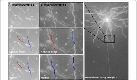
We used the same approach as described in Sect. 2.1, except that the problem is now a multinomial classi-fication (dendrite, axon, and background) instead of a binary classification (foreground and background) problem. Figure 8 shows the performance on two test-ing cases from the Allen Cell Type Database [24]. In this example, we used ~ 813 K training samples includ-ing ~ 143 K axons, ~ 261 K dendrites, and ~ 409 K back-ground. In this article, AlexNet and a revised model were used as demonstration. In Fig. 8, both AlexNet and our revised model can accurately classify con-tinuous dendritic and discrete axonal signals. How-ever, when the signal of axons is similar to dendrites (Fig. 8b), AlexNet mistakenly classified axons into den-drites, while the revised model with one more convo-lutional layer successfully distinguished axons from Table 2 Fivefold cross-validation on 122 manual reconstructions of biocytin-labeled mouse neuron dataset
Training set Consistency score
Training Validation
Axon (%) Dendrite (%) Overall (%) Axon (%) Dendrite (%) Overall (%)
{1–122}\{1–24} 97.02 99.35 98.45 95.90 99.74 98.30
{1–122}\{25–48} 96.69 99.68 98.45 97.51 98.07 97.94
{1–122}\{49–72} 97.14 99.31 98.52 95.66 99.79 97.95
{1–122}\{73–96} 96.67 99.34 98.41 96.48 99.58 98.02
{1–122}\{97–122} 96.82 99.39 98.36 98.07 99.61 99.15
Average 96.87 99.41 98.45 96.47 99.34 98.25
Table 3 Comparison results of consistency scores on human and mouse neuron reconstructions
Number Axon (%) Dendrite (%) Overall (%)
Human 10 98.23 99.60 98.93
dendrites. Table 4 shows the comparison of classifica-tion accuracy between the two models on the training samples. We found that the revised model yields much better classification performance. In exchange, the effi-ciency of the revised model is sacrificed due to much more number of outputs in each convolutional layer (3.27-s forward–backward time for AlexNet; 335.91-s forward–backward time for the revised model).
3 Discussion
In this paper, we presented a new deep learning-based Open Source toolbox for neuron tracing: Deep-Neuron. With extensible framework, DeepNeuron
currently provides five modules to comprehend the major tasks:
• For a neuron image stack, it can be used to automati-cally detect neurite signals.
• For a neuron image stack with detected 3D signals, it can automatically connect signals to generate local segments.
• For a neuron image stack with its associated auto-mated reconstruction, it can be used as a filter to clean up all false positive tracing and generate a refined result.
• For a neuron image stack with its associated manual reconstructions, it can evaluate how consistent and reliable the reconstructions are.
• For a neuron image stack with interactive human annotation via the user interface, it can label neurite types in real time.
Fig. 8 Comparison of dendrite and axon classification using AlexNet and a revised model. (a) Axons are discrete, and dendrites are continuous. (b) Both axons and dendrites are continuous. The left segment is extracted from a long axon. The right segment is extracted from a local dendrite. Red color indicates the axon, and blue color indicates the dendrite in (a) and (b). Note that all these 3D segments are manually annotated using Virtual Finger technology [7, 9]; neurite types are automatically annotated by the proposed module
Table 4 Comparison of AlexNet with a revised model
Deep learning
network Averaged forward– backward time (s)
Deemed axon (%)
Deemed dendrite (%)
Deemed background (%)
AlexNet 3.27 84.79 93.86 99.04 A revised
DeepNeuron has been implemented as an Open Source plugin in Vaa3D (http://vaa3d .org) [7, 8]. DeepNeuron
toolbox is a highly flexible vehicle allowing investigators to take advantage of deep learning to facilitate neuron tracing in their research. As mentioned in this article, researchers can freely replace different network mod-els that suit their needs. Combined with other related features in Vaa3D including 30+ automatic neuron tracing plugins, semiautomatic neuron annotation, anno-tation utilities, neuron image/reconstruction visualiza-tion, DeepNeuron works as a smart artificial intelligence engine which offers great help to biologists in exploring neuronal morphology.
4 Toolbox and software availability
The DeepNeuron toolbox was written in C++ as a plugin to Vaa3D. DeepNeuron source code is available at https :// githu b.com/Vaa3D /vaa3d _tools /tree/maste r/hacka thon/ MK/DeepN euron . In addition, the DeepNeuron plugin is also included as a plugin in binary releases of Vaa3D, which can be downloaded at https ://githu b.com/Vaa3D / Vaa3D _Data/relea ses/tag/1.0.
Authors’ contributions
HP conceived and managed the project. FL proposed the overall technical framework. ZZ developed the toolbox and conducted the experiments. HK implemented a plugin for the dendrite and axon classification and assisted in several other experiments. All authors edited the manuscript. All authors read and approved the final manuscript
Author details
1 Allen Institute for Brain Science, Seattle, USA. 2 Southeast University – Allen
Institute Joint Center for Neuron Morphology, Southeast University, Nanjing, China.
Acknowledgements
We thank Allen Institute for Brain Science for providing neuron datasets and manual annotations. The authors wish to thank the Allen Institute founders, P. G. Allen and J. Allen, for their vision, encouragement, and support.
Competing interests
On behalf of all authors, the corresponding author states that there is no competing interests.
Ethics approval and consent to participate Not applicable.
Publisher’s Note
Springer Nature remains neutral with regard to jurisdictional claims in pub‑ lished maps and institutional affiliations.
Received: 26 February 2018 Accepted: 18 April 2018
References
1. Choromanska A, Chang S‑F, Yuste R (2012) Automatic reconstruction of neural morphologies with multi‑scale tracking. Front Neural Circuits 6:25
2. Donohue DE, Ascoli GA (2011) Automated reconstruction of neuronal morphology: an overview. Brain Res Rev 67:94–102
3. Feng L, Zhao T, Kim J (2015) neuTube 1.0: a new design for efficient neuron reconstruction software based on the SWC format. eNeuro 2:ENEURO‑0049
4. Longair MH, Baker DA, Armstrong JD (2011) Simple neurite tracer: open source software for reconstruction, visualization and analysis of neuronal processes. Bioinformatics 27:2453–2454
5. Luisi J, Narayanaswamy A, Galbreath Z, Roysam B (2011) The FARSIGHT trace editor: an open source tool for 3‑D inspection and efficient pattern analysis aided editing of automated neuronal reconstructions. Neuroin‑ formatics 9:305–315
6. Meijering E, Jacob M, Sarria JC, Steiner P, Hirling H, Unser M (2004) Design and validation of a tool for neurite tracing and analysis in fluorescence microscopy images. Cytom Part A 58:167–176
7. Peng H, Bria A, Zhou Z, Iannello G, Long F (2014) Extensible visualiza‑ tion and analysis for multidimensional images using Vaa3D. Nat Protoc 9:193–208
8. Peng H, Ruan Z, Long F, Simpson JH, Myers EW (2010) V3D enables real‑ time 3D visualization and quantitative analysis of large‑scale biological image data sets. Nat Biotechnol 28:348–353
9. Peng H, Tang J, Xiao H, Bria A, Zhou J, Butler V, Zhou Z, Gonzalez‑Bellido PT, Oh SW, Chen J, Mitra A, Tsien RW, Zeng H, Ascoli GA, Iannello G, Haw‑ rylycz M, Myers E, Long F (2014) Virtual finger boosts three‑dimensional imaging and microsurgery as well as terabyte volume image visualization and analysis. Nat Commun 5:4342
10. Liu Y (2011) The DIADEM and beyond. Neuroinformatics 9:99–102 11. Peng H, Hawrylycz M, Roskams J, Hill S, Spruston N, Meijering E, Ascoli
GA (2015) BigNeuron: large‑scale 3D neuron reconstruction from optical microscopy images. Neuron 87:252–256
12. Peng H, Zhou Z, Meijering E, Zhao T, Ascoli GA, Hawrylycz M (2017) Auto‑ matic tracing of ultra‑volumes of neuronal images. Nat Methods 14:332 13. LeCun Y, Bengio Y, Hinton G (2015) Deep learning. Nature 521:436 14. Gala R, Chapeton J, Jitesh J, Bhavsar C, Stepanyants A (2014) Active learn‑
ing of neuron morphology for accurate automated tracing of neurites. Front Neuroanat 8:37
15. Chen H, Xiao H, Liu T, Peng H (2015) SmartTracing: self‑learning‑based neuron reconstruction. Brain Inform 2:135–144
16. Fakhry A, Peng H, Ji S (2016) Deep models for brain EM image seg‑ mentation: novel insights and improved performance. Bioinformatics 32:2352–2358
17. Li R, Zeng T, Ji S (2017) Deep learning segmentation of optical micros‑ copy images improves 3D neuron reconstruction. IEEE Trans Med Imag‑ ing 36:1533–1541
18. Krizhevsky A, Sutskever I, Hinton GE (2012) Imagenet classification with deep convolutional neural networks. In: Advances in neural information processing systems, pp 1097–1105
19. Cheng Y (1995) Mean shift, mode seeking, and clustering. IEEE Trans Pat‑ tern Anal Mach Intell 17:790–799
20. Gong H, Xu D, Yuan J, Li X, Guo C, Peng J, Li Y, Schwarz LA, Li A, Hu B (2016) High‑throughput dual‑colour precision imaging for brain‑wide connectome with cytoarchitectonic landmarks at the cellular level. Nat Commun 7:12142
21. Bromley J, Guyon I, LeCun Y, Säckinger E, Shah R (1994) Signature verifica‑ tion using a” siamese” time delay neural network. In: Advances in neural information processing systems, pp 737–744
22. Chopra S, Hadsell R, LeCun Y (2005) Learning a similarity metric discrimi‑ natively, with application to face verification. In: IEEE computer society conference on computer vision and pattern recognition. CVPR 2005. IEEE, pp 539–546
23. Wan Y, Long F, Qu L, Xiao H, Hawrylycz M, Myers EW, Peng H (2015) Blast‑ Neuron for automated comparison, retrieval and clustering of 3D neuron morphologies. Neuroinformatics. https ://doi.org/10.1007/s1202 1‑12015 ‑19272 ‑12027