Trend-cycle decomposition for Peruvian GDP:
application of an alternative method
A´ ngel Guille´n•Gabriel Rodrı´guez
Received: 1 October 2013 / Accepted: 13 November 2013 / Published online: 6 February 2014
The Author(s) 2014. This article is published with open access at Springerlink.com
Abstract Perron and Wada (J Monet Econ 56:749–765, 2009) propose a new method of decomposition of the GDP in its trend and cycle components, which overcomes the identification problems of models of unobserved components (UC) and ARIMA models and at the same time, admits non-linearities and asymmetries in cycles. The method assumes that output can be represented by a non-linear model of unobserved components, where disturbances consist of a mixture of normal distri-butions. In this document, we apply thisalgorithm to Peruvian GDP using quarterly data from 1980 until 2011. As a result of this analysis, we choose the UC-CN model, which presents a mixture of normals in the disturbances of the trend and cycle component of output. The obtained trend clearly reflects the structural change undergone in the early 1990s. After a steep decrease of the trend or potential GDP as a result of drastic adjustment measures, output grew in a more stable way in the following years. In the same way, one can observe an increase in the growth rate of potential GDP from 2002 onwards, which coincides with the monetary reforms that took place at the time. Finally, the obtained cycles are consistent with the evolution of the Peruvian economy and of recession periods that have been traditionally identified. A comparison with other methods of decomposition is also provided.
This paper is drawn from the Thesis of A´ ngel Guille´n at the Department of Economics of the Pontificia Universidad Cato´lica del Peru´. For an extended version, see Guille´n and Rodrı´guez (2013). We thank useful comments of Paul Castillo, Jose´ Tavera, participants of the XXX Meeting of Economists organized by the Central Bank of Reserve of Peru in October 2012 and participants at the DEGIT XVIII, September 26–27, 2013 at Lima, Peru. We also thank Editor Juan Rosello´n and comments of an anonymous referee.
A´ . Guille´nG. Rodrı´guez (&)
Department of Economics, Pontificia Universidad Cato´lica del Peru´, Av. Universitaria 1801, Lima 32, Lima, Peru
e-mail: [email protected]
A´ . Guille´n
Keywords TrendCycleMixture of Normals Asymmetries
Non-linearitiesRecessionsFilters
JEL Classification C22 E32
1 Introduction
The determination of the economic cycle is an important input in the formulation of macroeconomic policy. As this is not a recent concern, several methods have been proposed to separate the trend and cyclical components of the output. Since the work of Beveridge and Nelson (1981), Nelson and Plosser (1982) and the later works of Watson (1986) and Clark (1987), a long discussion has taken place regarding the best approach to modeling an economy’s cycles.
Both in the ARIMA models of the Beveridge and Nelson (1981) type, and of unobserved components (UC, hereafter) as in Watson (1986) and Clark (1987), the assumptions made end up conditioning the results of the decomposition. For example, in the first group, one assumes a negative correlation between the long and short term component, with the result that most of the variance in the output is explained by long term shocks. Whereas in the second group it is assumed that there is no correlation between long and short term components, which leads to the result that the cyclical component is just as important in explaining the fluctuations in the economy.
Morley et al. (2003) propose a model of unobserved components that reconciles both positions, depending on the assumed degree of correlation. However, despite this improvement in the specification, the resulting cycles are symmetrical, which bears no relation to the ample evidence in favor of non-linearities and asymmetries in output as shown in Neftci (1984), Friedman (1993) and Diebold et al. (1993).
In order to model these non-linearities, models of regime change are used, such as Hamilton (1989) and the ‘‘plucking’’ model of Kim and Nelson (1999a). These models have an advantage with respect to the previous ones, in that they estimate the probability of being in a recession period and capture the asymmetries in output. However, they assume that the transition from one regime to another is characterized by following a Markov process. This can be a very strong assumption when dealing with emerging economies, since they have undergone large structural changes that are unlikely to be repeated.
In the case of the Peruvian economy, several authors have tried to model the behavior of GDP by different methods, which can be classified as linear and non-linear. Among the former, Cabredo and Valdivia (1999) and Seminario (2007) employ statistical filters and aggregate production functions; Miller (2003) uses a structural VAR; and Rodrı´guez (2010b, c) proposes a multivariate unobserved components model. Regarding the latter, Rodrı´guez (2010a) applies the Hamilton (1989) model, the STAR of Tera¨svirta (1994) and the ‘‘plucking’’ model of Kim and Nelson (1999a).
especially in the periods before 1990, when Peruvian GDP growth was very irregular. On the other hand, the estimation of Rodrı´guez (2010a), despite of taking into account non-linearities in output, does not identify correctly the recession periods after 1990. One plausible explanation for this is that the application of the Hamilton (1989) model, or in general the use of a Markov process, are not very useful for Peruvian GDP, which underwent important structural changes in the early 1990s.
Perron and Wada (2009) propose a new method of GDP decomposition in trend and cycle, which overcomes the identification problems of UC and ARIMA models, while simultaneously admitting non-linearities and asymmetries in cycles. It is assumed that the data-generating process of output can be represented by a non-linear model of unobserved components, where shocks are composed by a mixture of normal distributions.
This specification admits structural changes that can be reflected in sudden changes in the trend of output. For example, changes in the level that could be caused by large scale shocks but low probability of occurrence, whereas most of the time the dynamic of the trend is led by shocks of lesser magnitude. The assumption behind this behavior is the existence of regimes of high and low variance, each of them with a normal distribution and associated with a likelihood of occurrence. On the other hand, in contrast to the Hamilton (1989) model, the transitions between regimes are not determined by a Markov process, and hence the process of decomposition is well adapted to the structural changes that output may be subject to.
In view of these advantages, it is convenient to apply the method of Perron and Wada (2009) for the decomposition of Peruvian GDP between trend and cycle. First, we attempt to capture the effect of non-linearities and asymmetries in output as documented by Rodrı´guez (2010a). And second, to capture the structural change effect that took place in the early 1990s when important structural reforms were enacted. According to evidence reported by Castillo et al. (2007), these reforms ushered in a phase of more stable growth of the economy. It is important to highlight the fact that previous estimations have not been able to associate that structural break with a behavior in the trend or the cycles of output.
The applied method features great flexibility and allows the modeling of structural breaks in output trend, which reflects potential output; or in the slope, which measures the long term growth rate. Furthermore, it allows asymmetrical behaviors in the output cycles. For this reason, we set out seven models with each of the possible specifications.
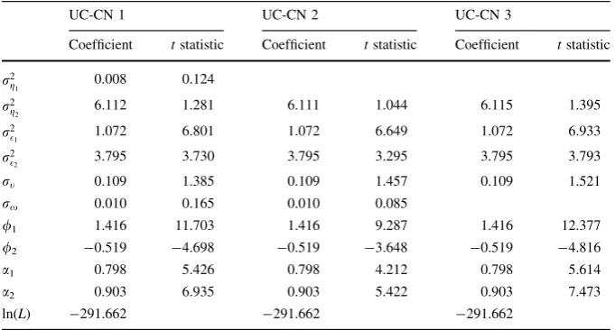
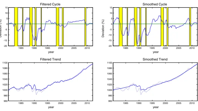
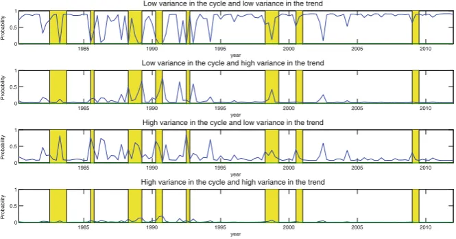
From this analysis, we opt for the UC-NC model1, which presents a mixture of normals in the disturbances of the trend and cyclical components of output. The thusly obtained trend clearly reflects the structural change that took place in the early 1990s. After a sharp decrease in the trend or potential GDP, a result of the severe adjustment measures that were carried out, GDP grew in a more stable fashion in the following years. In a similar way, an increase in the potential GDP growth rate can be observed from 2002 onwards, which coincides with the enactment of monetary reforms. Finally, the obtained cycles are congruent with the evolution of the Peruvian economy and with the recession periods that have been traditionally considered.
The remainder of this document is structured as follows. Section2 contains a review of the literature and the rationale behind the chosen method, Sect.3 describes the applied methodology and presents a brief analysis of the data, Sect.4 contains the results and Sect.5 presents the conclusions.
2 Literature review
A first approximation in cycle analysis was given by Burns and Mitchell (1946), who compiled the first timeline of business cycles for the United States. The cycle was defined as the expansion of several economic activities, followed by a recession and then a period of recovery. Several macroeconomic indicators were used and the simultaneous switch of signs was analyzed. A cycle was established for each indicator and an index was built for the whole economy’s cycles. Subsequently, NBER2applied this methodology for the classification of cycles.
The main disadvantage of this classification is the lack of measurement of the economic cycle and the delays in the identification of the recessionary cycles in a rapidly growing economy. Regarding the first point, Fellner (1956) estimates the business cycle as the residual between a series and its trend, where the trend is deterministic and is modeled as a polynomial that depends on time. As to the second point, Zarnowitz and Boschan (1977) provide a new approach, identifying ‘‘growth cycles’’ that have a lead with respect to the NBER chronology.
Beveridge and Nelson (1981) reject the imposition of a deterministic trend as the trend component of a series. They suggest that the trend component follows a stochastic process that may not necessarily be stationary. By means of a stationary ARIMA model in first differences, they estimate the trend component, while the cyclical component is estimated by residual. This procedure is applied to all macroeconomic indicators used by NBER for the classification of cycles. Each of the series is modeled as an ARIMA(p, 1,q) process, using the Box and Jenkins (1976) method for the identification of the parameters. Finally, a composite index is assembled by weighting the obtained cycles and then compare the results with the
1
UC-CN means unobserved components model with mixtures of normals in the disturbances of the cycle (C) of output, and of the trend level (N).
2 The National Bureau of Economics Research is the institution in charge of establishing the duration of
NBER chronology and that by Zarnowitz and Boschan (1977). Their results show a lead in the cycle periods and the same duration in the expansions and recessions. This is a contrast to NBER, which marks longer expansionary cycles and shorter recession periods.
Nelson and Plosser (1982) maintain the idea that output is led by a stochastic trend, and they analyze the principal yearly macroeconomic series of the United States from 1909 to 1970. They apply a unit root test (Dickey and Fuller1979; Said and Dickey1984), and conclude that the majority of the series, including GDP, do not reject the hypothesis of unit root. That is, the series are not stationary around a trend. Hence, the permanent or trend component follows a random walk, whereas the cyclical component follows a stationary behavior. In order to identify these components, they suggest a model of unobserved components, estimating the cycle through a signal extraction method (Friedman 1957; Muth 1960). Their results indicate that the real perturbations that affect the permanent component of output are the main sources of economic fluctuations. This idea was reinforced by Campbell and Mankiw (1987), who find persistence in the long term shocks on US GNP; according to these authors, an innovation of 1 % on real GNP is associated with an increase of more than 1 % in the long-term trend, and from that a negative correlation between the trend and cyclical components is drawn.
One feature of the decomposition by ARIMA models is that the identification of the trend and the cycle is only possible if a negative correlation between real innovations and the transitory cycle is assumed. Another form of decomposition involves the use of unobserved component models (UC), where identification implies a null correlation between the innovations of the cyclical and the trend components. From this perspective, Watson (1986) studies the annual series of GNP, available income and the consumption of non-durable goods in the United States from 1950 to 1985. GNP is modeled as an ARIMA(0, 1, 1), income as an ARIMA(0, 1, 4) and consumption as an ARIMA(0, 1, 0). Similarly, each series is modeled in non-observed components, where the trend is a random walk with drift, the cycle is an AR(p=q?1) stationary process, and the perturbations between both components are not correlated. Watson (1986) finds that in the unobserved components model, innovations have a lower impact on output fluctuations. However, this model is not significantly better than the ARIMA model. From this, he concludes that the sole specification of the model has consequences in the determination of cycles and hence, in economic policy decisions.
In a similar way, Clark (1987) applies a model of unobserved components with quarterly information for GDP and the industrial production of the United States from 1947 to 1985. He retains the assumption of non-correlation between errors, but modifies the behavior of the trend, whose slope is now assumed to follow a random walk. At the same time, the cyclical component follows an AR (2) process for both series. From this specification, he concludes that the fluctuations in output depend almost in 50% of innovations in the cyclical component.
component filter and the smoothing require large amounts of computational resources.
Stock and Watson (1988) summarize the main findings in the decomposition of output on the basis of ARIMA models or unobserved components. A distinct difference between both models is the importance of real innovations in the former and to a lesser degree in the latter. They argue that this is due to the presence of a stochastic trend and the hereby derived specification. On the one hand, the perfect correlation in ARIMA models is originated because in them, both the trend and the cyclical component are subject to only one type of shock. In this case, the correlation tends to be negative and allows one to define the cycle as an adjustment process in economic growth caused by a real shock, although the opposite is difficult to justify. Whereas, the null correlation between the cycle and trend lead to a higher relevance of the cyclical component. In both cases, identification defines in a certain way the preponderance of the one or the other types of shocks; however, there remain obstacles in the identification of the real source of the shock. On the other hand, the authors conclude that the assumption of the existence of a stochastic trend in the main macroeconomic series is valid and resembles the behavior of the United States data. Additionally, they conclude that in general, the permanent component has a higher impact on the economic fluctuations of that country.
In contrast, Cochrane (1988) puts in discussion the presence of a unit root in the GNP series of the United States. He concludes that in any case, its presence is minor and thus the shocks on the trend component are less important. On the other hand, Perron (1989) rejects the existence of a unit root for several of the series, including GNP, previously analyzed by Nelson and Plosser (1982). He posits as alternative hypothesis that the data generating process is stationary with a broken trend. The novelty in his proposal is the inclusion of two exogenous shocks that have a permanent effect on output. The first, due to the 1929 crisis, prompts a change in the trend level of GNP; the second, due to the oil crisis of 1973, brings about a change in the slope of the trend, which can be interpreted as the growth rate of potential GNP. The author concludes that the economic fluctuations are stationary around a broken deterministic trend. In consequence, changes in transitory behavior have a higher weight on business cycles.
The multivariate model of Blanchard and Quah (1989) presents a variant to the ARIMA and unobserved components models. They suggest a structural VAR model for quarterly output and unemployment in the United States from 1950 to 1987. They solve the identification problem of univariate models by assuming that shocks of unemployment or demand do not have a permanent impact on output. On that basis, the authors find that demand shocks are relevant in the short and medium term, whereas supply shocks have a permanent impact on output and accumulate over time.
An important feature of the previously described models is that they assume linearity in the series and symmetry in the disturbances. However, the empirical evidence shows that negative shocks have a short duration and have a more profound impact on the output level. Friedman (1964) called this empirical peculiarity the ‘‘plucking’’ effect. The length of a recession is correlated to the length of the subsequent expansion, but not the opposite; that is, there is an asymmetry between positive and negative shocks. Besides, the drop of output varies in intensity, but always returns to the potential level. Friedman (1993) analyzes the output of the United States from 1975 to 1990 and finds evidence in favor of the ‘‘plucking’’ effect.
In a similar way, Neftci (1984) finds that in unemployment cycles in the United States, the transition from a recession to an expansion takes place without drastic changes; that is, there are asymmetries in the unemployment cycles. This effect is known in the business cycle literature as ‘‘duration dependence’’. A positive dependence on duration would indicate that expansions or recessions are more likely to end when they mature over time. Sichel (1991), Diebold and Rudebusch (1990), and Diebold et al. (1993) find evidence in favor of duration dependence in the GNP series of the United States, Great Britain and France. However, in all cases the dependence is asymmetrical, that is, it occurs only in recessions or in expansions. Sichel (1993) finds asymmetry in the depth of the unemployment cycle, industrial production and United States’ GNP. That is, during recessions, output drops below trend more than it rises during expansions.
Taking into consideration the evidence of non-linearity of the series, Hamilton (1989) proposes a non-linear model with regime changes. In that model there are two regimes, one of positive output growth and one of negative growth. According to the author, the output in differences depends not only on its lags, but there is also a discrete change in the mean that generates a transition between positive and negative growth regimes. The change in the mean is caused by an unobserved exogenous variable that follows a first-order Markov process. One of the advantages of the model is the estimation of regime changes from data in the series. Additionally, it is possible to estimate the probabilities of being in a given regime, for example, a recession. Hamilton (1989) employs an AR (4) specification in order to model the quarterly growth rate of US GNP from 1950 to 1985. He finds a recurrence in the regime changes. The transition from expansion to recession is associated with a drop of 3 % of real output and a similar drop in the permanent component; that is, permanent shocks dominate output fluctuations. Later, Krolzig (1997) carries out a characterization of the different variables of the Markov-switching model, with changes in the mean, variance and/or intercept. Additionally, he generalizes Hamilton’s proposal to a multivariate analysis. Whereas, Goodwin (1993) applies the Hamilton model to 8 countries of OECD without finding significant gains in comparison to other linear models, although the symmetry hypothesis is rejected for the majority of the countries.
This latter model considers the existence of two regimes and the change between them follows a transition function that can be modeled with a logistic or exponential distribution. This function depends on an observable transition variable and is increasing when approaching or surpassing a given threshold. From this starting point, a smoothed transition between regimes is generated. It is important to note that a previous step to the application of the model is to reject the non-linearity of the series, the alternative hypothesis being the logistic or exponential STAR model. Following these criteria, Tera¨svirta and Anderson (1992) estimate the STAR model for the quarterly production index or 13 OECD economies. They find that the model is adequate in describing the non-linearities and asymmetries of the series.
In the area of multivariate models, Kuttner (1994) exploits the theoretical relation between output and inflation through the Phillips curve. He proposes a bivariate decomposition of unobserved components. Output is decomposed in trend and cycle in a similar way as in the Clark (1987) model, whereas inflation depends on past inflation and the deviation of output from its potential level. One of the advantages of this method resides in the possibility of incorporating in a simple way the theoretical relations between output and other economic variables. In his analysis, Kuttner (1994) finds that the coefficient that measures the sensitivity between the output gap and inflation is significant; that is, the Phillips curve is relevant in the analysis of both series. Besides, the permanent shocks have larger impacts on output, in comparison to a univariate model.
Taking into consideration the evidence of asymmetry in cycles, Kim and Nelson (1999a) specify a model of unobserved components denominated ‘‘plucking’’. In this model, the cyclical component follows an AR (2) process, with disturbances composed by a mix of two types of shocks: symmetrical and asymmetrical. The existence of the latter depends on the probability of occurrence of a recession; that is, in normal times only the symmetrical shock remains. The trend component is modeled as a random walk that suffers two types of disturbances: one on the level and another that affects the trend rate of growth. The authors follow Friedman (1993) in specifying the output trend as a ‘‘ceiling’’ trend; according to this, output reaches a maximum level in normal times and deviates below trend during recessions. The model is applied to quarterly GNP series and the unemployment rate in the United States for the 1951:1995 period, generating negative cycles during the recession periods. In consequence, in normal times output is driven by permanent shocks; real business cycle models are thus ideal in explaining the behavior of output. However, in times of recession the transitory shocks predominate, and monetary and other demand-oriented models are pertinent. A later application of the ‘‘plucking’’ model is carried out by Mills and Wang (2002) for the G7 countries.
‘‘band-pass’’ that eliminate the high and low frequency components, allowing the extraction of smoothed cycles. One of the advantages of these filters is their ease of application, since they do not assume a given behavior of the series. However, they present some disadvantages. In the first place, ‘‘high-pass’’ filters such as Hodrick and Prescott (1997) can generate spurious cycles (Harvey and Jaeger 1993). For their part, ‘‘band-pass’’ filters do not completely isolate the cycle, which could be confused with the trend in differences (Murray 2003). A generalization of the previous filters are the ‘‘Butterworth’’ filters proposed by Harvey and Trimbur (2003), from which data-consistent high-pass or band-pass filters can be obtained. However, despite the improvements in filter specification, the problem of symmetry in the cycles and a lack of theoretical fundamentals in their construction remains.
Regarding the assessment of these methods, Canova (1998) carries out a balance on the application of different filters to quarterly macroeconomic series such as output, consumption, investment, and productivity in the United States for the 1953–1986 period. His purpose is to contrast empirical regularities with the proposed economic theory, regardless of the utilized filter. Among the main stylized facts he finds with a certain robustness are a high correlation between the output cycles and investment, and a lower volatility of consumption with respect to output, although with differences in magnitude given the used filter. In contrast, the procyclicality of productivity depends on the utilized filters. Other stylized facts of modern macroeconomics are: the negative correlation between output cycles and unemployment, and the negative, short term relation between inflation and unemployment cycles. Starting from this stylized facts, several authors build models of multivariate unobserved components in order to obtain in a joint manner the cycles and trends of different series. For example, Apel and Jansson (1998) estimate the output and unemployment cycle in the United States, Canada and the United Kingdom by using Okun’s law. Laubach (2001) estimates NAIRU and the employment cycles for the G7 countries using the Phillips curve. And Dome´nech and Go´mez (2006) include an investment behavior equation that depends on the output cycle, in addition to Okun’s Law and the Phillips Curve.
cycles thus obtained are symmetrical. Later, Oh and Zivot (2006) extend the proposal of Morley et al. (2003) applied to the Clark (1987) model, which in a reduced form is an ARIMA (2,2,3), and reject the idea of a trend with double drift. Similarly, Basistha (2007) extends the model to a multivariate analysis.
In the domestic literature, there is the work of Cabredo and Valdivia (1999), who apply diverse methods for estimating Peruvian potential output from 1950 to 1997 starting from an aggregate production function, the Hodrick and Prescott (1997) filter, and a structural VAR. On the other hand, Miller (2003) distinguishes among methods of the structural and non-structural kind. For the former, he employs the Hodrick and Prescott (1997) filter, a method of segmented trend, a non-parametric smoothing method, the Baxter and King (1999) filter, and the Beveridge and Nelson (1981) decomposition; whereas, for the latter, he employs the production function and a structural VAR. Her estimations are based on the yearly Peruvian GDP series from 1951 to 2001, and she finds that all methods have the ability to identify the cycles in the economy, although they differ in the magnitude of the cycle and tend to underestimate the recessionary cycles during the big recessions of the 1980s.
In analogous fashion, Seminario et al. (2007) use a set of methods such as the Hodrick and Prescott (1997) filter, the Baxter and King (1999) filter, the peaks method3, the method of Marfa´n and Artiagoitia (1989) and a sectoral method in order to obtain potential output from 1950 to 2007. On the other hand, Castillo et al. (2007) use the Baxter and King (1999) filter in order to obtain the cyclical component of output within the analysis of the stylized facts of the Peruvian economy.
From another viewpoint, Rodrı´guez (2010a) uses three non-linear methods in order to decompose the cyclical element from a series. The STAR model by Tera¨svirta (1994), the ‘‘Markov switching’’ of Hamilton (1989) and the ‘‘plucking’’ model of Kim and Nelson (1999a) are applied to the analysis of the quarterly series of Peruvian GDP from 1980 to 2005. The three models reject the linearity of the series. The MSIAH (3) model, which is based on a Markov switching model with three regimes and an AR (4) from the output in differences, generates recession periods that are more in line with the empirical dating of recessions4. However, periods following 1990 and characterized as recessions (1998, 2011) are not captured by any model. The explanation proposed by the author is based on the strong contractions or expansions of the Peruvian economy, which makes the correct identification of cycles more difficult.
In Rodrı´guez (2010b), the estimation of the cyclical component of GDP is supported by the neo-Keynesian theory. Keeping the specification of Basistha and Nelson (2007), one assumes the existence of a Phillips curve that depends on the expected inflation, past inflation and the output cycle. A bivariate model of unobserved components allows one to extract the output cycle for the period 1980–2005. In a similar way, the relevance of the Phillips curve is tested.
3
Methodology that was proposed to NBER in order to identify the peaks of a series. The authors follow the explanation provided by Ochoa and Llado´ (2003) with respect to this method.
4 A recession is defined as a period which registers falls in real GDP for more than two consecutive
Additionally, in comparison to other models, significant differences are obtained with the exception of the Clark (1987) model.
While keeping the multivariate specification, Rodrı´guez (2010c), following Do´menech and Go´mez (2006), uses an unobserved components model in order to capture the relations between output trend and cycle, the Phillips curve, Okun’s Law and an investment behavior function. Using this model, he extracts the cyclical component of output, the underlying inflation rate and the structural or NAIRU unemployment rate from 1980 to 2007.
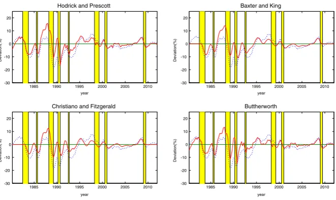
Recently, Wada and Perron (2006) and Perron and Wada (2009) have suggested a new model of decomposition of trend and cycle, which admits structural changes in the trend and asymmetry in the cyclical component. They use a non-linear model of unobserved components, whose disturbances consist of a mixture of normal distributions both for the cyclical component and the trend component. This specification allows one to capture swift changes in an endogenous way, at the same time that it overcomes the discussion between ARIMA and unobserved component models, since it does not impose restrictions on the correlation between cycle and trend disturbances. After analyzing quarterly GDP of the United States for the 1947-1998 period, the authors find that, with the exception of changes in the slope, the trend of output is deterministic. On the other hand, the cyclical component presents asymmetries and is relevant in economic fluctuations. Besides, in comparison to other methods (Hodrick and Prescot1997; Baxter and King1999; Beveridge and Nelson1981; unobserved components), the cycles of boom and recession are better adjusted to the NBER timeline.
The Wada and Perron (2006) and Perron and Wada (2009) methods present certain advantages with respect to earlier models, especially when dealing with series that have undergone structural changes. In the first place, the method features a great degree of flexibility to capture the different changes in the behavior of the series. A structural change can be modeled as an abrupt shock to trend that takes place with a low probability, whereas smaller shocks occur with a higher probability, giving shape to a stochastic trend. In the same way, low and high impact shocks on the cycle can reflect short term policies that are very expansionary in situations of crisis, but less so in normal times.
Secondly, this method overcomes the identification problem that is present in both ARIMA and unobserved components models, for each disturbance consists of a mixture of two normal distributions, which are not correlated with other disturbances (although, as a whole, the mix can be correlated with another one). This specification is an alternative to that proposed by Morley et al. (2003), with the advantage that it admits asymmetries in the output cycles.
of Kim and Nelson (1999a) do not identify recessionary periods after 1990. One plausible explanation to the latter is that these models assume the existence of a Markov process, which is not very useful for Peruvian GDP that shows a very different behavior in the periods before and after 1990.5
Fourthly, the specification to be used allows the identification of break points in an endogenous fashion, and finally, it is superior to statistical high-pass or band-pass filters, as it does not impose smoothing restrictions to the series.
In view of these advantages, it is convenient to apply the Wada and Perron (2006) and Perron and Wada (2009) method to decompose Peruvian GDP into trend and cycle. First, we attempt to capture the effect of non-linearities and asymmetries present in output that have been documented by Rodrı´guez (2010a). And, second, to identify the structural change that took place in the early 1990s, where important institutional reforms were enacted that, according to Castillo et al. (2007), made possible a more stable growth of the economy. It is important to highlight that previous estimations could not associate that structural break with a behavior of the trend or a long-term component of output. Finally, we expect that this methodology will allow a better identification of recessive cycles, especially in periods after 1990, which is why the obtained cycles will be compared with those produced by other methods and with the timeline of recessions that is usually employed.
3 Methodology
We aim to extract the trend and cycle of Peruvian GDP by using the method proposed by Wada and Perron (2006). In consequence, we built an empirical model of non-linear output decomposition into non-observable components, according to the following specification:
yt¼stþctþxt; ð1Þ
st¼st1þbtþgt; ð2Þ
bt¼bt1þtt; ð3Þ
ct¼/1ct1þ/2ct2þt; ð4Þ
whereytis the observable series,stis the trend,ctis the cyclical component,btis the
variable that allows changes in the trend slope andxt;gt;tt; t are the disturbance
terms. The model is non-linear due to the behavior of the disturbance terms. If they are represented byut, then they have the following distribution:
ut¼ktc1tþ ð1ktÞc2t; ð5Þ
5 In the early 1990s, a large structural adjustment was applied to the economy and institutional reforms
whereciti.i.d.N 0;r2i
andkti.i.d. BernoulliðaÞ.6The error int behaves as a
Nð0;r2
1Þwith probabilitya and asNð0;r 2
2Þwith probability ð1aÞ. This
specifi-cation allows us to capture the non-linearities of the path of the output. For example, ifatakes a value close to 1 andr22is much higher thanr12, then there would be, most
of the time, periods of low variance or ‘‘normal’’, whereas on an exceptional basis, large shocks that alter the level of the series would take place. The latter would be ‘‘atypical’’ periods that could be associated with periods of recession or structural changes.
Several feasible scenarios can be considered. In one of them, the disturbance
xtwould be expected to be very small or close to zero in ‘‘normal periods’’ and of
a larger magnitude only in the case of atypical situations, where the output level is affected but not the potential level, for example, during natural disasters. In another scenario, the disturbance gt generates a stochastic trend or, on the
opposite, ifr12=0, a deterministic trend with occasional changes in the level.
With respect to the disturbancett, one could expect it to be small most of the time
and to take a larger magnitude only in atypical periods. Finally, the disturbancet
can have different variances depending on whether the economy is in a period of moderate growth or high volatility. Each of these scenarios is not independent of the other and they can combine indistinctly, thereby affecting the evolution of economic cycles.
Wada and Perron (2006) focus on the importance of changes in the level and slope of the trend, and as such, their model only allows the disturbancesgtandttto
be composed by a mixture of normals. In contrast, Perron and Wada (2009) allow a change in the slope of the trend and asymmetrical cycles thanks to the specification ofttandt as mixtures of normals.
In the last 30 years, Peruvian GDP has undergone important changes, ranging from deep losses and periods of fast growth, to drastic changes in the production structure. This supports the hypothesis that the aggregate output has a non-linear behavior that includes discrete changes in its trend or its potential growth rate. These changes can be originated by positive or negative disturbances that take place with a small probability, but have a large impact on the dynamic of output in the long term, for example, periods of economic reforms, internal conflict or institutional reform. On the other hand, during recessions, the magnitude of the variation of output tends to be larger than during expansion periods, but the duration of this high variance period is relatively short. This can be explained by an asymmetrical cyclical component where disturbances of large magnitude, which take place infrequently, have a serious impact on output in the short term, for example, in the event of adverse external shocks and monetary or fiscal policies.
Regarding empirical studies, Rodrı´guez (2010a) finds evidence in favor of the presence of non-linearities in Peruvian GDP and of asymmetries in its cyclical component. In consequence, one could establish the existence of mixtures of normals in the trend level, in its growth rate, and in the cyclical component of
6 In a Bernoulli distribution (a) the random variable takes the value of 1 if the event occurs with success
output. One could even allow the presence of a mixture of normals in the measurement equation that would capture the effect of atypical output changes or outliers. For example, natural disasters that drastically affect the level of Peruvian output, and take place irregularly, would be mistakenly estimated within the cyclical component. However, according to Wada and Perron (2006), the inclusion of all disturbances as mixtures of normals implies an unstable estimation algorithm.
Given the previous discussion, we considered to restrict the number of scenarios under consideration. Wada and Perron (2006) utilize up to two disturbances with mixtures of normals. This restriction in the number of mixtures is a consequence of a problem of identification. For example, a country that does not undergo structural changes during the period of analysis would have a very stable trend and periods of high and low variance would not be justified. The imposition of both regimes could generate extreme values in the variances and their probabilities of occurrence. In the case of Peru, the opposite is true: the fluctuations of output are very irregular and one could even estimate a model with three mixtures of variables.
We take on all estimation possibilities starting with the simpler models that admit only one mixture of normals. We then continue with models that contemplate combinations of two mixtures of normals, and explore the possibility of a model that admits up to three mixtures of normals, in order to find the best specification for the Peruvian economy. As such, the following estimations are laid out:
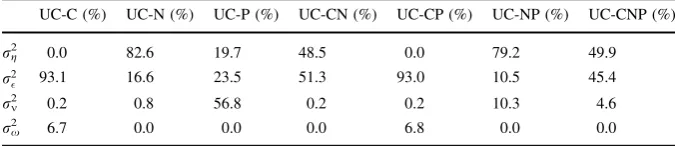
• UC-C: a model with a mixture in the cyclical component (t).
• UC-N: a model with a mixture in the disturbances of the trend level (gt). • UC-P: a model with a mixture in the disturbances of the trend slope (tt). • UC-CN: a model with mixtures in the disturbances of the cyclical component
and the trend level (t;gt).
• UC-CP: a model with mixtures in the disturbances of the cyclical component and the trend slope (t;tt).
• UC-NP: a model with mixtures in the disturbances of the trend level and trend slope (gt,tt).
• UC CNP: a model with mixtures in the disturbances of the cyclical component, the trend level and the trend slope (t;gt;tt;).
3.1 Estimation method
The estimation of the non-observable components will be carried out by a state-space representation. For notation purposes, it is important to have in mind thatgt,tt
and t are the disturbances on the trend level, the trend slope and the cyclical
component, respectively. Some or all of which consist of a mixture of normal distributions, depending on the model; whereas the remaining disturbances follow a normal distribution. Moreover,aiis the probability that the disturbancei¼gt; t;tt
the high variance regimeri22. The estimation method starts from the following
state-space representation:
yt¼Hxtþxt
xt¼Fxt1þGut;
ð6Þ
where
H0¼
1 1 0 0 2 6 6 4 3 7 7 5; xt¼
st
ct
ct1
bt 2 6 6 4 3 7 7
5; F¼
1 0 0 1
0 /1 /2 0
0 1 0 0
0 0 0 1
2 6 6 4 3 7 7
5; G¼I; ut¼
gt t 0 tt 2 6 6 4 3 7 7 5
ð7Þ
In contrast to conventional models, the disturbance vectorutdoes not follow a
normal distribution. However, it is feasible to assign a normal distribution with possible states to the state-space representation. The variance and covariance matrix of ut takes M possible states that are generated as a result of the
combination of values taken by the Bernoulli random variables. For example, in a model with a mixture of normals there are only two possible states that are associated with periods of low and high variance, whereas in a model with two mixtures of normals, four possible states will exist associated with combinations of high and low variance for each disturbance. In consequence, there are 2m possible states, wheremis the number of disturbances with mixtures of normals. The Q variance and covariance matrix for a model with only one mixture of normals such as UC-C7 is given by:
Q¼
r2
g 0 0 0
0 r2
1 0 0
0 0 0 0
0 0 0 r2
t 2 6 6 4 3 7 7 5 r2
g 0 0 0
0 r2
2 0 0
0 0 0 0
0 0 0 r2
t 2 6 6 4 3 7 7 5 8 > > < > > : 9 > > = > > ; ;
where each state or regime occurs with probabilitiesa1andð1a1Þ. TheQmatrix
for a model with two mixtures of variables like UC-CN would be:
Q¼
r2
g1 0 0 0
0 r2 1 0 0
0 0 0 0
0 0 0 r2
t 2 6 6 4 3 7 7 5 r2
g2 0 0 0
0 r2 1 0 0
0 0 0 0
0 0 0 r2
t 2 6 6 4 3 7 7 5 r2
g1 0 0 0
0 r2 2 0 0
0 0 0 0
0 0 0 r2
t 2 6 6 4 3 7 7 5 r2
g2 0 0 0
0 r2 2 0 0
0 0 0 0
0 0 0 r2
t 2 6 6 4 3 7 7 5 8 > > < > > : 9 > > = > > ; ;
where each state occurs with probabilities a1a2;a1ð1a2Þ;ð1a1Þa2, and ð1
a1Þð1a2Þrespectively. Finally, theQvariance and covariance matrix for a model
with 3 mixtures of normals would be defined as:
7
Q¼
r2
g1 0 0 0
0 r2 1 0 0
0 0 0 0
0 0 0 r2
t1 2 6 6 6 6 4 3 7 7 7 7 5 r2
g1 0 0 0
0 r2 1 0 0
0 0 0 0
0 0 0 r2
t2 2 6 6 6 6 4 3 7 7 7 7 5 r2
g2 0 0 0
0 r2 1 0 0
0 0 0 0
0 0 0 r2
t1 2 6 6 6 6 4 3 7 7 7 7 5 r2
g2 0 0 0
0 r2 1 0 0
0 0 0 0
0 0 0 r2
t2 2 6 6 6 6 4 3 7 7 7 7 5 r2
g1 0 0 0
0 r2 2 0 0
0 0 0 0
0 0 0 r2
t1 2 6 6 6 6 4 3 7 7 7 7 5 r2
g1 0 0 0
0 r2 2 0 0
0 0 0 0
0 0 0 r2
t2 2 6 6 6 6 4 3 7 7 7 7 5 r2
g2 0 0 0
0 r2 2 0 0
0 0 0 0
0 0 0 r2
t1 2 6 6 6 6 4 3 7 7 7 7 5 r2
g2 0 0 0
0 r2 2 0 0
0 0 0 0
0 0 0 r2
t2 2 6 6 6 6 4 3 7 7 7 7 5 8 > > > > > > > > > > > > > > < > > > > > > > > > > > > > > : 9 > > > > > > > > > > > > > > = > > > > > > > > > > > > > > ; ;
where each state occurs with probabilitiesa1a2a3;a1a2ð1a3Þ;a1ð1a2Þa3;a1ð1
a2Þð1a3Þ;ð1a1Þa2a3;ð1a1Þa2ð1a3Þ;ð1a1Þð1a2Þa3 and ð1a1Þð1
a2Þð1a3Þrespectively.
The estimation process starts with the application of the Kalman filter, which follows the same principles as the state-space model with normal disturbances laid out by Harvey (1989). Afterwards, the Hamilton filter is added according to the approach of Kim and Nelson (1999b). The Kalman filter considers the estimation of the expected value of thext vector, conditional to the information available until
periodt. This new vectorxt|tis called filtered estimator. In a second stage, we built an
estimator conditional to all information available in the sample, vectorxt|T, which is
called smoothed estimator and is obtained after utilizing a smoothing algorithm. This last vector is relevant for the study, for the aim is to carry out an inference of the non-observable componentsðst;ctÞfrom the basis of all information available. The steps
of that estimation are described as follows.
Step 1: Kalman FilterWe look for the best estimator of the state vector and its
variance and covariance matrix. To this end, we know that in a model with normal disturbances, the best linear estimator of the state vector is the linear minimum mean square error estimator (MMSE),xt|t-1, which is forecast on the basis of all
information available up to the periodt-1. For its part,Pt|t-1is the mean square
error (MSE) or the variance of the forecast error ofxt|t-1. Formally:
xtjt1¼E½xtjYt1; ð8Þ
Ptjt1¼E½ðxtxtjt1Þðxtxtjt1Þ0jYt1: ð9Þ
However, there are high and low variance regimes that are represented in the different states taken by the Q variance and covariance matrix. Hence, if we denominateStas the variable that indicates the regime (low or high volatility) in
which the state vector is located in timet, we obtain:
xijtjt1¼E½xtjYt1;St1¼i;St¼j i;j¼1;. . .;M ð10Þ
Pijtjt1 ¼E ðxtxtjt1Þðxtxtjt1Þ0jYt1;St1¼i;St¼j
; ð11Þ
number of possible states. This representation is similar to the Markov Switching model by Hamilton (1989). The fundamental difference is that the probability of being in the regimeStdoes not depend on the past probability of being in the regime
St-1, which only affects the state variables. In a simple example, one could assert
that if int-1 the probability of being in a high volatility period was very low, this does not imply that intthe volatile period takes place. Conditional toSt-1=iand
St=j, the following algorithm of the Kalman filter is obtained:
xijtjt1¼Fxti1jt1; ð12Þ
Pijtjt1¼FPit1jt1F0þGQjG0; ð13Þ
vijtjt1¼ytHxijtjt1; ð14Þ
ftijjt1¼HPijtjt1H0þR; ð15Þ
xijtjt¼xijtjt1þPtijjt1H0hftijjt1i
1
vijtjt1; ð16Þ
Pijtjt¼ IPijtjt1H0hftijjt1i
1
H
Pijtjt1; ð17Þ
wherexti-1|t-1is the value thatxt-1is inferred to take on the basis of information
available up to t-1 and conditional to being in the state St-1=i; xtij|t-1 is the
inference ofxtuntilt -1 givenSt-1=iandSt=j. On the other hand,Ptij|t-1is the
mean square error ofxtij|t-1conditional toSt-1=iandSt=j,vtij|t-1is the forecast
error of yt based on the information available until t-1 and conditional to
St-1=i and St =j ; ft|t-1
ij
is the conditional variance of the forecast errorvt|t-1
ij
. Finally, xtij|tand Ptij|tare the values that the variables are inferred to take after the
updating process of the Kalman filter takes place.
Step 2: Hamilton FilterWe aim to infer the probability associated with the state
vector estimator and its variance and covariance matrix.
At the start of the iteration process, for the periodt, givenSt-1=iandSt=jand
taking into consideration that both variables are independent8, we can calculate the joint probabilities of being in a given regimeStand to originate from another St-1
regime, conditional to the past realizationsYt-1in the following way:
PrðSt1¼i;St¼jjYt1Þ ¼PrðSt¼jjSt1¼iÞPrðSt1¼ijYt1Þ;
PrðSt1¼i;St¼jjYt1Þ ¼PrðSt¼jÞPrðSt1¼ijYt1Þ:
ð18Þ
Besides, we have the joint density function ofyt,St-1andSt:
pðyt;St1¼i;St¼jjYt1Þ ¼pðytjSt1 ¼i;St¼j;Yt1ÞPrðSt1¼i;St¼jjYt1Þ;
ð19Þ
where the marginal density function ofytis given by:
8 In contrast with the model of Hamilton (1989), where Pr
ðSt1¼i;St¼jÞ is the probability of
pðytjYt1Þ ¼ XM
j¼1 XM
i¼1
pðytjSt1;St;Yt1ÞPrðSt1 ¼i;St ¼jjYt1Þ; ð20Þ
and the conditional density functionpðytjSt1;St;Yt1Þis calculated on the basis of
the forecast error and its variance, which are obtained from the equations of the Kalman filter:
pðytjSt1;St;Yt1Þ ¼
1
ffiffiffiffiffiffi
2p
p ftijjt1 1=2
exp
vtijj0t1ftijjt1
1
vijtjt1
2 8 > < > : 9 > = >
;: ð21Þ
WhenYtis observed in periodt, it is possible to update the probability PrðSt1¼
i;St¼jjYt1Þas follows:
PrðSt¼jÞPrðSt1¼ijYtÞ ¼PrðSt1¼i;St¼jjyt;Yt1Þ ¼
pðyt;St;St1jYt1Þ
pðytjYt1Þ
;
PrðSt1¼i;St¼jjYtÞ ¼
pðytjSt;St1;Yt1ÞPrðSt1 ¼i;St¼jjYt1Þ
pðytjYt1Þ
;
ð22Þ
and to obtain the probability associated with each regime St conditional to the
information available until periodt:
PrðSt¼j;YtÞ ¼ XM
i¼1
PrðSt1¼i;St¼jjYtÞ: ð23Þ
Finally, being YT ¼ ðy1;y2;. . .;ytÞ the vector of data available in period t, the
likelihood function is maximized:
ln½pðYTÞ ¼ln XT
t¼1
pðytjYt1Þ
" #
: ð24Þ
Step 3: CollapsingThere is a dimensionality problem if one aims to estimate the
previously described algorithm, since it requires the estimation of 4testimators and their respective mean squared errors. In order to render the Kalman filter operable, a process of ‘‘collapsing’’ is employed, which re-approximates the estimatorsxtij|tand
Pijt|tin each periodttoxjt|tandPtj|t. Following Wada and Perron (2006), we adopt the
method of Harrison and Stevens (1976), where:
xtjjt¼
PM
i¼1PrðSt1¼i;St¼jjYtÞx ij tjt
PrðSt¼jjYtÞ
; ð25Þ
Ptjjt¼
PM
i¼1PrðSt1 ¼i;St¼jjYtÞ P ij tjtþ x
i tjtx
ij tjt
xi
tjtx ij tjt
0
n o
PrðSt¼jjYtÞ
: ð26Þ
The first equation indicates that in each periodMvectors of statextij|tare generated,
St-1 and of being in another regime St. One proceeds in similar fashion for the
MvariancesPtij|tthat are generated in each period. Since the state variable is
con-ditional only to being in the regimeSt=j, the estimator filtered in each periodtis
obtained as follows:
xtjt ¼
XM
j¼1
PrðSt¼jjYtÞxtjjt: ð27Þ
The collapsing allows one to reduce the possible states that the variables can take. For example, if one starts int=1 there arejpossible states, int=2 each of them generatesj additional possible states, and so on; in time, the dimension of states grows. With the proposed method, in each period t there will only be j possible states that are of interest for the analysis of cycles; that is, those linked to periods of high and low variance.
3.2 Initial values
The recursive method of the Kalman filter requires initial values for the state vector
x0|0and for the variance of the forecast errorP0|0. These values are chosen after the
proposal of Wada and Perron (2006). For example, in the case of the state vector, we have:
x0j0 ¼½s0;0;0;b0
0 ;
where the initial trend value,s0, is the first observation of GDP. The initial value of
the slope,b0, corresponds to the simple average of the growth rate of the first four
quarters.9Whereas, the initial values of the cycles,ctandct-1, are their steady state
values. On the other hand, the initial values of the variance of the forecast error are given by:
P0j0¼
1eþ08 0 0
0 P 0
0 0 1eþ08
2 4
3 5;
where the submatrixPis obtained from vecðPÞ ¼½I2F1F1
1
vecðQ1Þ;with
F1¼ /1 /2
1 0
Q1¼ r
2 1 0
0 r2 2
SubmatrixPrepresents the inconditional variance of the cyclical component and is estimated assuming the stationarity of that component. Since the trend and its slope are not stationary, it is not possible to estimate their variances in the same way. One alternative is to follow the proposal of Harvey and Phillips (1979), which considers extremely large numbers, with which the variance and covariance matrix approa-ches its exact value after several iterations. It is important to highlight that the state variables (trend and cycle) are not sensitive to these specifications.
9 Wada and Perron (2006) take as initial value of the slope the first rate of growth of the series. However,
3.3 Restrictions and initial conditions
The proposed model, and in general the models with mixture of gaussian errors, present a parameter identification problem. The likelihood function remains constant given a permutation of their individual components, and the estimation parameters cannot be obtained. This problem is known as ‘‘label switching’’ and is analyzed by Hamilton et al. (2004). In the specific case ofp(yt|Yt-1) we obtain that:
p yð tjst1;st;Yt1ÞPrðst1¼i;st¼jjYt1Þ
þp yð tjst1;st;Yt1ÞPrðst1 ¼i;st¼jjYt1Þ
¼p yð tjst1;st;Yt1ÞPrðst1¼i;st¼jjYt1Þ
þp yð tjst1;st;Yt1ÞPrðst1 ¼i;st¼jjYt1Þ:
ð28Þ
In consequence, it is not possible to identify the statesiandi without carrying out a normalization. Wada and Perron (2006) impose restrictions in the parameters of the distributions with mixture of normals. And the restrictions vary for each of the G7 countries under analysis. For example, in the case of the United States, they assign a minimum probabilityða2¼0:9Þto the fact that the slope disturbances are
in the low variance regime and that the maximum value of such variance is
r2
t1 ¼0:01. We consider that for the Peruvian case, such values are very restrictive. We only impose as a restriction that the variances associated with the high volatility regime be higher than those associated with the low volatility regime, whereas the probability of being in the low volatility regime be at least 0.5. More than a restriction, this represents a normalization of the parameters that does not affect the decomposition into trend and cycle.
3.4 Smoothing
The estimation process is completed with the inference on the state vectorxtand on
the probabilities associated with each regime st, taking into consideration all
available information. That is, we aim to estimate Pr½st ¼jjYTyxtjTð1;2;. . .;TÞ. To
this end, the smoothing algorithm developed by Kim and Nelson (1999b) is employed. The main steps are described as follows.
The first step in the smoothing process is to backwards estimate the state vector and its variance for each periodt=T -1,T -2,…, 1 on the basis of estimated values in the filtering process, according to the following algorithm:
xjktjT¼xtjjtþPejkt xtkþ1jTxjktþ1jt; ð29Þ
PjktjT ¼PtjjtþPejkt Pktþ1jTPjktþ1jtePjkt0; ð30Þ
wherePejkt ¼P j tjtF
0 Pjk tþ1jT
h i1
, whereasxtjk|TandPtjk|Tare the values taken by the state
In the second step, the probabilities associated with each regime are estimated. Here, the following derivation of the joint probability of St =j and St?1=k is
made, conditional to the availability of all information:
PrðSt¼j;Stþ1¼kjYTÞ ¼PrðStþ1¼kjYTÞPrðSt¼jjStþ1¼k;YTÞ
PrðStþ1¼kjYTÞPrðSt¼jjStþ1¼k;YtÞ
¼PrðStþ1¼kjYTÞPrðSt¼j;Stþ1¼kjYtÞ
PrðStþ1¼kjYtÞ
;
ð31Þ
and
PrðSt¼j;YTÞ ¼ XM
k¼1
PrðSt¼j;Stþ1 ¼kjYTÞ: ð32Þ
Since each state variable depends on its regime,M9Mestimators ofxtjk|Tand ofPtjk|T
are generated, so that a collapsing process similar to the one previously described is undertaken, where:
xtjjT ¼
PM
k¼1PrðSt¼j;Stþ1 ¼kjYTÞxijtjT
PrðSt¼jjYTÞ
; ð33Þ
PtjjT ¼
PM
k¼1PrðSt¼j;Stþ1¼kjYTÞ PjktjTþ xtjjTxiktjT
xtjjTxik
tjT
0
n o
PrðSt ¼jjYtÞ
: ð34Þ
Finally, the smoothed state vector xt|T is built as the weighted average of the
Mvectorsxtj|T, given their respective probabilities:
xtjT ¼
XM
j¼1
PrðSt¼jjYTÞx j
tjT: ð35Þ
3.5 Computation
The program of the model is available to the public10 and has been built using GAUSS, taking as a basis the code written by Chang-Jin Kim in Kim and Nelson (1999b). We made variations in order to estimate all the models under consideration. In order to maximize the possibility of obtaining a global maximum in the likelihood function, we reestimated each model 900 times with different initial values which originate, in equal number, from the normal distributionsNð0;1Þ;Nð0;2ÞandNð0;3Þ. In each case, a convergence criterion 1e-05 from the command optmum of Gauss has been used to optimize the likelihood function.
10
3.6 The data
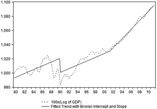
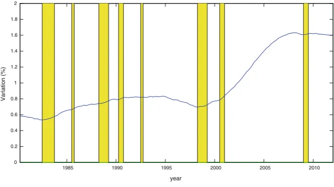
The data utilized correspond to the seasonally adjusted quarterly series11 of the logarithm of GDP from 1980 to 2011, which is shown in Fig.1. The source of information is the Peruvian Reserve and Central Bank. In terms of motivation about the presence of structural changes, Fig.1shows the possibility that the GDP may be approximated by a fitted trend with a broken intercept and a broken trend.
Peruvian GDP shows a very irregular behavior, as expected from a developing country. First, there are clear differences in the periods before and after 1990; and second, within each subperiod, the behavior of output has also been irregular, albeit less so.
In the early 1990s a process of significant economic adjustment took place, and at the same time a number of institutional reforms were enacted that drastically changed the dynamic of output. In the subperiod from 1980 to 1990, the average growth rate of GDP was approximately 0 % yearly. Large recessions occurred with an unusually high frequency and output was very volatile. In contrast, in later periods the average growth rate of GDP was more than 4 % yearly, recessions were less frequent and had a lower magnitude, and output followed a more stable path. Within each subperiod the behavior has also been irregular, as a result of recessions with varying origins and impact. For example, the 1983 recession, which was related to the ‘‘El Nin˜o’’ phenomenon and a balance of payments crisis, produced a large contraction in output that did not recover until 1985. For their part, the big recessions of 1988–1989 and 1990, associated with periods of hyperinflation and internal conflict, produced contractions in output that were not overcome until Fig. 1 Peruvian GDP and fitted broken trend
11The UC model employed can admit the series with the seasonal component; however, we choose not
1995. From then on, the recessionary periods had a lower impact, although they did not share the same nature or consequences. For example, the recession of 1998 was linked to a banking crisis that had a negative influence on the long term growth rate; the 2000 recession corresponded to a period of political instability; and the 2009 recession, associated with the international financial and economic crisis, brought about a sharp contraction in output but it was rapidly overcome. A more detailed explanation of each of these recessions is provided in Dancourt et al. (1997) and Dancourt and Mendoza (2009).
Finally, but equally important, one has to take into consideration the monetary and fiscal reforms that were implemented in the 2001–2002 period, which led to an acceleration in the rate of growth of output.
In terms of econometrics, a rigorous analysis of the series would involve a test of stationarity; that is, to find out whether the series has a stochastic trend. The advantage of utilizing disturbances with a mixture of normals lies in the fact that they allow one to model both a stochastic and a deterministic trend. For example, if the probability of being in the high variance regime is very small and the other regime has a variance close to zero, a deterministic trend is generated, with shocks that produce a change in the level or slope. Even so, a unit root test would be useful in the identification, for in the analyzed models we consider that output has a double root. Using an ADFGLS test as in Elliott et al. (1996), we observe that the null hypothesis that the series is an Ið2Þ process is rejected at 5 % but not at 1 %.12 Although this result favors a single root in output, we retain the flexible specification of (1) to (5) as it is more general and does not generate an over-identification of the models, as is explained in the next section (see, in particular, Sect.4.4).
4 Results
Before starting13 the analysis of the different models that are considered in the methodology, it is convenient to estimate a base model, UC-0, that does not include any mixture of normals, and follows the specification of Clark (1987). The obtained cycles capture the big recessions of 1988–1989 and 1990 well, but henceforward the cycle presents a positive bias; for example during the recessions of 1998 and 2009 output is above its potential or trend level. On the other hand, the cycles are long and have a large amplitude14, reaching a maximum deviation of 10 % in the mid-1990s.
12Thet-statistic—including and intercept and a time trend—forH
0:I(1) process is-1.297 implying a
non-rejection. Thet-statistic of theH0:I(2) process is-2.076 implying a rejection at 5 % but not at 1 %.
Application of a rolling ADFGLSstatistic allows similar results. However, Oh and Zivot (2006) find
evidence rejecting the imposition of two unit roots.
13
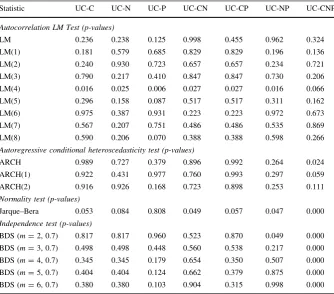
We only include tables and figures concerning the selected model (UC-CN). Other results are available upon request or they may be found in the Working Paper version; see Guille´n and Rodrı´guez (2013).
14Following definition of Castillo et al. (2007), amplitude is the distance between the maximum and
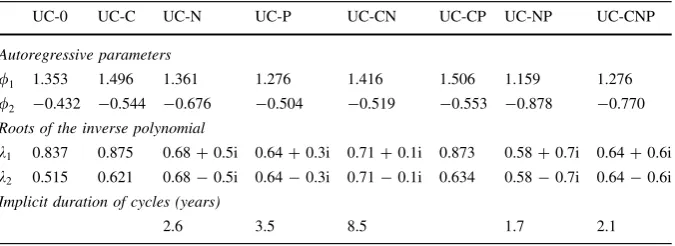
Estimations of the UC-0 model show that the cyclical component presents a large and significant standard deviation, whereas the standard deviations of the other components are close to zero. Hence, short term shocks end up explaining almost 100 % of the deviations of output. With respect to the autoregressive coefficients of the cycle, they add up to 0.932; that is, the cycle practically does not revert to mean. Besides, an analysis of its associated characteristic polynomial indicates that the roots are not complex, and hence, that the stationary component does not follow a cyclical pattern. These results, together with the upward bias in the cycles in periods after 1990, would indicate that the Clark (1987) specification does not seem adequate for modeling Peruvian GDP.
4.1 Models with one mixture of normals
Among the proposed models, the first estimation corresponds to the UC-C model that contains a mixture of normals in the disturbance of the cyclical component (t).
The cyclical component is negative during the recessive periods. Moreover, the cyclical component is most of the time below the steady state15; only during periods of high growth, as in 1986–1987 or 2008, does it take positive values. That is, there is a large asymmetry in the cycles. The obtained decomposition is similar to that which can be obtained through the ‘‘plucking’’ model of Kim and Nelson (1999a), where output grows most of the time at its potential level or ‘‘ceiling’’, and only in recessive periods does it deviate negatively from trend.
It is observed that recessions are associated mainly with periods of high variance. In contrast to the ‘‘plucking’’ model of Kim and Nelson (1999a), the observed probabilities do not correspond exactly to recession and normal periods, but rather to periods of high and low volatility. In general, the higher volatility is associated with a strong drop in output and its subsequent recovery, but can also take place in normal periods. For instance, in the first quarter of 1994, seasonally adjusted GDP grew 5.48 % and in 2002, after a brief decrease, there was a swift recovery in output and its average variation in absolute terms was of 3.53 %. This explains why those periods have a higher than 0.5 probability of being within the high variance regime. Estimations of this model reveal: the standard deviations of the disturbances, the autoregressive coefficients and the probability associated with being in the low variance regime. The existence of asymmetry in cycles is confirmed; the standard deviation of the cyclical component associated with the high variance regime (r2
2) is much higher than that associated with the low variance regime (r2
1), although the restriction admits that they can be almost equal. Both standard deviations are significant and relatively higher than the others, whereas the standard deviation of the trend level (rg) is statistically non-significant. This translates into a smooth
behavior of the trend. With respect to the autoregressive parameters (/1,/2), they
add up to 0.952; that is, short-term shocks generate cycles of high persistence or duration. On the other hand, real roots of the characteristic polynomial are obtained, and hence, the stationary component does not follow a properly cyclical pattern.
15Steady state is defined as the point at which the cyclical component is zero or GDP is exactly at its
Finally, the probability of being in the low variance regime (a1) is of 75 % and
significant; that is, the economy is most of the time in ‘‘normal’’ periods. Besides, this probability implies that the results obtained are not sensitive to the imposed restriction (probability higher than 50 %).
An additional estimation was carried out, which imposed a restriction of zero on the estimator of the standard deviation of the trend, and no major changes in the other estimators were found. On the other hand, the standard deviation of the slope is relatively small and significant, which would indicate a stable long-term growth rate. The evolution of the slope shows a decline until the early 1990s, a slight recovery during that decade, and an acceleration starting in 2000.
In order to assess the importance of short or long term shocks we weighted the variance of the cyclical component (r2
) given the probabilities, from which we
obtain that it represents 93 % of the variance in output. In contrast, the variance of the slope explains only 0.24 % of the variability of output, and the remaining percentage is explained by the shocks of the measurement equation xt. Even in
periods of low volatility, the variance of the cyclical component is higher. In other words, there is a total domination of short-term shocks on output fluctuations.
The second estimated model was an UC-N model, which contains a mixture of normals in the disturbance of the trend (gt). The observed recessionary cycles
mostly coincide with recession periods; although, in contrast to the previous model, these cycles have lower duration and amplitude. The cycles associated with the large recessions of 1988–1989 and 1990 do not show large deviations with respect to trend. However, strong drops in the trend component are observed. That is, under this specification, the drops in output during the recessions of 1988–1989 and 1990 would be associated with long term shocks that prompted abrupt changes in the trend level. The probability of being in the higher variance regime is higher during recession periods. For example, in the recession of 1998 the drop in the cycle is lower than during most of other recessions. However, this period is associated with a state of high volatility; that is, in 1998 not only a did a short-term shock take place, but also a real shock with effects in the long term.
Just as in the previous model, the periods of high volatility but no recession, such as 1994 and 2002, are related to regimes of high variance. Although in this case, they are related to long-term shocks. An important detail is the measurement of the cycle during the recession of 2009. The recessionary cycle shows a large magnitude, and the drop is even larger than that of 1998. However, the probability of a trend change is low; that is, the shock was mainly transitory.
Regarding the estimates, the standard deviation of the trend in the highest variance regime (r2
g2) is significant, just as the probability of being in a low variance regime (a1). On the contrary, the standard deviation of the lower variance regime is
non-significant (r2