Investigation of Nigerian 330 Kv Electrical Network with Distributed Generation Penetration – Part I: Basic Analyses.

(1)

Published online December, 30, 2012 (http://www.sciencepublishinggroup.com/j/ijepe) doi: 10.11648/j.ijepe.20120101.11

Investigation of nigerian 330 kv electrical network with

distributed generation penetration – part I: basic analyses

F. K. Ariyo

1,2,*

, M. O. Omoigui

1,2

1_{Department of Electronic and Electrical Engineering, Ile-Ife, Nigeria} 2_{Obafemi Awolowo University, Ile-Ife, Nigeria}

Email address:

funsoariyo@yahoo.com (F. K. Ariyo)

To cite this article:

F. K. Ariyo, M. O. Omoigui. Investigation of Nigerian 330 Kv Electrical Network with Distributed Generation Penetration – Part I: Basic Analyses. International Journal of Energy and Power Engineering. Vol. 1, No. 1, 2012, pp. 1-19. doi: 10.11648/j.ijepe.20120101.11

Abstract:

The first part of this paper presents the basic analyses carried out on Nigerian 330 kV electrical network with distributed generation (DG) penetration. The analyses include load flow, short circuit, transient stability, modal/eigenvalues calculation and harmonics. The proposed network is an expanded network of the present network incorporating wind, solar and small-hydro sources. The choice of some locations of distributed generation has been proposed by energy commission of Nigeria (ECN). The conventional sources and distributed generation were modeled using a calculation program called Po-werFactory, written by digsilent. Short-circuit analysis is used in determining the expected maximum currents, while tran-sients stability and modal analyses are considered during the planning, design and in determining the best economical oper-ation for the proposed network. One common applicoper-ation of harmonic analysis is providing solution to series resonance problems. Also, they are very valuable for setting the proper protection devices to ensure the security of the system.

Keywords:

Distributed Generation, Load Flow, Short-Circuit, Transient Stability, Modal Analysis, Eigenvalues Calcula-tion, Harmonics Analysis, Powerfactory, Digsilent

1. Introduction

Nigeria is a vast country with a total of 356, 667 sq miles (923,768 km2), of which 351,649 sq. miles (910,771 sq km or 98.6% of total area) is land. The nation is made up of six geo-political zones subdivided into 36 states and the Federal Capital Territory (F.C.T.). Furthermore, the vegetation cover, physical features and land terrain in the nation vary from flat open savannah in the North to thick rain forests in the south, with numerous rivers, lakes and mountains scattered all over the country with population of 162, 470, 737 Million people. The total installed capacity of the currently generating plants is 7, 876 MW, but the available capacity is around 4,000 MW with peak value of 4, 477.7 MW on 15th August 2012. Seven of the fourteen generation stations are over 20 years old and the average daily power generation is below 4,000 MW, which is far below the peak load forecast of 8,900MW for the currently existing infrastructure. As a result, the nation experiences massive load shedding [1-5].

This paper looks at the conventional energy generation as well as the distributed generation sources: small-hydro, solar and wind energy potentials in Nigeria. The solar, small-hydro and wind energies are ways of accelerating the

sluggish nature of the federal government of Nigeria rural electrification programmes. Nigeria receives an average solar radiation of about 7.0kWh/m2-day in the far north and about 3.5kWh/m2-day in the coastal latitudes [6]. Wave and tidal energy is about 150,000 TJ/year and the highest aver-age speeds of about 3.5 m/s and 7.5 m/s in the south and north areas respectively [7-10].

(2)

allocation are shown in Table 1 (Appendix).

However, penetration of DG can affect the stability of the system by either improving or deteriorating the stability of the system. The power system faces many problems when distributed generation is added in the already existing

sys-tem. The addition of generation could influence power quality problems, degradation in system reliability, reduc-tion in the efficiency, over voltages and safety issues [11-13].

(3)

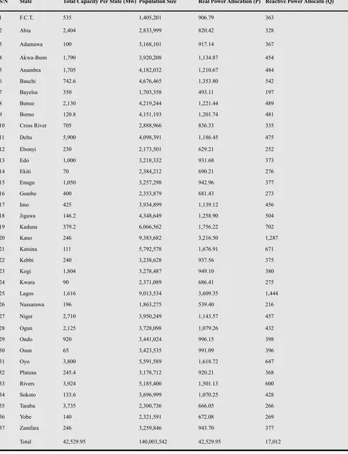
Table 1. Proposed Power generation and Allocation per State.

S/N State Total Capacity Per State (Mw) Population Size Real Power Allocation (P) Reactive Power Allocatn (Q)

1 F.C.T. 535 1,405,201 906.79 363

2 Abia 2,404 2,833,999 820.42 328

3 Adamawa 100 3,168,101 917.14 367

4 Akwa-Ibom 1,790 3,920,208 1,134.87 454 5 Anambra 1,705 4,182,032 1,210.67 484 6 Bauchi 742.6 4,676,465 1,353.80 542

7 Bayelsa 350 1,703,358 493.11 197

8 Benue 2,130 4,219,244 1,221.44 489 9 Borno 120.8 4,151,193 1,201.74 481 10 Cross River 705 2,888,966 836.33 335 11 Delta 5,900 4,098,391 1,186.45 475

12 Ebonyi 230 2,173,501 629.21 252

13 Edo 1,000 3,218,332 931.68 373

14 Ekiti 70 2,384,212 690.21 276

15 Enugu 1,050 3,257,298 942.96 377

16 Gombe 400 2,353,879 681.43 273

17 Imo 425 3,934,899 1,139.12 456

18 Jigawa 146.2 4,348,649 1,258.90 504 19 Kaduna 379.2 6,066,562 1,756.22 702

20 Kano 246 9,383,682 3,216.50 1,287

21 Katsina 111 5,792,578 1,676.91 671

22 Kebbi 240 3,238,628 937.56 375

23 Kogi 1,804 3,278,487 949.10 380

24 Kwara 90 2,371,089 686.41 275

25 Lagos 1,616 9,013,534 3,609.35 1,444 26 Nassarawa 196 1,863,275 539.40 216 27 Niger 2,710 3,950,249 1,143.57 457 28 Ogun 2,125 3,728,098 1,079.26 432

29 Ondo 920 3,441,024 996.15 398

30 Osun 65 3,423,535 991.09 396

31 Oyo 3,800 5,591,589 1,618.72 647

32 Plateau 245.4 3,178,712 920.21 368 33 Rivers 3,924 5,185,400 1,501.13 600 34 Sokoto 133.6 3,696,999 1,070.25 428 35 Taraba 3,735 2,300,736 666.05 266

36 Yobe 140 2,321,591 672.08 269

37 Zamfara 246 3,259,846 943.70 377

(4)

2. Methodology

The conventional and distributed generation sources were modeled using a calculation program called PowerFactory, written by DIgSILENT version 14.1. The name DIgSILENT stands for "DIgital SImuLation and Electrical NeTwork calculation program'' [14]. It is a computer aided engineer-ing tool for the analysis of industrial, utility, and commercial electrical power systems. It has been designed as an ad-vanced integrated and interactive software package dedi-cated to electrical power system and control analysis in order to achieve the main objectives of planning and opera-tion optimizaopera-tion.

PowerFactory works with three different classes of graphics: single line diagrams, block diagrams, and virtual instruments. They constitute the main tools used to design new power systems, controller block diagrams and displays of results. In order to meet today's power system analysis requirements, the DIgSILENT power system calculation package was designed as an integrated engineering tool which provides a complete 'walk-around' technique through all available functions, rather than a collection of different software modules [14]. Analyses carried out using Po-werFactory software in this part include load flow, transient stability, modal analysis/eigenvalues calculation and har-monics analysis. These are discussed in sections 4 – 8.

3. Network Modeling in Power Factory

The network model contains the electrical and graphical information for the grid. To further enhance manageability, this information is split into two subfolders: diagrams and network data. An additional subfolder, Variations, contains all expansion stages for planning purposes. The network model folder contains the all graphical and electrical data which defines the networks and the single line diagrams of the power system under study. This set of data is referred as the network data model. The proposed Nigerian 330 kV electrical network (37 buses), shown in Fig. 1.0, was mod-elled using this software. The DGs are limited to solar, small-hydro and wind sources. The elements data used to carry out PowerFactory analyses are shown in Appendix. The base apparent power used is 100 MVA, while the transmission line lengths (in Kilometers, Km) were per-unitized on the base value of 100 Km.

4. Load Flow Analysis

In PowerFactory, the nodal equations used to represent the analyzed networks are implemented using two different formulations:

• Newton-Raphson (current equations)

• Newton-Raphson (power equations, classical)

In both formulations, the resulting non-linear equation systems are solved by an iterative method. Load flow

cal-culations are used to analyze power systems under steady-state and non-faulted (short-circuit-free) conditions. The load flow calculates the active and reactive power flows for all branches, and the voltage magnitude and phase for all nodes under A.C. balanced, A.C. unbalanced and D.C. load flow calculation methods.

The machine currents at steady-state are calculated from [15]:

(1)

where

i = 1, 2,…, m

m is the number of generators;

i

V

is the terminal voltage of the ith generator; and

P

_i and

Q

_i are the generator real and reactive powers.

For n-bus system, the node-voltage equation in matrix form is:

(2)

Or

(3)

where

I

_bus is the vector of the injected bus currents and

bus

V

is the vector of bus voltages measured from the ref-erence node.

Y

_bus is known as the bus admittance matrix. The diagonal element of each node is the sum of admittances connected to it. It is known as self-admittance given as:

∑

= = n j ij ii y Y 0

i

j

≠

(4)

The off-diagonal element is equal to the negative of the admittance between the nodes. It is known as mutual ad-mittance, that is:

ij ji ij

Y

y

Y

=

−

(5)

A load flow calculation determines the voltage magnitude (V) and the voltage angle

( )

θ of the nodes, and the active (P)

∗ ∗ ∗ ₋ = = i i i i i i V jQ P V S I













=













nn ni n n in ii i i n i n i n i

Y

I

...

..

...

..

2 1 2 1 2 2 22 21 1 1 12 11 2 1                       n i V V V V .. .. .. 2 1 bus bus bus

Y

V

(5)

and reactive (Q) power flow on branches. The network nodes are represented by specifying two of these four quan-tities. PowerFactory uses the Newton-Raphson (power eq-uation, classical) method as its non-linear equation solver. This method is used for large transmission systems, espe-cially when heavily loaded. It was used for A.C. load flow.

From Kirchhoff’s Current law (KCL), the current at bus I is given by:

∑

= = − = n j j ij n j ij i

i V y y V

I

1 0

i

j

≠

(6)

The real and reactive powers at bus i are:

•

=

+

i i i

i

jQ

V

I

P

(7)

∑

=

+

∠

−

∠

=

−

n j j ij j ij i i i

i

jQ

V

Y

V

P

1

δ

θ

δ

(8)

∑

= + − = n j j i ij ij j i

i V V Y

P 1

)

cos(

θ

δ

(9)

∑

=

+

−

=

n j j i ij ij j i i

V

Y

Q

1

)

sin(

θ

δ

(10)

After calculating

P

_i and

Q

_i

,

the voltage and phase angle for each bus are computed iteratively using:

( ) ( ) ( )

( ) ( ) ( )k i k i k i k i k i k i

V

=

+

∆

+

=

+ + 1

1

δ

(11)

where k is the iteration step, while

∆

V

_i( )k and

∆

δ

_i( )k are calculated from Jacobian matrix. The results of the analysis are shown and discussed in section 9.

5. Short-Circuit Analysis

The short-circuit calculation in PowerFactory is able to simulate single faults as well as multiple faults of almost unlimited complexity. As short-circuit calculations can be used for a variety of purposes, PowerFactory supports dif-ferent representations and calculation (IEC60906, VCE0102, ANSI and complete) methods for the analysis of short-circuit currents. One application of short-circuit cal-culations is to check the ratings of network equipment dur-ing the planndur-ing stage. This is used in determindur-ing the ex-pected maximum currents (for the correct sizing of com-ponents) and the minimum currents (to design the protection scheme). A single phase ‘a’ to ground was introduced on a transmission line linking Niger and F.C.T. generating sta-tions using IEC60906 and ANSI methods, results are dis-cussed in section 9 [16,17].

6. Transient Analysis

The transient simulation functions available in DIgSI-LENT PowerFactory are able to analyze the dynamic beha-vior of small systems and large power systems in the time domain. These functions therefore make it possible to model complex systems such as industrial networks and large transmission grids in detail, taking into account electrical and mechanical parameters. Transients, stability problems and control problems are important considerations during the planning, design and operation of modern power sys-tems.

Short circuit switching events were created on transmis-sion line linking Niger and F.C.T. generating stations, Benue, Sokoto, Kebbi, Borno generating stations, and loss of Rivers state load. These are transient faults carried out using elec-tromechanical transients simulation method in PowerFac-tory software [11-13, 17-20].

7. Eigenvalues/Modal Analysis

The modal analysis calculates the eigenvalues and ei-genvectors of a dynamic multi-machine system including all controllers (defined before transient analysis) and power plant models. This calculation can be performed not only at the beginning of a transient simulation but also at every time step when the simulation is stopped. The eigenvalue analysis allows for the computation of modal sensitivities with re-spect to generator or power plant controllers, reactive compensation or any other equipment. The calculation of eigenvalues and eigenvectors is the most powerful tool for oscillatory stability studies. Starting from these ’bare natural’ modes, the effects of controllers (structure, gain, time con-stants etc.) and other additional models can be calculated as the second step [14].

One of the conjugate complex pair of eigenvalues is given by:

i i

j

ω

σ

λ

=

+

(12)

Then the oscillatory mode will be stable, if the real part of the eigenvalue is negative, that is,

σ

_i

〈

0

The period and damping of this mode are given by:

i i

ω

π

τ

= 2 (13)

      = − = +1 ln . 1 n n p i i A A T

d σ ₍₁₄₎

where

A

_n and

A

_n₊₁ are amplitudes of two consecutive swing maxima or minima respectively.

(6)

[14].

The absolute contribution of an individual generator to the oscillation mode which has been excited as a result of a disturbance can be calculated by:

∑

= = n i t i i i i e c t 1 ) ( φ λ

ω (15)

The nomenclature is given in Appendix.

‘c’ is set to the unit vector, that is, c = [1, ...,1], which corresponds to a theoretical disturbance which would equally excite all generators with all natural resonance fre-quencies simultaneously. The elements of the eigenvectors

i

Φ

then represents the mode shape of the eigenvalue i and shows the relative activity of a state variable, when a par-ticular mode is excited. They show for example, the speed amplitudes of the generators when an eigenfrequency is excited, whereby those generators with opposite signs in

i

Φ

oscillate in opposite phase.

The right eigenvectors

Φ

_i can thus be termed the

"ob-servability vectors''. The left eigenvectors

Ψ

_i measures the activity of a state variable x in the i-th mode, thus the left eigenvectors can be termed the "relative contribution vectors''. Normalization is performed by assigning the ge-nerator with the greatest amplitude contribution the relative contribution factor 1 or -1 respectively. For n-machine power system, n-1 generator oscillation modes will exist and n-1 conjugate complex pairs of eigenvalues

λ

_i will be

found. The mechanical speed

ω

_i of the n generators will then be described by [14]:

t nn n n n t n t n n n

i

_c

_e

_c

_e

e

c

λ λ λ

φ

ω













+













+













=













...

2 1 2 22 21 2 1 22 12 1 2 1 2 (15)

The problem of using the right or left eigenvectors for analyzing the participation of a generator in a particular mode i is the dependency on the scales and units of the vector elements. Hence the eigenvectors

Φ

_i and

Ψ

_i are combined to a matrix P of participation factor by:













Ψ

=













=

in ni i i i i ni i i i

P

p

P

.

...

.

...

2 2 1 1 2 1

φ

(16)

The elements of the matrix

P

ij are called the participa-tion factors. They give a good indicaparticipa-tion of the general system dynamic oscillation pattern. They may be used easily to determine the location of eventually needed stabilizing devices in order to influence the system damping efficiently.

Furthermore the participation factor is normalized so that the sum for any mode is equal to 1[21, 22].

8. Harmonics Analysis

One of several aspects of power quality is the harmonic content of voltages and currents. Harmonics can be analyzed in either the frequency domain, or in the time-domain with post-processing using Fourier analysis. The PowerFactory harmonics functions allow the analysis of harmonics in the frequency domain, it could be used to analyse both balanced and unbalanced network. Two different functions are pro-vided by PowerFactory [14]:

• Harmonic load flow; • Frequency sweep.

In the case of a symmetrical network and balanced har-monic sources, characteristic harhar-monics either appear in the negative sequence component (5th, 11th, 19th, etc.), or in the positive sequence component. Hence, at all frequencies a single-phase equivalent (positive or negative sequence) are used for the analysis, while for analyzing non-characteristic harmonics (3rd-order, even-order, inter-harmonics), or harmonics in non-symmetrical networks, the unbalanced option for modeling the network in the phase-domain is selected.

ency sweep is used to calculate frequency dependent impedances, the impedance characteristic can be computed for a given frequency range using ComFsweep in Power-Factory [14]. Harmonic analysis by frequency sweep is used for analyzing self- and mutual- network impedances. The voltage source models available in PowerFactory allow the definition of any spectral density function. Hence, impulse or step responses of any variable can be calculated in the frequency domain.

Balanced, positive sequence uses a single-phase, positive sequence network representation, valid for balanced sym-metrical networks. A balanced representation of unbalanced objects is used, while unbalanced, 3 Phase (ABC) uses a full multiple-phase, unbalanced network representation.

The second function is the frequency sweep performed for the frequency range defined by the ‘Start Frequency’ and the ‘Stop Frequency’, using the given Step Size. An option is available which allows an adaptive step size. Enabling this option will normally speed up the impedance calculation, and enhance the level of detail in the results by automatically using a smaller step size when required [23, 24].

9. Results and Discussion

Simulations were performed on the proposed 37-bus network using PowerFactory by DIgSILENT [14]. Tables 2-4 show results of calculation methods used which are A.C. load flow (balanced system and unbalanced) and DC load flow respectively. The base apparent power used was 100 MVA, while the transmission line lengths (in Kilometers, Km) were per-unitized on the base value of 100 Km.

(7)

re-sults-complete system report’ icon provided by the software. Secondly, short-circuit calculation was carried out on transmission line connecting F.C.T. and Niger generating stations.

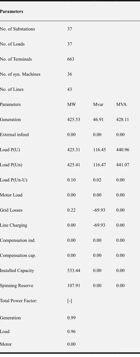
Table 2. Balanced A. C. load flow – summary report.

Parameters

No. of Substations 37 No. of Loads 37 No. of Terminals 663 No. of syn. Machines 36 No. of Lines 43

Parameters MW Mvar MVA Generation 425.53 46.91 428.11 External infeed 0.00 0.00 0.00 Load P(U) 425.31 116.45 440.96 Load P(Un) 425.41 116.47 441.07 Load P(Un-U) 0.10 0.02 0.00 Motor Load 0.00 0.00 0.00 Grid Losses 0.22 -69.93 0.00 Line Charging 0.00 -69.93 0.00 Compensation ind. 0.00 0.00 0.00 Compensation cap. 0.00 0.00 0.00 Installed Capacity 533.44 0.00 0.00 Spinning Reserve 107.91 0.00 0.00 Total Power Factor: [-]

Generation 0.99

Load 0.96

Motor 0.00

Table 3. Unbalanced A. C. load flow – summary report.

Parameters

Parameters MW Mvar MVA Generation 425.53 46.91 428.11 External Infeed 0.00 0.00 0.00 Load P(U) 425.31 116.45 440.96 Load P(Un) 425.41 116.47 441.07 Load P(Un-U) 0.10 0.02 0.00 Motor Load 0.00 0.00 0.00 Grid Losses 0.22 -69.55 0.00 Line Charging 0.00 -69.93 0.00 Compensation ind. 0.00 0.00 0.00 Compensation cap. 0.00 0.00 0.00 Installed Capacity 533.44 0.00 0.00 Spinning Reserve 107.91 0.00 0.00 Total Power Factor: [-]

Generation 0.99

Load 0.96

Motor 0.00

Table 4. D. C. load flow – summary report.

Parameters

Parameters MW Mvar MVA Generation 425.41 0.00 0.00 External infeed 0.00 0.00 0.00 Inter Grid Flow 0.00 0.00 0.00 Load P(U) 425.41 0.00 0.00 Load P(Un) 425.41 0.00 0.00 Load P(Un-U) 0.00 0.00 0.00 Motor Load 0.00 0.00 0.00 Grid Losses 0.00 0.00 0.00 Line Charging 0.00 0.00 0.00 Compensation ind. 0.00 0.00 0.00 Compensation cap. 0.00 0.00 0.00 Installed Capacity 533.44 0.00 0.00 Spinning Reserve 108.03 0.00 0.00 Total Power Factor: [-]

Generation 0.00

Load 0.00

(8)

Table 5. IEC60909 method - complete report.

Short-Circuit Duration:

Break Time 0.10 s

Fault Clearing Time 0.40 s c-Factor 1.1 Fault distance from terminal i: ... k 1.48km Fault Location (line 28) 50.00%

Phase Bus-voltage

(kV) degree c-factor Sk" (MVA)

A 0 0 1.1 1366.43 B 191.22 -107.72 0 C 193.01 110.91 0

Ik" (kA) (deg) ip (kA) Ib (kA) Sb (MVA) EFF (-)

7.17 -86.99 17.97 7.17 1366.43 0

0 0 0 0 0 0.93

0 0 0 0 0 0.9

Table 6. ANSI method - complete report.

Pre-fault Voltage 1.00 p.u.

Fault distance from terminal i: ... k 1.48 km Fault Location (line 28) 50.00% Asym.RMS X/R based [kA] 10.286 Asym. Peak X/R based [kA] 12.453

Parameters Equivalent Impedance R[Ohm] X[Ohm] Symmetrical Current [kA] [deg] App. power (MVA)

Mom.Duty 2.925 35.542 6.409 -87.74 1221.171 Zero-Seq 0.296 18.023 0 0 0 Neg.-Seq 0.297 35.542 0 0 0 Int.Duty 2.925 35.542 6.409 -87.74 1221.171 Zero-Seq 0.296 18.023 0 0 0 Neg.-Seq 0.297 35.542 0 0 0 30-cycle 4.239 53.062 5.355 -87.41 1020.274 Zero-Seq 0.296 18.023 0 0 0 Neg.-Seq 0.297 35.542 0 0 0

Parameters X/R ratio

Sym.Base [kA]

Tot.Base

[kA]

Mom.Duty 26.341 0 0 2 cycles 0 6.764 9.529 3 cycles 0 6.899 8.347 5 cycles 0 6.874 7.611 8 cycles 0 7.044 7.045

Table 7. Complete method (multiple faults).

Short-Circuit Duration:

Break Time 0.10 s Fault Clearing Time 0.40 s c-Factor 1 Fault distance

from terminal i: ... k

1.48 km Fault Location

(line 28) 50.00%

Phase

Bus Voltage (kV)

deg.

c-factor Sk" (MVA)

Ik" (kA) deg.

A 0 0 1 1198.47 6.29 -87.95 B 173.85 -107.54 0 0 0 C 174.56 110.44 0 0 0 Ik' (kA) (deg) Ip (kA) Ib (kA) Ib (kA) EFF (-) 5.22 -88.5 15.88 5.31 8.18 0 0 0 0 0 0 0.93

0 0 0 0 0 0.9

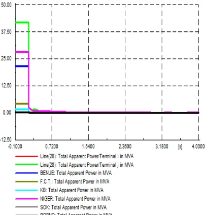
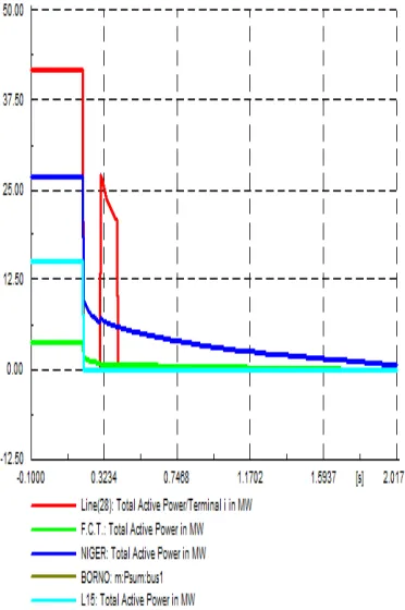
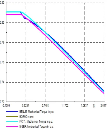
Next is transient stability analysis, short circuit switching events were created on transmission line linking Niger and F.C.T. generating stations, Benue, Sokoto, Kebbi, Borno generating station, and loss of Rivers state load using 3-phase unbalanced electromechanical transients simulation method. The switching events start by initializing the system (performing balanced load flow), followed by opening and closing phase ‘a’ of line (28) at 0.2s and 0.3s respectively and opening the three phases (‘a’, ‘b’ and ‘c’). Other com-ponents were then selected and short circuit events defined. The results are shown in Figure 2-8.

(9)

Figure 3. Turbine power (p.u.).

Figure 4. Total power factor.

Figure 5. Total active power (MW).

(10)

Figure 7. Mechanical torque (p.u.).

Figure 8. Benue hydro generating station parameters.

Next is modal analysis tool, it was used to calculate the eigenvalues and eigenvectors of a dynamic multi-machine system including all controllers and power plant models. This calculation can be performed not only at the beginning of a transient simulation but also at every time step when the simulation is stopped. A modal analysis started when a ba-lanced steady-state condition was reached in a dynamic calculation. Normally, such a state is reached by a balanced load-flow calculation, followed by a calculation of initial conditions.

Two methods were used for modal analysis: QR-method (this method is the ‘classical’ method for calculating all the system eigenvalues), while selective modal analysis method, also called Arnoldi/Lanczos calculated a subset of the sys-tem eigenvalues around a particular reference point-often used for very large system. In the later method, the reference point on the real-imaginary plain must be entered in the field

provided and the number of eigenvalues calculated is limited by the number selected at ‘Number of Eigenvalues’ field [14]. Speed was set as state variable in this paper.

The eigenvalue plots in Figure 9 and 10 show the calcu-lated eigenvalues in a two-axis coordinate system. For the vertical axis, it is possible to select among the imaginary part, the period or the frequency of the eigenvalue, while the horizontal shows the real part. Stable eigenvalues are shown in green, and unstable (none in this case) are in red. Each eigenvalue can be inspected in details by double-clicking it on the plot (in the package). This shows the index, complex representation, polar representation and oscillation para-meters of the mode. Although, in selective method, an ei-genvalue is on the imaginary axis making the system to be marginally stable.

Figure 9. Eigenvalue plot – QR method.

(11)

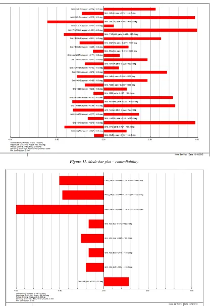
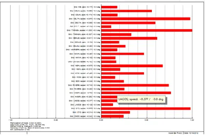
The mode bars in Figures 11, 12 and 13 show controlla-bility, observability and participation factors of variables for a user selected eigenvalue in bar chart form. This allows for easy visual interpretation of these parameters. Double

clicking on any of the bar (in the software package), displays the magnitude, phase and sign of the variables for control-lability, observability and participation in the selected mode.

Figure 11. Mode bar plot – controllability.

(12)

Figure 13. Mode bar plot - participation facto .

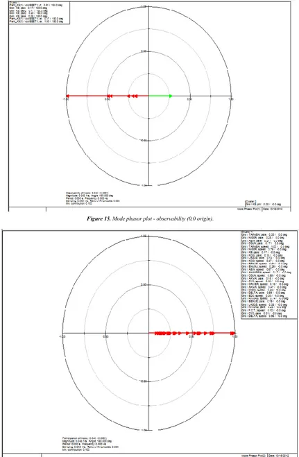
The mode phasor plot displays the controllability, obser-vability and participation factors of the system generators (according to the state variable selected in the modal analy-sis command) in a selected mode by means of a phasor diagram. Variables are grouped and coloured identically if

their angular separation is less than a user defined parameter (set at 3 degrees). Double clicking any of the bars in the plot shows the detailed dialogue as shown in Figures 14, 15 and 16.

(13)

Figure 15. Mode phasor plot - observability (0,0 origin).

(14)

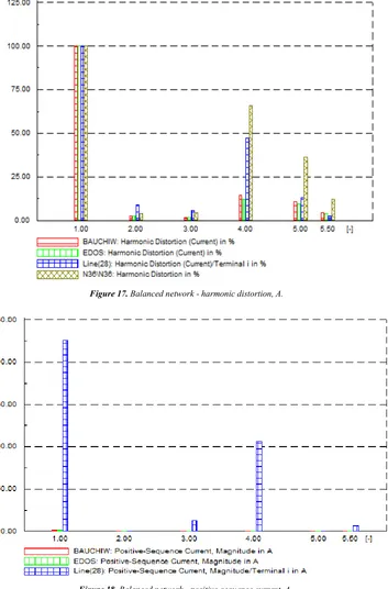
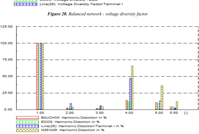
Lastly, PowerFactory’s harmonic load flow calculated actual harmonic indices related to voltage or current distor-tion, and harmonic losses caused by harmonic sources (usually non-linear loads such as current converters). Har-monic sources can be defined by a harHar-monic current or a harmonic voltage spectrum. In the harmonic load flow cal-culation, PowerFactory carries out a steady-state network analysis at each frequency at which harmonic sources are

defined. Bauchi-wind and Edo-solar generating stations, transmission line (line 28) connecting F.C.T. and Niger; Jigawa state busbar were defined for the analysis.

Frequency sweep function was used for the calculation of network impedances. The result of this calculation facilitates the identification of series and parallel resonances in the network.

Figure 17. Balanced network - harmonic distortion, A.

(15)

Figure 19. Balanced network - current diversity factor.

Figure 20. Balanced network - voltage diversity factor.

(16)

Figure 22. Unbalanced network-positive-sequence current, A.

Figure 23. Unbalanced network - current diversity factor.

(17)

Figure 25. Frequency sweep - current diversity factor.

Figure 26. Frequency sweep - harmonic distortion (current).

(18)

Figure 28. Frequency sweep - voltage diversity factor

10. Conclusion

Basic analyses were carried out in this paper (part I) and includes load flow, short-circuit calculation, transient sta-bility, modal analysis/eigenvalues calculation and harmonics analysis. Short-circuit analysis is used in determining the expected maximum currents (for the correct sizing of components) and the minimum currents (to design the pro-tection scheme), while transients, stability analyses impor-tant considerations during the planning, design and opera-tion of modern power systems. One common applicaopera-tion of harmonic analysis is providing solution to series resonance problems. These analyses have great importance in future expansion planning, in stability studies and in determining the best economical operation for the proposed network.

Nomenclature

p

i

peak current;

b

I

breaking current (RMS value);

b

i

peak short-circuit breaking current;

''

k

I

initial symmetrical short-circuit current;

b

S

peak breaking apparent power;

DC

i

decaying d.c. component;

th

i

thermal current;

op

i

load current;

kss

I

initial short-circuit current;

k

factor for the calculation of

i

_p;

m

factor for the heat effect of the d.c. component

n

factor for the heat effect of the a.c. component;

i n i

U

;

_, are nominal conditions.

)

(

t

ω

generator speed vector

i

λ

ith eigenvalue

i

φ

ith right eigenvector

i

c

magnitude of excitation of the ith mode (at t=0); n number of conjugate complex eigenvalues.

References

[1] Sambo A. S., Garba B., I. H. Zarma and M. M. Gaji, “Elec-tricity Generation and the Present Challenges in the Nigerian Power Sector”, Unpublished Paper, Energy Commission of Nigeria, Abuja-Nigeria, 2010.

[2] www.google.com/publicdata.

[3] ThisDay Newspaper, 3rd October, 2011. [4] www.energy.gov.ng.

[5] Magazine article; African Business, No. 323, Au-gust-September 2006.

[6] Ileoje, O. C. , “Potentials for Renewable Energy Application in Nigeria, Energy Commission of Nigeria”, pp 5-16, 1997. [7] Fagbenle R. L. , T. G. Karayiannis, “On the wind energy

resource of Nigeria”, International Journal of Energy Re-search. Number 18, pp 493-508, 1994.

(19)

1599-1610.

[9] Garba, B and Bashir, A. M (2002). Managing Energy Re-sources in Nigeria: Studies on Energy Consumption Pattern in Selected Areas in Sokoto State. Nigerian Journal of Re-newable Energy, Vol. 10 Nos. 1&2, pp. 97-107.

[10] M. S. Adaramola and O. M. Oyewola, ‘Wind Speed Distri-bution and Characteristics in Nigeria’, ARPN Journal of En-gineering and Applied Sciences, VOL. 6, NO. 2, FEBRU-ARY 2011.

[11] Gonzalez-Longatt F. M. , ‘Impact of Distributed generation over Power Losses on Distributed System’, 9th International Conference, Electrical Power Quality and Utilization, Bar-celona, 9-11 October, 2007.

[12] M. Begović, A. Pregelj, and A. Rohatgi, ‘Impact of Renew-able Distributed Generation on Power Systems’, Proceedings of the 34th Hawaii International Conference on System Sciences, 2001.

[13] Mohamed El Chehaly ‘Power System Stability Analysis with a High Penetration of Distributed Generation’, Unpublished M.Sc. Thesis, McGill University, Montréal, Québec, Canada, February 2010.

[14] DIgSILENT PowerFactory Version 14.1 Tutorial, DIgSI-LENT GmbH Heinrich-Hertz-StraBe 9, 72810 Gomaringen, Germany, May, 2011.

[15] Saadat H. , “Power System Analysis”, McGraw- Hill Inter-national Editions, 1999.

[16] http://webstore.iec.ch/preview/info_iec60909-0%7 Bed1.0%7Den_d.pdf.

[17] Serrican A. C. , Ozdemir A., Kaypmaz A. , ‘Short Circuit Analyzes Of Power System of PETKIM Petrochemical Aliaga Complex’, The Online Journal on Electronics and Electrical Engineering (OJEEE), Vol. (2) – No. (4), pp 336-340, Reference Number: W10-0037.

[18] Patel J. S. and Sinha M. N. ‘Power System Transient Stabil-ity Analysis using ETAP Software’, National Conference on Recent Trends in Engineering & Technology, 13-14 May 2011.

[19] Iyambo P. K. , Tzonova R. , ‘Transient Stability Analysis of the IEEE 14-Bus Electrical Power System’, IEEE Conf. 2007.

[20] Dashti R. and Ranjbar B, ‘Transient Analysis of Induction Generator Jointed to Network at Balanced and Unbalanced Short Circuit Faults’, ARPN Journal of Engineering and Applied Sciences, Vol. 3, No. 3, June 2008.

[21] Kundur P. ‘Power System Stability and Contrl’, The EPRI Power System Engineering Series, McGraw-Hill, 1994. [22] Kumar G.N., Kalavathi M.S. and Reddy B.R. Eigen Value

Techniques for Small Signal Stability Analysis in Power System Stability’, Journal of Theoretical and Applied In-formation Technology, 2005 – 2009.

[23] IEEE Recommended Practices and Requirements for Har-monic Control in Electrical Power Systems, IEEE Std. 519-1992, 1993.