Implementation of Fuzzy Rule-based Algorithms in P
Control
Chart to Improve the Performance of Statistical Process Control
Md. F. Rabbi, N. Chakrabarty, J. Shefa
Department of Industrial Engineering and Management, Faculty of Mechanical Engineering, Khulna University of Engineering and Technology, Khulna, Bangladesh.
A B S T R A C T
In the statistical process control when the process is very sensitive and the control limit shifts are the prime concerns, there the fuzzy control chart can be a better solution. In decision making, the extra ‘rather in control’ and ‘rather out of control’ decisions facilitate to find out the slight changes in the control chart. The automation of the fuzzy control chart in the Excel VBA makes the data input and decisions making process faster. The vagueness of the data is removed as the charts deal with the triangular or trapezoidal area rather than some points in the control limits. Alongside the fuzzy control charts, the Marcucci approach has been followed to find out the goodness-of-fit of the samples and to find out the effectiveness of the fuzzy control charts.
Keywords: Fuzzy control charts, Control limits, Excel VBA, Marcucci approach, Goodness-of-fit.
Article history: Received: 01 August 2018 Revised: 09 November 2018 Accepted: 03 December 2018
1. Introduction
Control charts are the preferred tools for SPC. Since 1924, when Shewhart presented, the Shewhart control charts and the various control chart techniques have been developed and widely applied in industries. The major contribution of control charts is to detect causes of defective production so that the necessary corrective actions can be taken before any large quantity of nonconforming product is manufactured. The variability of sequential data collected from a process to measure the quality characteristics reveals the existence of the common causes. So, the control charts can be used to separate out the cause of the variation, whether due to common
Corresponding author
E-mail address: [email protected] DOI:10.22105/riej.2018.128451.1040
International Journal of Research in Industrial
Engineering
causes or an assignable causes and thus determine whether the process is ‘in control’ or ‘out of control’.
Basic two types of control charts are variable control chart and attribute control chart. When the quality characteristics is measured in the numeric scale, then it is call variable control chart such as X̅-S control charts, X̅-R control charts, cumulative sum chart, etc. When the quality characteristics are measured in the qualitative form then it is called attribute control chart. The control charts of p, np, c, and u are charts for the fraction of nonconforming, nonconforming units, number of nonconformities, and nonconformities per unit, respectively; so they are attribute control chart. The quality characteristic can often be evaluated according to a binary classification of ‘conforming’ or ‘nonconforming’ depending on whether they meet the required specifications such that the number of nonconforming units can be determined. However, some amount of uncertainty or vagueness may exist due to the operator judgment variation or measurement device because the related quality characteristics are evaluated subjectively. El-Shal and Morris [3] proposed a methodology for control charting by integrating the fuzzy logic and SPC zone rules. This methodology provides a means to avoiding generation of false alarms due to random variations in the environment and/or measuring instruments and sensors. Hsu and Chen [5] applied the concept of the fuzzy sets and membership functions for softening Nelson’s rules to detect unnatural patterns of symptoms. Moreover, this group presented a new methodology used to acquire knowledge of the relationships between cause and symptoms from the data. The maximum similarity method has been used and also used the genetic algorithms for the MSM in the application of X̅ chart. Statistical Process Control (SPC) is a method used to monitor, evaluate and, improve processes in both the production and service industries to ensure process stability. A two-phase approach is followed while SPC is practiced. Phase I focuses on obtaining knowledge about the ‘in-control’ (IC) characteristics from a fixed sized data and removes the cause of the variation. On the other hand, in Phase II the process is monitored based on the estimates of the IC process parameters established in Phase I [6].
The implementation and methodologies of the quality tools are essential to alleviate items with nonconformity which results in the reduction of aggregate quality costs that enhances company’s competitive performance. Reduction of process variability can help to obtain this [7]. Control charts are very popular tools for ensuring process stability and capability [8]. This paper reports a research that has been focused on the application of fuzzy rule-based algorithms in p control chart to production lines of a garment industry.
2. Literature Review
applying the Fuzzy Operating Characteristic (FOC) curve and reached the decision that the fuzzy charts are competent for identifying process shifts and they are more efficient than the crisp chart. Zhang et al. [10] proposed a strategy to extract the controllable-domain-based fuzzy rule as a new scheme for better process control and ran a real life experiment for justification of their proposal. Naik et al. [11] proposed a Dynamic Fuzzy Rule Interpolation (D-FRI) approach which is more reliable, robust, and efficient than the conventional approach. Keivanpour et al. [12] integrated the game theory with the fuzzy rule-based approach for analyzing the strategic choice while performing the automobile manufacturers’ green end-of-life vehicle practices. The fuzzy logic is utilized as a tool for investigating a problem and analyzing the interactions and inter-relationships between its variables [4].
Cheng [13] presented a novel methodology for the fuzzy process control for the purpose of monitoring a process with the fuzzy outcomes represented by the fuzzy numbers. The out-of-control conditions of these out-of-control charts were formulated in accordance with the possibility theory. Faraz and Moghadam [14] introduced a real illustrative example, and a power test shows that designing a fuzzy control chart for the process average of a continuous (variable) quality characteristic with a warning line is a better alternative to Shewhart X̅ chart in many respects. Erginel [15] presented the theoretical structure of the fuzzy individual and moving range control charts with α cuts by considering the fuzziness that may be caused by the operator, the gauge or the environmental conditions. Colubi [16] represented a fuzzy random variable, an important role as the central summary measure, and for this reason, in the last years valuable, the statistical inferences about the means of the fuzzy random variables have been developed. Kanagawa et al. [17] used the linguistic data from a different viewpoint to construct the control chart. The presented control charts aim at controlling the process average and the variability based on an existing underlying probability distribution of the linguistic data.
3. Problem Statement
Manufacturing or production industries like garments, steels, cables, beverages, automobiles, etc. use p control chart for monitoring their products quality. But p control chart provides only yes or no decisions about their products. But only yes or is not a satisfactory decision for sampling a huge number of products. The p control chart decisions do not show the variations of samples characteristics much. Moreover, the p control chart is not automatic too. Those problems can be solved by implementing the fuzzy rules in p control charts which is proposed in this paper.
4. Theoretical Framework
Theoretical framework according to the proposed method has been described steps by steps in the following.
4.1 Fuzzy P-Control Chart Based on a Constant Sample Size for a Triangular Fuzzy Number (TFN) Case
The nonconforming fraction is defined as the ratio of the number of nonconforming units to the total number of units in that population. The units may have several quality characteristics that are examined simultaneously by the operator. If the unit does not conform to the standards for one or more of these characteristics, the unit is classified as nonconforming [26].
In the fuzzy case, the number of nonconforming units is stated using the triangular fuzzy numbers such as (daj, dbj, and dcj) based on the triangular membership function parameters (a, b, and c). In this case, the nonconforming fraction can be expressed using the triangular fuzzy numbers such as (paj, pbj, and pcj ). In this work, (pa, pb, and pc) are the fuzzy averages of the nonconforming fractions, where n is the sample size, m is the number of sample, and j = 1, 2. . . m.
𝑝𝑎𝑗=𝑑𝑎𝑗
𝑛𝑗 , 𝑝𝑏𝑗 = 𝑑𝑏𝑗
𝑛𝑗 , 𝑝𝑎𝑗 = 𝑑𝑐𝑗
𝑛𝑗 (1)
𝑝͞𝑎=∑ 𝑑𝑎𝑗
∑ 𝑛𝑗 , 𝑝͞𝑏 =
∑ 𝑑𝑏𝑗
∑ 𝑛𝑗 , 𝑝͞𝑐 =
∑ 𝑑𝑐𝑗
∑ 𝑛𝑗 (2)
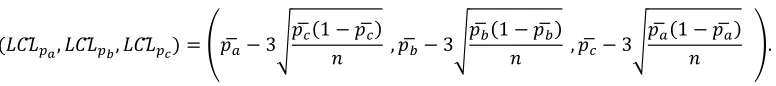
By considering the formulations of p control limits and the fuzzy numbers based on triangular membership functions, the fuzzy center line and the fuzzy upper and fuzzy lower limits of the p control chart are given as follows:
(𝑈𝐶҃𝐿𝑝𝑎, 𝑈𝐶҃𝐿𝑝𝑏, 𝑈𝐶҃𝐿𝑝𝑐) = (𝑝͞𝑎+ 3√𝑝͞𝑎
(1 − 𝑝͞𝑎)
𝑛 , 𝑝͞𝑏+ 3√
𝑝͞𝑏(1 − 𝑝͞𝑏)
𝑛 , 𝑝͞𝑐+ 3√
𝑝͞𝑐(1 − 𝑝͞𝑐)
𝑛 )
(𝐿𝐶҃𝐿𝑝𝑎, 𝐿𝐶҃𝐿𝑝𝑏, 𝐿𝐶҃𝐿𝑝𝑐) = (𝑝͞𝑎− 3√
𝑝͞𝑐(1 − 𝑝͞𝑐)
𝑛 , 𝑝͞𝑏− 3√
𝑝͞𝑏(1 − 𝑝͞𝑏)
𝑛 , 𝑝͞𝑐− 3√
𝑝͞𝑎(1 − 𝑝͞𝑎)
𝑛 ).
4.1.1 Rule for a fuzzy p-control chart based on a constant sample size for a TFN case
Rule 1. Rule 1 analyses the cases in which the fuzzy nonconforming fraction lies wholly between the fuzzy control limits or wholly outside the fuzzy control limits, as shown in Figure 1 [26].
(a) (b) (c)
Figure 1. Rules for TFN Case.
Process control state = {out of control if Pa > UCLpc Or Pc < LCLpa}in control if Pc < UCLpa And Pa > LCLpc . (4)
In Figure 1, the triangular membership function (Pc2, Pb2, Pa2) representing the process control state is ‘process in control’, and the triangular membership function (Pc1, Pb1, Pa1) representing the process control state defines the ‘process out of control’ situations.
In Figure 1(b), the triangular membership function (Pc1, Pb1, Pa1) representing the process control state is ‘rather in control’, and the triangular membership function (Pc2, Pb2, Pa2) representing the process control state is ‘rather out of control’ [2].
Process control state = {rather out of control if β < βrather in control if β ≥ β∗∗}.
β:
{
1 −Pc − UCLpa
Pc − pa if Pc > UCLpa And Pa < UCLpa
1 −LCLpc − pa
Pc − pa if Pa < LCLpc And Pc > LCLpc}
. (5)
Rule 3. Rule 3 describes the case in which the fuzzy nonconforming fraction that closes the outside to either of the control limits is a partially included corresponding control limit as shown in Figure 1(c) [1].
Process control state = {rather out of control if β < βrather in control if β ≥ β∗ ∗}.
β:
{
1 −Pc − UCLpc
Pc − pa if Pc > UCLpc And Pa < UCLpc
1 −Pc − LCLpc
Pc − pa if Pa < LCLpa And Pc > LCLpa}
. (6)
In the constant-sample-size case, the control limits and the central limits are calculated by considering the average of the sample nonconforming fractions and are calculated only once. However, if the sample size has a large variation between samples, both the upper and lower control limits should be calculated for each variable sample size.
4.1.2 Marcucci approach
Marcucci approach finds out the goodness-of-fit of the samples according to the base sample sample quality. The target value is estimated for the base period where the process is assumed to be in control. Firstly, the base sample sample standard non-conforming is expressed as
P01, P02, P03…. P0j , where j is the grade number.
The statistic to be plotted in the control chart for each sample is [2]:
𝑍𝑖2 = 𝑛𝑖𝑛0 ∑
(𝑝𝑖𝑗− 𝑝0𝑗) 𝑋𝑖𝑗− 𝑋0𝑗 , 𝑗𝑚𝑎𝑥
𝑗=1
(7)
number of samples but only on the numbers of categories. Then, the upper control limit in a generalized p-chart is the same for all multinomial processes that have the same number of categories. The control limit remains the same when the number of samples is reduced.
4.2 Fuzzy P-Control Chart Based on a Variable Sample Size for a TFN Case
If the sample size is not constant, a variable sample size should be used for calculating the control limits in a p-control chart. Two approaches exist for a variable sample size: Calculating the control limits using an approximate sample size and calculating the control limits for each sample size. n approximate sample size is used rather than a constant sample size. The following equations for the control limits given is suitable for calculating the approximate control limits [1]. However, if there is an unusually large variation in the size of a particular sample or if a point is plotted near the approximate control limits, then the exact control limits for that point should be determined and the point examined relative to that value [1]. Here, the approximate sample size is being used. Here, the fuzzy nonconforming fraction for each sample (𝑝𝑎𝑗, 𝑝𝑏𝑗, 𝑝𝑐𝑗 ) and
the fuzzy average ( 𝑝͞𝑎, 𝑝͞𝑏, 𝑝͞𝑐) are calculated as follows:
𝑝𝑎𝑗= 𝑑𝑛𝑎𝑗
𝑗 , 𝑝𝑏𝑗 = 𝑑𝑏𝑗
𝑛𝑗, 𝑝𝑎𝑗 = 𝑑𝑐𝑗
𝑛𝑗 (8)
𝑝͞𝑎 =∑ 𝑑∑ 𝑛𝑎𝑗
𝑗, 𝑝͞𝑏 = ∑ 𝑑𝑏𝑗
∑ 𝑛𝑗 , 𝑝͞𝑐 = ∑ 𝑑𝑐𝑗
∑ 𝑛𝑗
The control limits can be calculated in the fuzzy p control chart for each nj, expresses the jth sample size, uses a triangular membership function and the fuzzy average of the sample nonconforming fraction similar the way in Eq. (3).
4.2.1 Rules for fuzzy p control chart based on a variable sample size for a TFN case
Similar rules for a fuzzy p-control chart based on a constant sample size for a TFN case are defined on a variable sample size. However, the fuzzy control limit symbols include the variable sample size symbol (j). These rules are detailed as follows [1]:
Rule 1. Rule 1 analyses the cases in which the fuzzy nonconforming fraction lies completely between the fuzzy control limits or completely outside the fuzzy control limits.
Process control state = {out of control if Pa > UCLpc Or Pc < LCLpa}.in control if Pc < UCLpa And Pa > LCLpc (9)
Process control state= {rather out of control if β < βrather in control if β ≥ β∗ ∗}. (10)
β:
{
1 −Pc − UCLpa
Pc − pa if Pc > UCLpa And Pa < UCLpa
1 −LCLpc − pa
Pc − pa if Pa < LCLpc And Pc > LCLpc} .
Rule 3. Rule 3 describes the case in which the fuzzy nonconforming fraction that closes the outside to either of the control limits is a partially included corresponding to control limit.
Process control state = {rather out of control if β < βrather in control if β ≥ β∗∗}.
β:
{
1 −Pc − UCLpc
Pc − pa if Pc > UCLpc And Pa < UCLpc
1 −Pc − LCLpc
Pc − pa if Pa < LCLpa And Pc > LCLpa}
. (11)
5. Formation of Fuzzy P-Control Chart Based on a Constant and Variable Sample Size for a TFN Case
Formation of the fuzzy p-control chart based on a constant sample size and variable samples has been described sequentially in the following.
5.1 Formation of Fuzzy P-Control Chart Based on a Constant Sample Size for a TFN Case
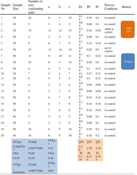
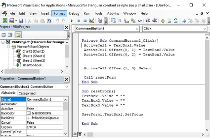
The data of the samples are taken from the different production line in Epyllion Group garments. The sample size is 50 and is constant for the all the 20 sample. The data has been processed in the excel sheet. Visual Basic coding has been moduled in the excel sheet to take the input of the data in the excel sheet.
Figure 2. Input Box.
Figure 4. Visual Basic Coding Against the ENTER Command Button.
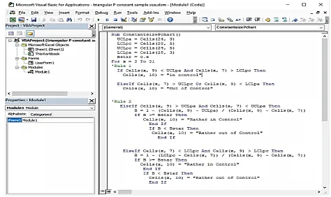
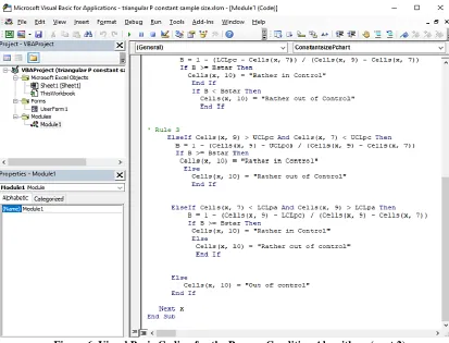
Figure 6. Visual Basic Coding for the Process Condition Algorithms (part 2).
5.2 Marcucci Approach Application for Fuzzy P-Control Chart Based on a Constant Sample Size for a TFN Case
The base sample is taken as the 4th sample as i=4 and is colored in the excel sheet where p01= 0.9, p02 = 0.06, and p03 = 0.04. All the calculations of the data are being done according to the Eq. (7). The data has been taken through the data Input Box.
Table 1. P-Control Chart Based on Constant Sample Size for TFN Case. Sample No Sample Size Number of non-conforming units
a b c Pa Pb Pc Process
Condition Button
1 50 10 8 9 10 0.1
6 0.18 0.2 in control
2 50 5 3 4 5 0.0
6 0.08 0.1 in control
3 50 13 11 12 13 0.2
2 0.24 0.26
rather in control
4 50 5 3 4 5 0.0
6 0.08 0.1 in control
5 50 8 6 7 8 0.1
2 0.14 0.16 in control
6 50 15 13 14 15 0.2
6 0.28 0.3
out of control
7 50 11 9 10 11 0.1
8 0.2 0.22 in control
8 50 10 8 9 10 0.1
6 0.18 0.2 in control
9 50 6 4 5 6 0.0
8 0.1 0.12 in control
10 50 7 5 6 7 0.1 0.12 0.14 in control
11 50 6 4 5 6 0.0
8 0.1 0.12 in control
12 50 4 2 3 4 0.0
4 0.06 0.08 in control
13 50 4 2 3 4 0.0
4 0.06 0.08 in control
14 50 8 6 7 8 0.1
2 0.14 0.16 in control
15 50 8 6 7 8 0.1
2 0.14 0.16 in control
16 50 9 7 8 9 0.1
4 0.16 0.18 in control
17 50 5 3 4 5 0.0
6 0.08 0.1 in control
18 50 5 3 4 5 0.0
6 0.08 0.1 in control
19 50 10 8 9 10 0.1
6 0.18 0.2 in control
20 50 10 8 9 10 0.1
6 0.18 0.2 in control
UCLpa UCLpb UCLp
c ∑Pa ∑Pb ∑Pc
0.2563718
3 0.285772681 0.31
2.3
8 2.78 3.18
Clpa CLpb CLpc P̅a P̅b P̅c
0.119 0.139 0.16 0.1
19 0.13 9
0.15 9
LCLpa LCLpb LCLp
c
-0.0361432 -0.00777268 0.02
Input Data
Figure 8. Visual Basic Coding for the Input Box in the Excel Sheet.
Figure 10. Visual Basic Coding for Creating P-Chart Automatically.
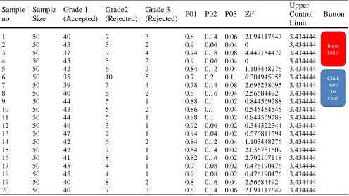
Table 3. Fuzzy P-Control Chart Based on Variable Sample Size TFN Case.
Sample no
Sample Size
Grade 1 (Accepted)
Grade2 (Rejected)
Grade 3
(Rejected) P01 P02 P03 Zi
2
Upper Control Limit
Button
1 50 40 7 3 0.8 0.14 0.06 2.094117647 3.434444
2 50 45 3 2 0.9 0.06 0.04 0 3.434444
3 50 37 9 4 0.74 0.18 0.08 4.447154472 3.434444
4 50 45 3 2 0.9 0.06 0.04 0 3.434444
5 50 42 6 2 0.84 0.12 0.04 1.103448276 3.434444
6 50 35 10 5 0.7 0.2 0.1 6.304945055 3.434444
7 50 39 7 4 0.78 0.14 0.08 2.695238095 3.434444
8 50 40 8 2 0.8 0.16 0.04 2.56684492 3.434444
9 50 44 5 1 0.88 0.1 0.02 0.844569288 3.434444
10 50 43 5 2 0.86 0.1 0.04 0.545454545 3.434444
11 50 44 5 1 0.88 0.1 0.02 0.844569288 3.434444
12 50 46 3 1 0.92 0.06 0.02 0.344322344 3.434444
13 50 47 2 1 0.94 0.04 0.02 0.576811594 3.434444
14 50 42 6 2 0.84 0.12 0.04 1.103448276 3.434444
15 50 42 7 1 0.84 0.14 0.02 2.036781609 3.434444
16 50 41 8 1 0.82 0.16 0.02 2.792107118 3.434444
17 50 45 4 1 0.9 0.08 0.02 0.476190476 3.434444
18 50 45 4 1 0.9 0.08 0.02 0.476190476 3.434444
19 50 40 8 2 0.8 0.16 0.04 2.56684492 3.434444
20 50 40 7 3 0.8 0.14 0.06 2.094117647 3.434444
Figure 11. Generalized P-Chart from Marcucci Approach for Constant Sample Size.
Sample no
Sample Size
Grade 1 (Accepted)
Grade2 (Rejected)
Grade 3
(Rejected) P01 P02 P03 Zi
2
Upper Control Limit
Button
1 50 40 8 2 0.8 0.16 0.04 3.15 3.434444
2 55 47 5 3 0.85455 0.091 0.055 0.79 3.434444
3 60 55 3 2 0.91667 0.05 0.033 0.02 3.434444
4 55 50 3 2 0.90909 0.055 0.036 0 3.434444
5 50 45 3 2 0.9 0.06 0.04 0.03 3.434444
6 45 38 5 2 0.84444 0.111 0.044 1.15 3.434444
7 34 26 5 3 0.76471 0.147 0.088 3.52 3.434444
8 45 28 13 4 0.62222 0.289 0.089 12.2 3.434444
9 65 45 15 5 0.69231 0.231 0.077 8.78 3.434444
10 54 44 7 3 0.81481 0.13 0.056 2.17 3.434444
11 52 48 3 1 0.92308 0.058 0.019 0.29 3.434444
12 44 37 5 2 0.84091 0.114 0.045 1.24 3.434444
13 47 39 5 3 0.82979 0.106 0.064 1.44 3.434444
14 54 50 3 1 0.92593 0.056 0.019 0.32 3.434444
15 55 51 3 1 0.92727 0.055 0.018 0.34 3.434444
16 48 43 3 2 0.89583 0.063 0.042 0.05 3.434444
17 49 31 15 3 0.63265 0.306 0.061 12.4 3.434444
18 50 29 15 6 0.58 0.3 0.12 15.4 3.434444
19 56 46 8 2 0.82143 0.143 0.036 2.43 3.434444
20 55 45 4 1 0.81818 0.073 0.018 0.74 3.434444
0 1 2 3 4 5 6 7
0 5 10 15 20 25
Zi
2
Sample No.
Zi2
Upper Control Limit
Click here to create
5.3 Formation of Fuzzy P-Control Chart Based on a Variable Sample Size for a TFN Case
All the algorithms have been solved the fuzzy p-control chart based on a variable sample size for a TFN case and the control chart has been drawn in the following as it was done in the constant sample size case.
Figure 12. Generalized P Chart for Variable Sample Size in Marcucci Approach.
6. Results and Discussion
6.1 Fuzzy P-Chart Based on Constant Sample Size for TFN Case and Marcucci Approach Test
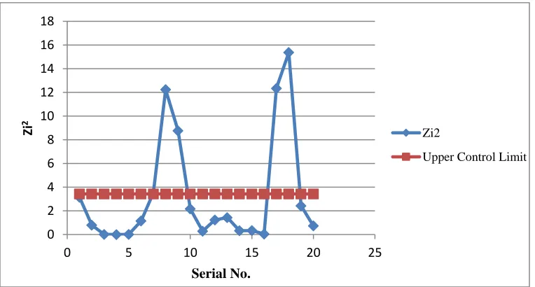
20 samples have been taken from the 20 production lines of the industry. The sample size is 50 for each of the sample. The number of non-conforming has been found 5-15 in those samples. After formulating all those data, it has been found out that the 3rd and 6th sample give the ‘rather in control’ and ‘out of control’ decision where all the other samples give the ‘in control’ decision. Again, the samples have been analyzed in the Marcucci approach and have found out the generalized p control chart. The generalized p control chart graph also shows that the 3rd and 6th sample graph just goes out of the control limit. That makes the decision that the fuzzy p chart based on constant sample size for TFN is reliable as it has given nearly same result with the goodness-of-fit test in Marcucci approach.
0 2 4 6 8 10 12 14 16 18
0 5 10 15 20 25
Zi
2
Serial No.
Zi2
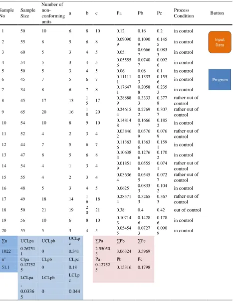
Table 4. Marcucci Approch for Variable Sample Size P-Chart. Sample No Sample Size Number of non-conforming units
a b c Pa Pb Pc Process
Condition Button
1 50 10 6 8 10 0.12 0.16 0.2 in control
2 55 8 5 6 8 0.09090
9
0.1090 9
0.145
5 in control
3 60 5 3 4 5 0.05 0.0666
7
0.083
3 in control
4 54 5 3 4 5 0.05555
6
0.0740 7
0.092
6 in control
5 50 5 3 4 5 0.06 0.08 0.1 in control
6 45 7 5 6 7 0.11111
1
0.1333 3
0.155
6 in control
7 34 8 6 7 8 0.17647
1
0.2058 8
0.235
3 in control
8 45 17 13 1
5 17
0.28888 9 0.3333 3 0.377 8
rather out of control
9 65 20 16 1
8 20
0.24615 4 0.2769 2 0.307 7
rather out of control
10 54 10 8 9 10 0.14814
8
0.1666 7
0.185
2 in control
11 52 4 2 3 4 0.03846
2
0.0576 9
0.076 9
rather out of control
12 44 7 5 6 7 0.11363
6
0.1363 6
0.159
1 in control
13 47 8 5 6 8 0.10638
3
0.1276 6
0.170
2 in control
14 54 4 1 3 4 0.01851
9
0.0555 6
0.074 1
rather out of control
15 55 4 2 3 4 0.03636
4
0.0545 5
0.072 7
rather out of control
16 48 5 3 4 5 0.0625 0.0833
3
0.104
2 in control
17 49 18 14 1
6 18
0.28571 4 0.3265 3 0.367 3
rather out of control
18 50 21 19 2
0 21 0.38 0.4 0.42 out of control
19 56 10 6 8 10 0.10714
3
0.1428 6
0.178
6 in control
20 55 5 3 4 5 0.05454
5
0.0727 3
0.090
9 in control ∑n UCLpa UCLpb UCLp
c ∑Pa ∑Pb ∑Pc
1022 0.26751
1 0 0.341
2.55050
3 3.06324 3.5969
n‾ Clpa CLpb CLpc P̅a P̅b P̅c
51.1 0.12752
5 0 0.18
0.12752
5 0.15316 0.1798 LCLpa LCLpb LCLp
c
-0.0336 5
0 0.044
Input Data
6.2 Fuzzy P-Chart Based on Variable Sample Size for TFN Case and Marcucci Approach Test
Here, the sample sizes are variable for this reason that the approximate sample size is used here. The sample sizes vary from 34 to 60 and the number of non-conforming from 5 to 21. The unexpected results come from the 8, 9, 11, 14, 15, 17, and 18th sample number. So, the process state is not so stable and the indicated sample no. gives ‘rather out of control’ or ‘in control’ decision. Marcucci approach implementation graph peaks on that points that are the main concern. As the peaks testify the validity of the fuzzy approach, so the process seems to be out of control.
7. Conclusion
Fuzzy control charts based on TFN deals with the huge number of data. The main problem that can be faced from the fuzzy control charts is the control limits shift and that can be understood from the unusual decision from the small value non-conforming numbers. On that cases, the small non-conforming units must give ‘in control’ decisions but they would give ‘rather in control’ or ‘rather out of control’ decisions; because the control limits have been shifted and the second condition of ‘in control’ decision algorithms does not satisfy the sample. The LCLd\ LCLc value becomes larger than Pa value. But to give ‘in control’ decision, the Pa value must have been larger than the LCLd\ LCLc value. That happens only in the cases when the standard deviations among the samples are very high. So, during the analysis stage of the fuzzy control chart, the unexpected decisions and their non-conforming units should be checked properly. Actually, the random variation can easily be understood and detected from the fuzzy chart. In the 20 samples, two or three ‘out of control’ decisions were acceptable but the trend of increasing of that decisions was not acceptable in the production process. The fuzzy control chart was very sensitive so shat the trend and the unusual variation can easily be detected. The Marcucci approach gived the generalized chart by comparing the other samples from the base samples. Therefore, the base sample selection was a prime factor in the graph and decision making. The base sample was an average non-conforming value contained sample in the production. Experience and intuition were integrated on the formation and decision about the fuzzy control chart.
References
Erginel, N. (2014). Fuzzy rule-based $\tilde p $ and $ n\tilde p $ control charts. Journal of intelligent & fuzzy systems, 27(1), 159-171.
Taleb, H., & Limam, M. (2002). On fuzzy and probabilistic control charts. International journal of production research, 40(12), 2849-2863.
El-Shal, S. M., & Morris, A. S. (2000). A fuzzy rule-based algorithm to improve the performance of statistical process control in quality systems. Journal of intelligent & fuzzy systems, 9(3, 4), 207-223.
Hsu, H. M., & Chen, Y. K. (2001). A fuzzy reasoning based diagnosis system for X control charts. Journal of intelligent manufacturing, 12(1), 57-64.
[6] Yang, X., Wang, Z., & Zi, X. (2017). Goodness-of-fit-based outlier detection for Phase I monitoring. Communications in Statistics - Simulation and Computation, 1–13.
Sousa, S., Rodrigues, N., & Nunes, E. (2017). Application of SPC and quality tools for process improvement. Procedia manufacturing, 11, 1215-1222.
Kaya, I., Erdoğan, M., & Yıldız, C. (2017). Analysis and control of variability by using fuzzy individual control charts. Applied soft computing, 51, 370-381.
Fadaei, S., & Pooya, A. (2018). Fuzzy U control chart based on fuzzy rules and evaluating its performance using fuzzy OC curve. The TQM journal, 30(3), 232-247.
Zhang, B., Yang, C., Zhu, H., Shi, P., & Gui, W. (2018). Controllable-domain-based fuzzy rule extraction for copper removal process control. IEEE transactions on fuzzy systems, 26(3), 1744-1756. Naik, N., Diao, R., & Shen, Q. (2018). Dynamic fuzzy rule interpolation and its application to intrusion detection. IEEE transactions on fuzzy systems, 26(4), 1878-1892.
Keivanpour, S., Ait-Kadi, D., & Mascle, C. (2017). Automobile manufacturers’ strategic choice in applying green practices: joint application of evolutionary game theory and fuzzy rule-based approach. International journal of production research, 55(5), 1312-1335.
Cheng, C. B. (2005). Fuzzy process control: Construction of control charts with fuzzy numbers. Fuzzy sets and systems, 154(2), 287-303.
Faraz, A., & Moghadam, M. B. (2007). Fuzzy control chart a better alternative for Shewhart average chart. Quality & quantity, 41(3), 375-385.
Erginel, N. (2008). Fuzzy individual and moving range control charts with α-cuts. Journal of intelligent & fuzzy systems, 19(4, 5), 373-383.
Colubi, A. (2009). Statistical inference about the means of fuzzy random variables: Applications to the analysis of fuzzy-and real-valued data. Fuzzy sets and systems, 160(3), 344-356.
Kanagawa, A., Tamaki, F., & Ohta, H. (1993). Control charts for process average and variability based on linguistic data. The international journal of production research, 31(4), 913-922.
Kaya, İ., & Kahraman, C. (2011). Process capability analyses based on fuzzy measurements and fuzzy control charts. Expert systems with applications, 38(4), 3172-3184.
Faraz, A., & Shapiro, A. F. (2010). An application of fuzzy random variables to control charts. Fuzzy sets and systems, 161(20), 2684-2694.
Laviolette, M., Seaman, J. W., Barrett, J. D., & Woodall, W. H. (1995). A probabilistic and statistical view of fuzzy methods. Technometrics, 37(3), 249-261.
Marcucci, M. (1985). Monitoring multinomial processes. Journal of quality technology, 17(2), 86-91.
Saaty, T. L. (1974). Measuring the fuzziness of sets. Taylor & Francis, 4(4), 53-61.
Wang, J. H., & RAZ, T. (1990). On the construction of control charts using linguistic variables. The international journal of production research, 28(3), 477-487.
Woodall, W. H. (1997). Control charts based on attribute data: Bibliography and review. Journal of quality technology, 29(2), 172-183.
Woodall, W. H., Tsui, K. L., & Tucker, G. R. (1997). A review of statistical and fuzzy quality control charts based on categorical data. Frontiers in statistical quality control (pp. 83-89). Physica, Heidelberg.