http://www.sciencepublishinggroup.com/j/ijgg doi: 10.11648/j.ijgg.20170503.11
ISSN: 2376-7340 (Print); ISSN: 2376-7359 (Online)
Identification of Individuals in a DNA Mixture Using SNP
Markers
Abdulwasiu Ibrahim
School of Public Health, University of the Witwatersrand, Johannesburg, South Africa
Email address:
1708336@students.wits.ac.za
To cite this article:
Abdulwasiu Ibrahim. Identification of Individuals in a DNA Mixture Using SNP Markers. International Journal of Genetics and Genomics. Vol. 5, No. 3, 2017, pp. 27-35. doi: 10.11648/j.ijgg.20170503.11
Received: April 9, 2017; Accepted: April 24, 2017; Published: July 10, 2017
Abstract:
This article focuses mainly on DNA mixture from two contributors, a victim and an unknown culprit. There are two areas I believe will be of interest to forensic scientists, police and a Jury. These areas are identification of an individual in a DNA mixture and familial DNA database searching of a culprit through a relative. In this article, I looked at identification of individuals in a mixture using Single Nucleotide Polymorphisms (SNPs) markers. SNPs are starting to be used for forensic identification; I employed them as they produce incredible results for identification in a two-person mixture. The conservative method I employed here is the random man not excluded probability – P (RMNE) approach, an inclusion probability method generally considered as a frequentist approach. It was found that an optimum allele frequency of 0.2 is required to produce almost certain identification with much distortion in identifying an individual even when inbreeding is up to 50% in a population. Another interesting thing is that relatives of a suspect whom are actual contributors to the DNA mixture can also be identified. In a case where there are relatives in the mixture it was found that twice the number of SNP panels is required to identify an individual than in a case where no relative is involved. And lastly, typing more SNP panels helps to improve identification and therefore produce forensically useful results.Keywords:
SNP Markers, DNA Mixture, Allele Frequency, Likelihood Ratio, Hardy-Weinberg Equilibrium1. Introduction
The use of Single Nucleotide Polymorphisms (SNPs) markers in human identification is fast growing in the forensic field as the attention of forensic scientists and researchers is being drawn to this marker. SNP markers are the most abundant in the human genome. These make it easy to multiplex hundreds of thousands of them. They have a fairly low mutation rate compared to Short Tandem Repeat (STR) markers which is an advantage in terms of genetic stability which brightens the future of SNP markers for forensic work [1].
It is a known fact that SNPs are one of the most common genotyping markers apart from STR loci, which are the predominant loci used for identification. The crimes databases kept by countries were typed using STR loci. However, there are some draw backs to when STR loci are used. For instance, if I have a degraded DNA sample from a mass disaster, say from a plane crash, it will be difficult to
obtain genetic information from this sample. This degraded DNA sample means that when typed with STR loci, little or no genetic information is obtained (which is not informative). Consequently, STR mitochondria DNA typing was developed to take care of the lapses caused by degraded DNA samples, though it is costly and time consuming [2]. This is where SNP markers come in. They are relatively cheap and less time consuming because of their abundance in the genome, yet they provide adequate genetic information needed as appropriate from a degraded sample.
unreliable for mixture interpretation, the possibilities of SNP taking over as the predominant marker for human identification in forensic case work is still far from possible.
However, more recently, researchers and forensic scientists have started to come out with methods for identification of humans in a mixture with SNP genotyping [6, 7]. A paper by Voskoboinik and Darvasi [8] presented a frame work that requires typing between 1000 and 3000 SNP panels, each with relatively low minor allele frequency, the idea being that an individual is expected to carry dozens of rare alleles, and this set of alleles will be carried in the complex mixture provided an individual with the alleles is a contributor to the mixture.
Voskoboinik and Darvasi [8] have tried to look at a mixture of up to ten contributors, different numbers of independent SNPs and varying minor allele frequencies. As said from previous chapters I shall only be considering a two-person mixture, and this will not change. However, there are other areas which I think will be of interest to look at; these include consanguinity in the population through incorporation of an inbreeding model. I will look at how results compare in both consanguineous and non-consanguineous populations. Another thing they looked at in the article is the presence of a close relative (brother) in the mixture; I shall extend it to look at fathers.
2. Materials and Method
The Likelihood Ratio (LR) [9] is the most widely used recommended approach for interpretation of mixtures. It is case specific in the sense that it requires the profile of an arrested suspect or profile of a database person to be compared with the mixture in order to calculate the likelihood ratios. However, there is a frequentist approach to the interpretation of the mixture; this approach is called the Random Man Not Excluded-RMNE approach.
The RMNE method is mainly a probability calculation -P(RMNE), where a random person would not be excluded as a contributor to an observed DNA mixture, also known as the Inclusion probability [10].
Unlike the likelihood ratio, P (RMNE) is rather a
conservative approach which will produce similar results as a likelihood ratio provided there are no dropouts and genotyping errors are avoided.
The Random man not excluded probability is given by [8]:
(
)
( )l ( ) n ( )
P RMNE = P ij ×P ij (1) where n is the number of contributors at locus l, so for a two-person contributor to a mixture it will be written as
(
)
2( )l ( ) ( )
P RMNE = P ij ×P ij . The multi-locus random man not excluded probability across L SNP panels will then be written as
(
)
(
2)
1
( ) ( ) ( )
L
l
P RMNE P ij P ij
=
=
∏
× (2)Note that this requires an estimate of genotype frequency. The basic thing about this approach is that we are only interested in the overall P(RMNE) calculation. One needs to make sure that there are no exclusions by making sure that we do not miss out any genotype at each mixture profile. Since SNP markers are not as polymorphic as their STR loci counterparts, the maximum mixture length is two (mixture profile AB) for any SNP panel; this makes it easy to follow through. Table 1 contains the entire genotype possibilities of a random man not excluded for each mixture scenario with their probabilities we sum them together to give an overall random man not excluded probability. The smaller the value of the P(RMNE) the bigger, we would expect the evidence to be that a suspect is an actual contributor to the DNA mixture given that a non-DNA evidence has been established against the suspect. So P(RMNE) is a way to find how many loci are needed for strong evidence. We cite an instance of how to go about the calculation in Table 1, taking for example mixture AB and a typed victim with genotype AA. Upon seeing this mixture and victim profiles, allele ‘B’ must be coming from the culprit which could either mean the culprit has AB or BB genotype. For each of AB or BB that could be the culprit’s genotype, a RMNE will have genotypes AB or BB. So P(RMNE) under a mixture AB and victim AA is;
(
)
(
)
{
P AA( )×P BB( )× P AB( )+P BB( ) +P AA( )×P AB( )× P AB( )+P BB( )}
(3) Assuming Hardy-Weinberg equilibrium;2 2 2 3 2
( 2 ) 2 ( 2 )
A B B A B A B B A B
P P P + P P + P P P + P P (4) We decided to split it into in Table 1 so as to follow through easily. The reason that most suspects prefer evidence
to be calculated using the RMNE approach is that since the defence hypothesis is usually never known; it does not depend on or make use of the suspect’s DNA profile [10]. It is far easier than a likelihood ratio to explain to the jury whom may not have an idea of how the calculations work.
Table 1. P(RMNE) for unrelated two-person mixture (Assuming Hardy-Weinberg).
Mixture profile Victim profile Culprit profile RMNE Inclusion Probability
A AA AA AA 6
A
P
B BB BB BB 6
B
P
AB AA BB BB or AB
2 2 2
(1 )
A B A
P P −P
Mixture profile Victim profile Culprit profile RMNE Inclusion Probability
BB AA AA or AB
2 2 2
(1 )
A B B
P P −P
AB AA or AB 2 3(1 2)
A B B
P P −P
AB
AA AA or BB or AB 3
2P PA B
BB AA or BB or AB 3
2P PA B
AB AA or BB or AB 2 2
4P PA B
Overall Inclusion Probability P(RMNE) 6 6 2 2 2 2 3 2 3 2
(6 ) 2 (2 ) 2 (2 )
A B A B A B A B A A B B
P +P +P P −P −P + P P −P + P P −P
3. Results and Discussion
3.1. Effect of Minor Allele Frequencies and Different Number of SNP Panels on Random Man Not Excluded Probability
Using Table 1 we intend to look at how minor allele frequencies and different numbers of SNP panels affect the P(RMNE) calculation. As I have stated in Section 2 above, as the value of P(RMNE) becomes smaller the more the evidence that an arrested suspect does contribute to the mixture. Small values between zero and one would not be very easy to keep track of so we have converted to the – log scale for convenience. We see from Figure 1 that when more SNP panels are used there is a great and significant impact on the improvement of – log P(RMNE). Foreman and Evett [11] proposed in their paper that a value of 10-9 as the standard report match probability for a ten locus STR system. A value of 10-9 for P(RMNE) can also be said with utmost certainty that a suspect not excluded from being a contributor to a mixture is actually a contributor to the DNA mixture [8]. If we are to go by this, then a 100 SNP panel will be sufficient to say a suspect not excluded from being a contributor to a mixture is actually a contributor to the DNA mixture. The relationship between –log P(RMNE) on the y-axis and different numbers of SNPs on the x-axis is linear (as SNPs increase the value of –log P(RMNE) increases as well).
As allele frequencies are important in STR loci, so are they in SNP panels. Different populations may have different
allele frequencies for the SNP and the calculation of random man not exclude probability depends on it. If one of the two allele frequencies is known, then the second is one minus the allele frequency of the first. We did look at a range of allele frequencies (0.1 – 0.5) in the calculations of P(RMNE). Budowle and van Daal [2] proposed using allele frequencies close to 0.5, the reason was for an increase in statistical power, but the graph in Figure 1 was able to show that an allele frequency of 0.5 leads to a decrease in –log P(RMNE). An allele frequency of 0.2 stood out amongst others to be optimal as in increasing the value of –log P(RMNE), even as the number of SNPs increases it improves the value of –log P(RMNE) progressively as well.
Voskoboinik and Darvasi [8] gave the equation of calculating optimal the minor allele frequency as;
1
1 n MAF
n = −
+ (5)
where n is the number of contributors
Upon inserting n=2 into that equation MAF=0.18, which is approximately 0.2, and this further confirms the optimality of the allele frequency of 0.2 and the essence of finding the right allele frequencies. As can be seen from both Figures 1 and 2 the 0.5 allele frequency shows the least improvement in –log P (RMNE) as the SNP panel increases. From now on we will focus on allele frequencies 0.2 and 0.5. We will see how these two allele frequencies fare when we consider other components like consanguinity and close relatives in the mixture in the coming sub sections.
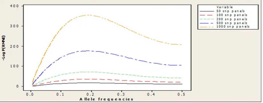
Note that the plot in Figure 2 is an extension of Figure 1 simply by looking at a number of allele frequencies from 0.005 through 0.5 with an interval of 0.005 between them. We are able to find out that allele frequencies above 0.06 will do better at identifying an individual in a DNA mixture.
However, the bone of contention here for us is to find the right allele frequencies in order to accurately estimate the P(RMNE). We have seen that 0.2 is good for the simple setting, but what about the other settings?
Figure 2. Density plot of –Log P(RMNE) as a function of minor allele frequencies for different number SNP panels.
3.2. Effect of Consanguinity in the DNA Mixture
Bittles and Saggar [12] gave estimates of consanguinity in the populations in the world with North America, Western Europe and Oceania having the least consanguineous marriage rate <1%. Southern Europe, Japan and South America have between 1 and 5%. Consanguineous marriage is at its peak in the Middle East (Arab Nations) and parts of North Africa which can be up to 50% or more. With consanguineous marriage will come excess homozygosity in the population, which leads to deviation from Hardy-Weinberg equilibrium. In order for it to be valid inbreeding has to be incorporated into the genotype proportions.
( ) A( (1 ) A)
P AA =P f + −f P (6)
( ) 2 A B(1 )
P AB = P P − f (7) where f is the inbreeding coefficient.
A look at Table 2 shows that it takes the same format as Table 1 only that inbreeding has been incorporated into the Hardy-Weinberg proportions. If f is set to zero it is exactly the same as the contents of Table 1.
In Figure 3 (a) different levels of f were looked into as consanguinity varies between populations. The levels of inbreeding considered were 1%, 10%, 20% and 50%. A population such as that of the UK with an inbreeding coefficient
≤
1% can still be tagged as no consanguinity (f = 0) because there is no reasonable difference between it and when f = 0. The same thing that applies to the case when f = 0 is seen for f = 0.01, which is again an allele frequency of 0.2 represents the optimum.As can be seen in Figure 3 (b) and (c), the picture looks fairly similar, though as we move towards an allele frequency of 0.5 there is a significant improvement in the value of –Log P(RMNE). This can be seen clearly in Figure 3 (c) suggesting that an increase in f will lead to an increase in –Log P(RMNE) value as we move towards the 0.5 allele frequency. Another thing that might be of interest is that when an allele frequency of 0.2 was looked at for all values of the inbreeding coefficient, there does not seem to be much difference in the corresponding value of –Log P(RMNE), unlike what we noticed in the case of the 0.5 allele frequency.
The plot for Figure 3 (d) looks very much like a projectile motion which attained a maximum height at allele frequency of 0.25 and remained steady up and till allele frequency of 0.5. One thing can be said of this is that in a population where consanguineous marriage persists reaching up to 50%, a higher choice of allele frequencies is preferred in order to identify effectively individuals in a mixture.
Table 2. P(RMNE) for unrelated two-person mixture with incorporation of inbreeding.
Mixture profile Victim profile Culprit profile RMNE Inclusion Probability
A AA AA AA PA
(
f + −(1 f P) A)
3B BB BB BB PB
(
f + −(1 f P) B)
3AB
AA BB BB or AB ( ) ( ) ( )
2
(1 ) . (1 ) . 1 (1 )
A B A B A
P P f+ −f P f + −f P + −f P
AB BB or AB 2 2( ) ( ) ( )
2P PA B f + −(1 f P) A . 1−f . 1 (1+ −f P) A
BB AA AA or AB ( ) ( ) ( )
2 (1 ) . (1 ) . 1 (1 )
A B A B B
P P f+ −f P f + −f P + −f P
AB AA or AB 2 2( ) ( ) ( )
2P PA B f + −(1 f P) B . 1−f . 1 (1+ −f P) B
AB
AA AA or BB or AB 2
(
)
{
(
)
(
)
}
2P PA B(1−f). f+ −(1 f P) A . PA f+ −(1 f P) A +PB 1 (1+ −f P) A
BB AA or BB or AB 2P PA B2(1−f).
(
f+ −(1 f P) B)
.{
PA(
f+ −(1 f P) A)
+PB(
1 (1+ −f P) A)
}
AB AA or BB or AB 4P PA2 B2(1−f) .2{
PA(
f+ −(1 f P) A)
+PB(
1 (1+ −f P) A)
}
Overall Inclusion Probability P(RMNE)
( )
(
)
(
( ))
( ) ( ) ( )( )
( ) ( )
3 3
2 2
2 2
2
(1 ) (1 )
(1 ) . 1 (1 ) (1 ) 1 (1 )
2 (1 ) (1 ) 1 (1 )
A A B B
A B A A A B B B
A B A A B A
P f f P P f f P
P P f f P f P P P f f P f P
P P f P f f P P f P
+ − + + − +
+ − + − + + − + − +
− + − + + −
The choice of 0.5 allele frequency will not be good in a population with low consanguinity for identifying individuals in a two-person mixture. An unmistakable fact is that increasing SNP panels will increase –log P(RMNE) for identification in the mixture even when consanguinity is at its peak. When the number of SNP panels is doubled there is a corresponding double effect on –log P(RMNE) value (higher value shows that an arrested suspect truly is a contributor of the DNA mixture).
Figure 3a. Plot of –Log P(RMNE) as a function of minor allele frequencies for different number SNP panels when inbreeding coefficient (f) is 0.01.
Figure 3c. Plot of –Log P(RMNE) as a function of minor allele frequencies for different number SNP panels when inbreeding coefficient (f) is 0.2.
Figure 3d. Plot of –Log P(RMNE) as a function of minor allele frequencies for different number SNP panels when inbreeding coefficient (f) is 0.5.
Figure 4. A clustered bar chart showing –Log P(RMNE) on the y-axis and level of consanguinity (f = 0, f = 0.01, f = 0.1, f = 0.2 and f = 0.5) in the mixture when considering allele frequencies of 0.2 and 0.5 for 500 and 1000 SNP panels (both on x-axis).
3.3. Effect of the Suspect’s Relative in the DNA Mixture
Two close relative that can be investigated are the parent and sibling. These two relations were the only ones looked at in earlier chapters and this chapter will not be an exception. In a case where a crime was committed by the father or the brother of the arrested suspect, the random man not excluded probabilities are calculated for each of the relations simply
Table 3. Parentage Likelihood ratio for different combinations of genotype.
Child Father Likelihood Ratio
AA AA 1
A P
AA AB 1
2PA
AB AA 1
2PA
AB AC 1
4PA
AB AB 1 1
4PA 4PB
+
AA BB
0
AA BC
AB CD
Table 4. Sibling Likelihood ratio for different combinations of genotype.
First sibling Second sibling Likelihood Ratio
AA AA 2
1 1 1
4 2PA 4PA
+ +
AA AB 1 1
4 4PA
+
AB AC 2
1 1 1
4 2PA 4PA
+ +
AB AB 1 1 1 1
4 8PA 8PB 8P PA B
+ + +
AA BB
1 4
AA BC
AB CD
I was able to produce a plot using 500 and 1000 SNP panels for different values of allele frequencies from 0.005 through 0.5. This is shown in Figure 5 for relations and no relations in the mixture. As can be seen from the figure, when there is no relation of the suspect half of SNP panels required to identify a relation is needed, so far inclusion of a relative like father and brother, twice the number of SNP panels for no relation is needed. The plot in figure 5 seems to be partitioned into 3 segments. Upon looking at the mid segment (containing 1000 SNPs-father, 1000 SNPs-brother and 500 SNPs- no relative) we can see that the three relations in this segment follow almost the same line from 0.05 till it reaches the optimum point at 0.2, then there is a gradual decrease as we move along other allele frequencies.
Lastly, a clustered bar chart was put in place to compare the 0.2 and 0.5 allele frequencies for the different relationships, Figure 6. We can see that the choice of the 0.2 allele frequency has the upper hand at improving the value of –log P(RMNE) in identification of an individual in a mixture compared to the 0.5 allele frequency. The highest value of – log P(RMNE) came for 0.2 an allele frequency under no relatives in the mixture, confirming what we saw in Figure 5 with the others trailing behind. Another thing is that if there are no relatives in the mixture one can still use 0.5 allele frequency because the –log P(RMNE) produced for identification is higher than when there is a relative of the suspect in the mixture (but it is not as good as 0.2). Identification of a father in a mixture is slightly better than a brother.
Figure 5. Density plot of –Log P(RMNE) as a function of minor allele frequencies for comparison among the three relationships (no relative, a father and a brother) in the mixture considering only 500 and 1000 SNP panels.
Table 5. P(RMNE) of a father being part of the two-person mixture (Assuming Hardy-Weinberg).
Mixture profile Victim profile Culprit profile RMNE Inclusion Probability
A AA AA AA 5
A P
B BB BB BB 5
B
P
AB
AA BB BB or AB
2 2 A B P P
AB BB or AB P P PA3 B( B+1)
BB AA AA or AB
2 2 A B P P
Mixture profile Victim profile Culprit profile RMNE Inclusion Probability
AB
AA AA or BB or AB 3
2P PA B
BB AA or BB or AB 2 3
A B P P
AB AA or BB or AB 2 2
4P PA B
Overall Inclusion Probability P(RMNE) 5 5 2 2 3 3
6 ( 3) ( 3)
A B A B A B B A B A
P +P + P P +P P P + +P P P +
Table 6. P(RMNE) of a sibling being part of the two-person mixture (Assuming Hardy-Weinberg).
Mixture profile Victim profile Culprit profile RMNE Inclusion Probability
A AA AA AA 6 2
1 1 1
.
4 2 4
A A A P P P + +
B BB BB BB 6
2
1 1 1
4 2 4
B B B P P P + + AB AA
BB BB or AB 2 4 2 3 3
1 1 1 1 1
2
4 2 4 4 4
A B A B
B B B
P P P P
P P P
+ + + +
AB BB or AB 2 3 3 1 1 4 4 2 1 1 1 1
4 4 4 8 8 8
A B A B
B A B A B
P P P P
P P P P P
+ + + + +
BB
AA AA or AB 4 2 2 3 3
1 1 1 1 1
2
4 2 4 4 4
A B A B
A A A
P P P P
P P P
+ + + +
AB AA or AB 2 3 3 1 1 4 2 4 1 1 1 1
4 4 4 8 8 8
A B A B
A A B A B
P P P P
P P P P P
+ + + + +
AB
AA AA or BB or AB 3
2P PA B
BB AA or BB or AB 2P PA B3
AB AA or BB or AB 4 2 2
A B P P
Overall Inclusion Probability P(RMNE)
{
2 4 2 2 2 4 2 2}
3 2 2 3 3 3
3 3 2 2
1
( 2 1).( ) ( 2 1).( )
4
( 1) ( 1) ( 1).( )
2 2 4
A A A A B B B B A B
A B B A B A A B A B A B
A B A B A B
P P P P P P P P P P
P P P P P P P P P P P P
P P P P P P
+ + + + + + + + + + + + + + + + +
Figure 6. A clustered bar chart showing –Log P(RMNE) on the y-axis and three relationships (no relative, a father and a brother in the mixture when considering allele frequencies of 0.2 and 0.5 for 500 and 1000 SNP panels (both on x-axis).
4. Conclusion
The conservative approach of Random man not excluded probability P(RMNE) used in this chapter for two person-mixtures was able to give us a clue into finding the right and optimum allele frequency to use. The magnitude of P(RMNE) depends on the allele frequency that has been
used. A 0.2 allele frequency is considered to be good enough to produce the expected random man not excluded probability based results produced in our simulations and equation (6) of the Voskoboinik and Darvasi [8] article.
relative of the suspect contributes to the mixture, a lower value of the -log P(RMNE) is produced compared with when there is no relative in the mixture, but increasing the number of typed SNP panels can address this and thereafter improve identification.
Acknowledgement
The author thanks Dr. Karen Ayres for the supervisory role and assistance in writing the R-codes.
References
[1] Butler, J. M., M. D. Coble, and P. M. Vallone, STRs vs. SNPs: thoughts on the future of forensic DNA testing. Forensic Science, Medicine, and Pathology, 2007. 3(3): p. 200-205. [2] Budowle, B. and A. van Daal, Forensically relevant SNP
classes. Biotechniques, 2008. 44(5): p. 603-8, 610.
[3] Mo, S.-K., et al., Exploring the efficacy of paternity and kinship testing based on single nucleotide polymorphisms. Forensic Science International: Genetics, 2016. 22: p. 161-168.
[4] Rapley, R. and S. Harbron, Molecular analysis and genome discovery. 2011.
[5] Kidd, K. K., et al., Developing a SNP panel for forensic identification of individuals. Forensic Sci Int, 2006. 164(1): p. 20-32.
[6] Egeland, T., I. Dalen, and P. F. Mostad, Estimating the number of contributors to a DNA profile. Int J Legal Med, 2003. 117(5): p. 271-5.
[7] Egeland, T., et al., Complex mixtures: A critical examination of a paper by Homer et al. Forensic Science International: Genetics, 2012. 6 (1): p. 64-69.
[8] Voskoboinik, L. and A. Darvasi, Forensic identification of an individual in complex DNA mixtures. Forensic Sci Int Genet, 2011. 5(5): p. 428-35.
[9] Rudin, N. and K. Inman, Likelihood Ratio and Probability of Exclusion, in An Introduction to Forensic DNA Analysis, Second Edition. 2001, CRC Press.
[10] Buckleton, J., C. M. Triggs, and S. J. Walsh, Forensic DNA Evidence Interpretation. 2004: CRC Press.
[11] Foreman, L. A. and I. W. Evett, Statistical analyses to support forensic interpretation for a new ten-locus STR profiling system. Int J Legal Med, 2001. 114 (3): p. 147-55.