The Calculation of Solar Cells with the Function of H – Geometry

The Calculation of Solar Cells with the Function of H – Geometry

Dr. Donaldas Zanevičius

President of Lithuanian Engineers Association Space Technology Research Center, Chairman of Scientific Council

Tuskulenu street 7 – 84, LT-09216 Vilnius Lithuania

Abstract

When the function exp is used for diode volt-amperes characteristic, then the volt-amperes characteristic of Solar cells cannot be calculated using standard computer programs. Therefore, special algorithms and programs are developed. If the diode volt-amperes characteristic is described by geometrical progression function of tph, the volt imperial characteristic of Solar cells is described by second grade algebraic equation, which solution is easily calculated by an analytical function. Using the geometrical progression function the calculations of transistor schemes also significantly deteriorates.

Introduction

Calculating the nonlinear electronic circuits containing p-n junction there appear problems in realization of calculation algorithms. One of these widely used circuits is element of the Sun. In recent years, solar cells (SC) as an alternative energy particle are further explored in various scientific journals. After selecting the equivalent scheme the mathematical model is written. In most cases, the p-n junction volt amperes characteristic is described by transcendental function exp. Therefore equation is obtained transcendental [1]

i Ip Ieo e u i Rs



1

 

 

   

 ui Rs

Rp



(1)

Rp here is shunt resistance, o Rs – consistent resistance. Ip – power generator flow.

Equation (1) – one diode model. To find an analytical expression from (1) or directly digital methods to calculate the characteristics of the SC volt amperes

i f u( )

is not possible as in the transcendental equation (1) the flow i and voltage u are in exp rate and fraction. Such transcendental equations are solved by devising special digital algorithms and programs [2]. How has the transcendental function exp appeared in pn junction volt amperes characteristic?

1. “Linerizators” of differential equations deny some of fundamental properties of objects

Therefore, the theory of linear differential equations is developed well enough. Situation in the theory of nonlinear differential equations is totally different. Here you often have to look how to find the solution of differential equation by yourself. Therefore, many professionals in applied mathematics take the easiest path – “straighten” the differential equations, because only in this case, the textbook solutions of equation can be obtained.

Let's start with the simplest example. Spring differential equation is

y p d

d 1

L p 2



 0

Solved this equation we get

p 1

1 y L



gp y L

  

  

Where y is always less than L.

It is known that the sum of geometrical progression is

1x x2x3 x4... 1

1x gp x( )

Those who like to “linerizate” differential equations the spring equation write

y p d

d 1

Lp

 0

To solve this equation succeeded only after 1686 when the transcendental number e was found

p e y L

Here the tensile spring length y can be longer than fully stretched spring wire length L. In physicist eyes, it is nonsense. In addition, the function exp in calculation sense is inconvenient, since its meaning can be calculated only by extracting it in infinite line (like sin)

ex 1 x x 2

2

 x

3

3

 x

4

4

 x

5

5

 ...

How has appeared the number denoted by the letter e? Mathematicians were searching for a long time for how to find the integral (area) when the post-integration function is an equilateral hyperbola

1 y

y 1

y

   

d S

(2)

If the hyperbola is square, everything is easily resolved

1 y

y 1

y2

    

d 1 1

y

After long searching the mathematician Nikolai Merkurov in 1686 have found that the area below an equilateral hyperbola (2) can be found if the integration of strips will be from 1 to 2.7182818285... _Such

integral will be equal to the logarithm, which is based 2.7182818285...

1 2.718... y 1 y    

d log_2.718..

(3)

As we can see the story is old and interesting. Later, it appeared that the number e is interesting for mathematics

2. p-n junction nonlinear volt-amperes characteristic

p-n junction nonlinear volt-amperes characteristic is obtained from the transfer equation

j

n q D n _xn d d      

 q

n

 n

x  d d        

Diffusion coefficient depends on the concentration

D n Dno

n do n       

After solving the equation we get p-n junction volt-amperes characteristic

i I o u  1 u              I o 1 1 u   1           (4 ) Function in (4) is a function of h-geometry. It is therefore possible to write

i Io tp u

      

 Io gp u

     

1

       (5)

One of the methods to define the nonlinear electrical properties of the element is its conduction dependence on the flow. From (4) we get

y 1

(Ioi)

As we see, the size of p-n junction conductivity linearly depends on flow.

In the event when non-linear differential equation is being “linerizated”, accepting

D

n Dno

the classical p-n junction volt-amperic characteristic is obtained

Volt-amperes characteristic (6), as well as all linerizated characteristics has features that are not confirmed in practice. From this follows that the voltage u can grow lot as far as you want (up to infinity). Experience shows that the voltage u can only grow to a certain finite size. From (6) we get p-n junction conductivity dependence on the flow

y i

ln i

Ieo1

  

   

Calculations show that it is also almost linear dependence.

3. Main functions of h-geometry

h geometry [3] [4] trigonometry functions marked sph, cph and tph. They have algebraic expressions.

sph h

h2(1h)2 z

h z

z 1z2

cph 1h

h2 (1h)2

z _{h 1} z

2

z 1z2



2 z21



tph h

1h z _{(7 )}

Or the inverse function

h z

1z

The sum of geometry progression members

gp h( ) 1

1h _{(8 )}

We can write

gp h( )1 tph

As we can see the whole trigonometry functions in h-geometry have algebraic expressions. The relationship between classical trigonometry angle measured in radians α and h-parameters is determined

h tan( ) 1tan( )

4. The mathematical model (5) and its analogues has been obtained using volt-amperic characteristic tph (7)

As already mentioned, the most commonly used SC mathematical model is (2). Instead, the model (1) using a volt-amperes characteristic (5) can be written

i Ip Io u i Rs

(u i Rs )



 u i Rs

Rp



After arranging from (9) we get

A i2B i C 0 ₍₁₀₎

A (1Gp Rs ) Rs

B u (IoIp) Rs  (2 u ) Gp Rs

C (u) Ip (GpIo) u  Gp u 2

Having solved the algebraic equation (10) we get

i B B

2

4 A C

 

2 A ₍₁₁₎

There is no problem to find volt-amperes characteristic of (11). Calculation results are presented in Table 1.

Table 1

u 0 0,1 0,5 0,6 0,63 0,65 0,66

i 0,199263 0,197048 0,166244 0,116627 0,048794 0,040634 0,016771

From (9) can be obtained the equation in such form

A u 2B u C 0 ₍₁₂₎

A Gp

B Ip IoGp(2 Gp Rs 1) i

C





From (12) can be written

u B B

2

4 A C

 

2 A ₍₁₃₎

Using (13) the volt-amperes characteristic can be obtained.

5. Comparisons of calculation results

We can not directly compare calculations of the SC volt-amperic characteristic when non-linear function of exp (1) is used with calculations of the same characteristic when the geometrical progression function of tph (9) is used, because we do not have a program calculating transcendental equation (1). However, we can choose model (1) to compare, in which

Rs 0

Then equation (1) can be written

i Ip Ieo e u 

1

   

   

 u

Rp



(14)

Accordingly, the equation with elements tph of the geometrical progression will be

i Ip Io u

u



 u

Rp



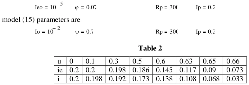
The program Mathcad is being used for calculations. Calculation results are presented in Table 2. In model (14) parameters are

Ieo 105  0.07 Rp 300 Ip 0.2

In model (15) parameters are

Io 102  0.7 Rp 300 Ip 0.2

Table 2

u 0 0.1 0.3 0.5 0.6 0.63 0.65 0.66 ie 0.2 0.2 0.198 0.186 0.145 0.117 0.09 0.073 i 0.2 0.198 0.192 0.173 0.138 0.108 0.068 0.033

Table 2 shows that the calculation results coincide quite well. Better yet, it can be seen if the calculation results are presented graphically. Having mathematical model, it is easy to get model, through which the evolution of capacity changing voltage or current is found. From (15) we will get

P Ip u Io u

2



u

 u

2

Rp



(16)

We will differentiate (16), and reset at zero

uP d

d Ip

2 u

Rp

 Io u

2



u

( )2

 2 Io u

u

 0

(17)

After the evaluation of (17), we get algebraic equation

u332.9 u 244.59u14.7 0 ₍₁₈₎

Third degree algebraic equations have been examined sufficiently. Standard programs were used for the detection of their roots. By taking advantage of one of them we will find that one of equation (18) roots is

u 0 545906

Conclusions

1. 1.When the function exp is used for diode volt-amperes characteristic, then the volt-amperes characteristic of Sun element can not be calculated using standard computer programs. Therefore, special algorithms and programs are developed.

2. If the diode volt-amperes characteristic is described by geometrical progression function of tph, the volt imperial characteristic of Sun element is described by second grade algebraic equation, which solution is easily calculated by an analytical function.

References

Kashif Ishaque n, Zainal Salam, Hamed Taheri Simple, fast and accurate two-diode model for photo voltaic modules Solar Energy Materials & Solar Cells 95 (2011) 586–594. Universiti Technologi Malaysia.

P.T. Boogs, R.H.Byrd, and R.B.Schnabet, “A stable and efficient algorithm for non-liner orthogonal distance regression” SIAM J.Sci.Stat.Comput.,vol.8, no.6, pp.1052-78, 1987.

Donaldas Zanevičius Mathematics without sin α, cos α (When Angle α is Being

Measured in Degrees) and π. International Journal of Applied Science and Technology,

http://www.ijastnet.com/update/index.php/current-issue, Archve Vol.2 No.6 June 2012 Full

Text.