Density-Based Clustering with Constraints
Piotr Lasek1and Jarek Gryz2 1
University of Rzeszow, Poland [email protected]
2 York University, Canada
Abstract. In this paper we present ouric-NBCandic-DBSCANalgorithms for data clustering with constraints. The algorithms are based on density-based clustering algorithmsNBCandDBSCANbut allow users to incorporate background knowl-edge into the process of clustering by means of instance constraints. The knowlknowl-edge about anticipated groups can be applied by specifying the so-calledmust-linkand
cannot-linkrelationships between objects or points. These relationships are then
in-corporated into the clustering process. In the proposed algorithms this is achieved by properly merging resulting clusters and introducing a new notion of deferred points which are temporarily excluded from clustering and assigned to clusters based on their involvement incannot-linkrelationships. To examine the algorithms, we have carried out a number of experiments. We used benchmark data sets and tested the efficiency and quality of the results. We have also measured the efficiency of the algorithms against their original versions. The experiments prove that the introduc-tion of instance constraints improves the quality of both algorithms. The efficiency is only insignificantly reduced and is due to extra computation related to the intro-duced constraints.
Keywords:data mining, data clustering, semi-supervised clustering, clustering with constraints, instance-level constraints
1.
Introduction
Clustering is a well-known and often used data mining technique. Its goal is to assign data objects (or points) to different clusters so that objects that are assigned to the same cluster are more similar to each other than to objects assigned to other clusters [10].
by domain experts. Moreover, in some cases such knowledge can be automatically de-tected. Initially, researchers focused on algorithms that incorporated pairwise constraints on cluster membership or learned distance metrics. Subsequent research was related to algorithms that used many other kinds of domain knowledge [5].
In [12] and [13] we presented the implementation of two neighborhood-based cluster-ing algorithmsic-NBCandic-DBSCAN. These two algorithms combined the well-known
NBC[20] andDBSCAN[8] algorithms with two instance-level constraints,must-linkand
cannot-link. In this paper, we build upon our previous work. In particular, in Section 4,
we provide a formal background behind the algorithms. The standard concepts used in
ic-NBCandic-DBSCAN (e.g.k-neighborhood, dense point, direct neighborhood-based
density reachability, neighborhood-based density reachability, cluster, noise, nearest clus-ter, parent clusclus-ter, etc.) had to be adjusted to the new context of instance constraints and required new definitions. To improve readability, we have introduced a number of exam-ples and figures illustrating the new concepts. Last but not least, we have added an entirely new section with experimental results to verify both quality as well as efficiency of the algorithms.
The paper is divided into six sections. In Section 2 we give a brief introduction to clustering with constraints and describe the related work in the field of constrained clus-tering – especially related to density-based clusclus-tering. In Section 3, the classicDBSCAN
andNBCalgorithms are described. In Section 4 we present our own method. Section 5 contains an experimental evaluation of our algorithms. Conclusions and further research is discussed in Section 6.
2.
Constraints
2.1. Instance-level constraints
In clustering algorithms with constraints, background or expert knowledge can be incor-porated into algorithms by means of different types ofconstraints. [5]. Several types of constraints have been identified so far, for example, instance constraints describing re-lations between objects or distance constraints such as inter–cluster δ–constraints and intra–cluster–constraints [2]. Nevertheless, the hardinstance-levelconstraints seem to be most useful since the incorporation of just few constraints of this type can improve clustering accuracy. (We use the Silhouette score to measure clustering quality in our experiments.)
In [16] authors introduced two kinds ofinstance-levelconstraints, namely: the
must-linkandcannot-linkconstraints. These constraints are simple yet have interesting
prop-erties. For examplemust-linkconstraints are symmetrical, reflexive and transitive: if two points,p0andp1are in amust-linkrelationship, that is,c=(p0, p1)(see Table 1 for
nota-tion), then these points should be assigned to the same cluster. On the other hand, if two pointsr0 andr1 are in acannot-link relationship, that is,c6=(r0, r1), then these points
must not be assigned to the same cluster.
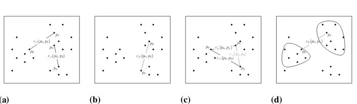
Consider the following example based on Figure 1. In Figure 1.a we present a sample dataset with two must-link constraints c=(p0, p1)and c=(p2, p3). Each pair of points
should be assigned to the same cluster.In Figure 1.b we present a sample dataset with
Table 1.Notation related toinstance-levelconstraints used in the paper and auxiliary variables used in pseudo-code of the algorithm.
Notation Description
C(p) The cluster to which a pointpwas assigned. If a point has not been decided yet to which cluster it should be assigned thenC(p)returnsUNCLASSIFIED. Ifpis anoisepoint, then C(p) =NOISE.
C= The set of pairs of points that are in amust-linkrelation.
c=(p0, p1) Two pointsp0 andp1are in amust-linkrelation (must be assigned to the same resulting cluster).
C=(p) The set of points which are in amust-linkrelation with pointp. C6= The set of pairs of points that are in acannot-linkrelation.
c6=(r0, r1) Two pointsr0andr1are in acannot-linkrelation (must not be assigned to the same resulting cluster).
C6=(r) The set of points which are in acannot-linkrelation with pointr.
ClusterId The auxiliary integer variable used for storing currently-created clusters identifier. p.ClusterId By using such a notation we refer to aClusterIdrelated to pointp.
p.ndf Such a notation is used to refer to a value of theNDFfactor associated with pointp. Rd,Rt The auxiliary variables for storing deferred points.
DP Set The variable for storing dense points. It is used for in an iterative process of assigning points to clusters.
andp1will not be assigned to the same cluster.In Figure 1.c and Figure 1.d we illustrate
basic features of instance constraints such as transitivity, reflexiveness, symmetry as well
as entailment.
2.2. Related Work
In constrained clustering algorithms, background or expert knowledge can be incorpo-rated into algorithms by means of different types of constraints. Over the years, several methods of using constraints in clustering algorithms have been developed [5]. Constraint-based methods proposed so far employ techniques such as modifying the clustering objec-tive function including a penalty for satisfying specified constraints [6], clustering using conditional distributions in an auxiliary space, enforcing all constraints to be satisfied during clustering process [17] or determining clusters and constraints based on neighbor-hoods derived from already available labelled examples [1]. In the distance-based meth-ods, the distance measure is designed so that it satisfies given constraints [11,4]. Among algorithms proposed so far, a few represent modifications of density based algorithms, such asC-DBSCAN[15],DBCCOM[7] orDBCluC[18].
C-DBSCAN[15] is an example of a density-based algorithm usinginstance-level
con-straints where concon-straints are used to dictate whether some points may appear in the same cluster or not. In the first step, the algorithm partitions the dataset into subspaces using the
KD-Tree[3] and then enforcesinstance-levelconstraints within each tree leaf producing
so-calledlocal clusters. Next, undercannot-link constraints, adjacent local clusters are merged enforcingmust-linkconstraints. Finally, adjacent clusters are merged hierarchi-cally enforcing remainingcannot-linkconstraints.
DBCluC[18] which was also based on theDBSCAN [8] employs an obstacle
•p0 •p1
• p3 • p2 • • • • • • • • • • • • • • • •
c=(p0, p1)
c=(p2, p3)
(a) • • • • • • • • • • • • • • • • • • • •p1
c6=(p0, p1) p0 (b) • p0 • p1 •
•p2 • • • • • • • • • • • • • • • •
c=(p0, p1)
c=(p2, p3)
c=(p2, p3)
(c)
•p0 •p1
• • • • • • • • • • • • • • • • • •
c6=(p0, p1)
(d)
Fig. 1.An illustration of (a)must-linkconstraints connecting pointsp0andp1as well as p2andp3. Points that are connected by must-link constraint have to be assigned to the
same cluster; (b)cannot-linkconstraint connecting pointsp1andp2. In spite of the fact
that points may be located relatively closely, if there is acannot-linkrelation between them, they cannot by assigned to the same cluster; (c) transitive, reflexive and symmetrical features ofmust-linkconstraints.p0andp1as well asp0andp2are
connected bymust-linkconstraints, thusp1andp2are also connected by amust-link
constraint; (d) entailedcannot-linkconstraints. All points from clusterss0ands1cannot
be assigned to the same cluster because ofc6=(p0, p1)constraint
is leveraged by a reduction of polygons modelling the obstacles – the algorithm simply removes unnecessary edges from the polygons making the clustering faster in terms of number of constraints to be analysed. Nevertheless, the mechanism of obstacle reduction requires a complex preprocessing to be done before clustering.
TheDBCCOMalgorithm [7] pre-processes an input dataset by modeling the presence
of physical obstacles - similarly toDBCluC. It also detects clusters of arbitrary shapes and size and is also considered to be insensitive to noise as well as an order of points in a dataset. The algorithm comprises of three steps: first, it reduces the obstacles by employing the edge reduction method, then performs the clustering and finally applies hierarchical clustering on formed clusters. The obstacles in the algorithm are represented as simple polygons and however the algorithm uses a more efficient polygon edge reduc-tion algorithm thanDBCluC. The results reported by the authors algorithm confirm that it can perform polygon reduction even faster thanDBCCOMand can produce a hierarchy of clusters.
3.
Density-based clustering
Density-based clustering algorithms use density functions to identify clusters. Clusters are dense regions separated by regions of empty space or low density called noise or outliers. Clusters generated in this way can be of arbitrary shape. In this section we describe two density-based algorithms:DBSCANandNBC.
3.1. DBSCAN
TheDBSCANalgorithm [8] is a well known density-based clustering algorithm. The
neighborhood,M inP ts – the minimal number of points within -neighborhood. Each point inDhas an attribute calledClusterIdwhich stores the cluster’s identifier and ini-tially is equal toUNCLASSIFIED. The key definitions related to theDBSCANalgorithm shown below will be used in the sequel. Again, the general notation is given in Table 1.
Definition 1 (–neighborhood, orN N(p)of pointp).–neighborhood of pointpis the
set of all pointsqin datasetDthat are distant frompby no more than; that is,
N N(p) ={q∈D|dist(p, q)≤},
wheredistis a distance function.
Clusters inDBSCANare associated with core points which can be considered as seeds of clusters.
Definition 2 (core point).pis acore pointwith respect toif its-neighborhood contains
at leastM inP tspoint; that is,|N N(p)| ≥M inP ts.
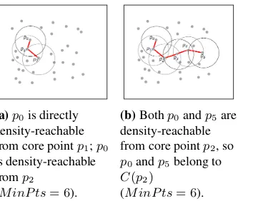
The pointp2in Figure 3a is a core point as its–neighborhood contains 6 points (we
assumeM inP ts= 6in this case).
Definition 3 (directly density-reachable points).Pointpis directly density reachable
from pointqwith respect toandM inP tsif the following two conditions are satisfied:
a) p∈N N(q)
b) qis a core point.
Figure 3a illustrates the concept of direct reachability.
Definition 4 (density-reachable points).Pointpis density-reachable from a pointqwith
respect to and M inP tsif there is a sequence of points p1, ..., pn such thatp1 = q,
pn=pandpi+1and is directly density-reachable frompi,i= 1. . . n−1.
Figure 3b illustrates the concept of reachability.
Definition 5 (cluster).A cluster is a non-empty set of points inD which are
density-reachable from the same core point.
Although Definition 5 is formulated somewhat differently than the definition provided in [8], the resulting clusters are identical in both cases.
Points that are not in dense areas are not associated with any clusters and are consid-ered noise.
Definition 6 (noise).Noise is the set of all points in D that are not density-reachable
from any core point.
DBSCAN proceeds as follows. Firstly, the algorithm generates a label for the first
(a) (b) (c) (d)
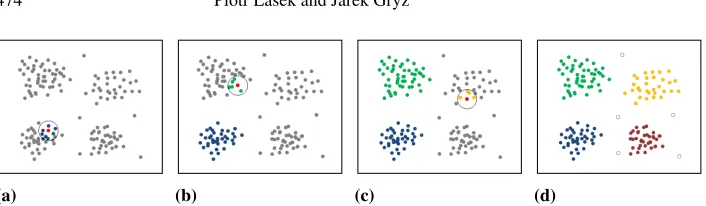
Fig. 2.Illustration of a sample execution of theDBSCANalgorithm. The neighborhood
of the first core point is assigned to a cluster (a). Subsequent assignment of density-reachable points forms the first cluster; initial seeds are determined for the second cluster (b). The second cluster reaches its maximum size; the initial seeds are determined for the third cluster (c). The third cluster reaches its maximum size; the initial seeds are determined for the fourth cluster. Finally,DBSCANlabels noise points represented here by empty dots (d).
after point, it may happen that theClusterIdattributes of some points may change be-fore these points are actually analyzed. Such a case may occur when a point is density-reachable from a core point examined earlier. Such density-density-reachable points will be as-signed to the cluster of a core point and will not be analyzed later. If a currently ana-lyzed pointphas not been classified yet (the value of itsClusterIdattribute is equal to
UNCLASSIFIED), then theExpandClusterfunction is called for this point. Ifpis a core point, then all points inC(p)are assigned by theExpandClusterfunction to the cluster with a label equal to the currently created cluster’s label. Next, a new cluster label is gen-erated byDBSCAN. Otherwise, ifpis not a core point, the attributeClusterIdof pointp
is set toNOISE, which means that pointpwill be tentatively treated as noise. After ana-lyzing all points inD, each point’s attributeClusterIdstores a respective cluster label or its value is equal toNOISE. An illustration of a sample execution ofDBSCANhas been ploted in Figure 2.
3.2. Neighborhood-based clustering
The Neighborhood-Based Clustering (NBC) [20] algorithm also belongs to the class of density based clustering algorithms. The characteristic feature ofNBCcompared to DB-SCANis its ability to measure relative local densities. Hence, it is capable of discovering clusters of different local densities and of arbitrary shape. The algorithm has two param-eters: the set of pointsDand the numberkwhich is used to describe density of a point.
The key definitions related to theNBCalgorithm are presented below;k–neighborhood andk+–neighborhood, defined below, are parameters used to describe dense
neighbor-hoods.
Definition 7 (k–neighborhood, orkN N(p)).k–neighborhood of pointpis a set ofk
(k >0) points satisfying the following conditions:
|kN N(p)|=k, and
Definition 8 (k+–neighborhood, ork+N N(p)).k+–neighborhood of pointpis equal to0N N(p)where:
0=max({dist(p, v)|v∈kN N(p)}).
k+–neighborhood is similar toN N(p)(see Def. 3.1). However,is not a parameter
given a priori to the algorithm, but a property of dense neighborhoods relative to a given data set.
Definition 9 (punctured k+–neighborhood). Puncturedk+–neighborhood of point p
k+N N(p−)is equal tok+N N(p)
\ {p}; that is:
k+N N(p−) =k+N N(p)\ {p}.
The concept ofk+–neighborhood ofpis illustrated in Figure 4a.
Definition 10 (reversed punctured k+–neighborhood of a point p). Reversed
punc-turedk+–neighborhood of a pointp Rk+N N(p)is the set of all pointsq6=pin dataset
Dsuch thatp∈k+N N(q−); that is:
Rk+N N(p) ={q∈D|p∈k+N N(q−)}.
(a)p0is directly
density-reachable from core pointp1;p0
is density-reachable fromp2
(M inP ts= 6).
(b)Bothp0andp5are
density-reachable from core pointp2, so
p0andp5belong to
C(p2)
(M inP ts= 6).
Fig. 3.Illustration of some of the concepts
ofDBSCAN
(a)q6is directly
neighborhood-based density reachable frompbecause
q6∈k+N N(p−).
(b)Pointq12is
neighborhood-based density reachable from pointq3.
Fig. 4.Illustration of some of the concepts ofNBCalgorithm.
Definition 11 (neighborhood-based density factor of a point –N DF(p)).
Neighbor-hood-based density factor of a pointpis defined as
N DF(p) =|Rk+N N(p)|/|k+N N(p−)|.
Points having the value of the value ofN DF factor equal to or greater than 1, are
considereddense.
Definition 12 (dense point).Pointpis called alocal dense pointif itsN DF(p)is greater
Definition 13 (directly neighborhood–based density reachable).A pointpis directly
neighborhood–based density reachable from pointqifp∈k+N N(q−)andqis a dense
(core) point.
Pointq6in Figure 4a is directly neighborhood–based density reachable from pointp.
Definition 14 (neighborhood-based density reachable). A pointp is
neighbor-hood-based density reachable from r if pis directly neighborhood-based density reachable
fromqandris directly neighborhood-based density reachable fromq.
Pointq12in Figure 4b is directly neighborhood–based density reachable from pointq3.
Definition 15 (cluster).A cluster is a maximal non-empty subset ofDsuch that for two
pointspandqin the cluster,pandqare neighborhood-based density-reachable from a
local core point with respect tok, and ifpbelongs to clusterCandqis
neighborhood-based density connected withpwith respect tok, thenqbelongs toC.
Definition 16 (noise).Noise is the set of all points inDthat do not belong to any cluster.
In other words, noise is the set of all points inDthat are not neighborhood-based
density-reachable from any local core point.
In order to find clusters,N BC starts with calculating values of NDF factors for each pointpiin a databaseD,i= 0,1, . . . ,|D|. Next, for eachpi, a value of NDF is checked.
If it is greater than or equal to 1, thenpi is assigned to the currently created clusterc
(identified by the value ofClusterId). Next, the temporary variableDP Set for stor-ing references to points, is cleared and each point, say q, belonging to k+N N(p−
i ) is
assigned to c. If q.ndf is greater than or equal to 1, then q is also added toDP Set. Otherwise,qis omitted and a next point fromk+N N(p−
i )is analyzed. Further, for each
point fromDP Set, sayr,k+N N(r−)is computed. All unclassified points belonging tok+N N(r−)are assigned tocand points having values of NDF greater than or equal to 1 are added toDP Set. Next,r is removed fromDP Set. When DP Setis empty,
ClusterIdis incremented and a next point fromD, namelypi+1, is analyzed. Finally,
if there are no more points inD having values ofN DF factor greater than or equal to
1, then all unclassified points inD are marked as N OISE.
4.
Clustering with Constraints
In this section we present two density-based algorithms with constraints based on
DBSCAN and NBC. The main modification in both algorithms is the introduction
of the DEFERRED points. The deferred points are in –neighborhood (for DBSCAN
algorithm) or k+–punctured neighborhood (for the NBC algorithm) of points
in-volved in cannot-link relationship. The original algorithms are then first executed without the deferred points after which the points are assigned to appropriate clusters to satisfy their cannot-link constraints.
Themust-linkconstraints are handled in a simple way. In the original algorithms, the
to the cluster originating inp. In this way, the algorithm can connect two remote regions via a bridge defined by the pair of points in amust-linkrelationship.
Our interpretation of the instance constraints is slightly different from most of the ex-isting approaches which stop execution of the clustering algorithms upon the discovery of conflicting constraints. We believe that instance constraints do not necessarily have to be fully satisfied. ic-NBC andic-DBSCAN use techniques similar to DBCluC [18] where the concept of so-calledobstacle pointswas introduced. Obstacle points are ig-nored during the process of clustering. In our algorithms, we treatcannot-linkconstraints (along with theirnearest neighbors) as points which constitute similarobstacles, but we do not ignore them completely during clustering
Thus, in the process of clustering, if a conflicting constraints exists, the algorithm does not have to be stopped, and conflicting points are labeled asNOISE.
4.1. ic-DBSCAN
In this subsection we offer a modified version ofDBSCANwith constraints. First we intro-duce a definition ofdeferredpoints (Definition 17) and then present modified definitions
of clusterandnoise- Definition 18 and Definition 21, respectively.
Definition 17 (deferred point).A pointpis calleddeferredif it is in acannot-link
rela-tionship with any other point or it belongs to a–neighborhoodN N(q), whereqis any
point in acannot-linkrelationship (q∈C6=). In the latter case we callqa parent point.
Definition 18 (cluster).A cluster is a maximal non-empty subset ofDsuch that:
– for twonon-deferredpointspandqin the cluster,pandqare neighborhood-based
density-reachable from a local core point with respect tok, and ifpbelongs to cluster
Candqis also neighborhood-based density connected withpwith respect tok, then
qbelongs toC;
– adeferredpointpis assigned to a clusterCif the 1st-nearest punctured neighbour of
pbelongs toC(1−N N(p−)∈C), otherwise,pis considered as a noise point.
Definition 19 (nearest cluster).A nearest cluster of a given point pis a clusterC to
whichpbelongs.
Definition 20 (parent cluster).A parent cluster of a given pointp(gp) is a clusterCto
which a parent point ofpbelongs.
Definition 21 (noise).The noise is the set of all points inDsuch that each of them is:
– not density-reachable from any core point or
– is adeferredpoint that has two or more neighbours at the same distance from it and thus can not be unambiguously assigned to a cluster.
In other words,noiseis the set of all points inD that are not neighborhood-based
density-reachable from any localcore pointanddeferredpoints points that could not be
assigned to any cluster.
In the first phase,ic-DBSCAN algorithm (Figure 6a) omits all points which are in-volved in any cannot-link relationship and marks them as DEFERRED. Then, it adds those points to an auxiliary list calledRd which will be later used in the main loop of
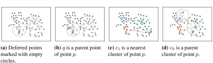
r
q
(a)Deferred points marked with empty circles.
p r
q
(b)qis a parent point of pointp.
p c1
c2 c0
(c)c1is a nearest
cluster of pointp.
p c1
c2 c0
q r
(d)c0is a parent
cluster of pointp.
Fig. 5.An illustration of definitions of deferred points (a), parent point (b), nearest and parent cluster (c,d).
Then the algorithm iterates through allUNCLASSIFIEDpoints fromDexcept those which were added toRd. For all of those points it calls theExpandClusterfunction (Figure
6c) and passes all necessary parameters. The main modifications of theExpandCluster
function (compared to the classicDBSCANalgorithm) is in how themust-linkconstraints are processed. When amust-linkpoint is processed and it is acore pointor belongs to a neighbourhood of a point which is acore point, then it is assigned toseedsorcurSeeds
lists (containingseed points) depending on which part of theExpandClusterfunction is currently executed. ( TheseedsandcurSeedsare lists containing of points that belong to–neighborhoods of currently processed point in theExpandClusterfunction and the number of points in the neighborhood is greater or equal toM inP ts.)
The last part of the algorithm is to process the set ofDEFERREDpoints. This is done by means of the AssignDeferredPointsfunction (Figure 6b). For each pointqfromRd
(a list of points which were marked asDEFERREDin the main algorithm method) the function determines what would be the parent clustergpof q. Next, it finds a pointp6=
involved incannot-linkrelationship and similarly determines its parent clustergp6=. Then,
if those two parent clusters are the same (gp = gp6=) the DEFERREDpoint q cannot
be assigned to the nearest clustergp and is labeled asNOISE. Otherwise, if two
par-ent clusters are differpar-ent q is assigned to gp.
4.2. ic-NBC
In this subsection we offer our new neighborhood-based constrained clustering algorithm calledic-NBC. The algorithm is based on theNBCalgorithm [20] but uses bothmust-link
andcannot-linkconstraints for incorporating knowledge into the algorithm.
Below we present the definition of deferred point as well as modified definitions of cluster and noise - Definition 23 and Definition 24, respectively.
The ic-NBC algorithm employs the same definitions as NBC which are used
in a process of clustering to assign points to appropriate clusters or mark them as noise. In NBC three types of points can be distinguished: unclassified,
classi-fied and noise points. In ic-NBC, we also employ a concept of DEFERRED points
although defined slightly different than before.
Definition 22 (deferred point).A pointpis deferred if it is involved in acannot-link
rela-tionship with any other point or it belongs to ak+–punctured neighborhoodk+N N(q−),
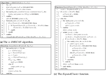
Algorihtmic-DBSCAN(D,k,C=,C6=)
Rd=∅ 1.
label all points inDasUNCLASSIFIED; 2.
ClusterId= label of a first cluster; 3.
for eachpointqinvolved in any constraint fromC6=do
4.
labelqand points inN N(q) asDEFERRED; 5.
endfor;
6.
add allDEFERREDpoints toRd; 7.
foreachpointpin setD\Rddo
8.
if(p.ClusterId=UNCLASSIFIED)then
9.
ifExpandCluster(D,p,ClusterId,,M inP ts)then
10.
ClusterId=NextId(ClusterId); 11. endif; 12. endif; 13. endfor; 14.
AssignDefferedPoints(D,p,ClId,M inP ts,,C=,C6=);
15.
(a)Theic-DBSCANalgorithm.
FunctionAssignDeferredPoints(D,Rd,C6=)
for eachpointq∈Rddo
1.
p←GetParent(q); 2.
gp←NearestCluster(p); 3.
p6=←C6=(p);
4.
gp6==NearestCluster(p6=);
5.
ifgp=gp6=then
6.
markqasNOISE;
7.
else if
8.
assign pointqtogp; 9.
end if;
10.
removeqfromRd; 11.
end for;
12.
(b)Assigning deferred points to clusters.
FunctionExpandCluster(D,p,ClId,M inP ts,,C=,C6=)
seeds=Neighborhood(D,p,); 1.
if|seeds|< M inP tsthen
2.
p.ClusterId=NOISE; 3.
returnFALSE;
4.
else do
5.
for eachpointqinseedsdo
6.
q.ClusterId=ClId; 7.
addC=(q) toseeds;
8.
endfor
9.
deletepfromseeds; 10.
while|seeds|>0do
11.
curP oint= first point inseeds; 12.
curSeeds=Neighborhood(D,curP oint,); 13.
if|curSeeds| ≥M inP tsthen
14.
for eachpointqincurSeedsdo
15.
addC=(q) toseeds;
16.
ifq.ClusterId=UNCLASSIFIEDthen
17.
q.ClusterId=ClId; 18.
appendqtoseeds; 19.
else ifq.ClusterId=NOISEthen
20.
q.ClusterId=ClId; 21. end if; 22. end for; 23. end if; 24.
deletecurP ointfromseeds; 25.
end while;
26.
end else;
27.
(c)TheExpandClusterfunction.
Fig. 6.The pseudo-code of theic-DBSCANalgorithm using instance constraints.
Definition 23 (cluster).A cluster is a maximal non-empty subset ofDsuch that:
– for twonon-deferredpointspandqin the cluster,pandqare neighborhood-based
density-reachable from a local core point with respect tok, and ifpbelongs to cluster
Candqis also neighborhood-based density connected withpwith respect tok, then
qbelongs toC;
– adeferredpointpis assigned to a clusterCif the nearest neighbour ofpwhich is not incannot-linkrelationship withpbelongs toC, otherwisepis considered as a noise point.
Definition 24 (noise).Noise is the set of all points inDthat:
– have not been assigned to any cluster or
– each of them is a deferred pointpwhose1+N N(p−)neighborhood contains points
assigned to different clusters and thus can not be unambiguously assigned to a par-ticular cluster.
In other words, noise is the set of all points inDthat are not neighborhood-based
density-reachable from any local core point anddefferedpoints points which could be assigned
to two or more clusters.
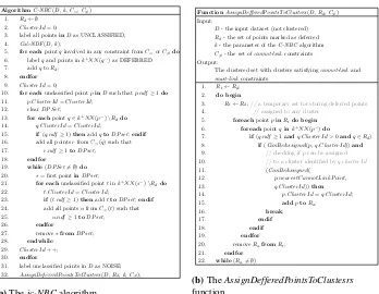
ic-NBC(Figure 7a) can be divided into two main steps. In the first step the algorithm
AlgorithmC-NBC(D,k,C=,C6=)
Rd← ∅
1.
ClusterId= 0;
2.
label all pointsinDas UNCLASSIFIED;
3.
CalcNDF(D,k); 4.
for eachpointqinvolved in any constraint fromC=orC6=do
5.
labelqand points ink+N N(q−) as DEFERRED
6.
addqtoRd; 7.
endfor
8.
ClusterId= 0;
9.
for eachunclassified pointpinDsuch thatp.ndf≥1do
10.
p.ClusterId=ClusterId;
11.
clearDP Set; 12.
for eachpointq∈k+N N(p−)\Rddo 13.
q.ClusterId=ClusterId;
14.
if(q.ndf≥1)thenaddqtoDP set;endif
15.
add all pointsrfromC=(q) such that
16.
r.ndf≥1toDP set;
17.
endfor
18.
while(DP Set6=∅)do
19.
s= first pointinDP set; 20.
for eachunclassified pointtink+N N(s−)\Rddo 21.
t.ClusterId=ClusterId;
22.
if(t.ndf≥1)thenaddttoDP set;endif
23.
add all pointsufromC=(t) such that
24.
u.ndf≥1toDP set;
25.
endfor
26.
removesfromDP set;
27.
endwhile
28.
ClusterId+ +;
29.
endfor
30.
label unclassified points inDas NOISE;
31.
AssignDeferredPointsToClusters(D,Rd,k,C6=);
32.
(a)Theic-NBCalgorithm.
FunctionAssignDefferedPointsToClusters(D,Rd,C6=)
Input:
D- the input dataset (not clustered)
Rd- the set of points marked as deferred k- the parameter of theC-NBCalgorithm
C6=- the set ofcannot-linkconstraints
Output:
The clustered set with clusters satisfyingcannot-linkand
must-linkconstraints.
Rt←Rd; 1.
do begin
2.
Rt←Rd;// a temporary set for storing deferred points 3.
// assigned to any cluster 4.
foreachpointpinRtdo begin
5.
foreachpointqink+N N(p−)do
6.
if(q.ndf≥1andq.ClusterId >0andq∈Rd) 7.
if(CanBeAssigned(p,q.ClusterId))and
8.
// checking ifpcan be assigned 9.
// to a cluster identified byq.clusterId
10.
(CanBeAssigned( 11.
p.nearestCannotLinkP oint, 12.
q.ClusterId))then
13.
p.ClusterId=q.ClusterId; 14.
addptoRa;
15. break; 16. endif 17. endif 18. endfor 19.
removeRafromRt; 20.
endfor
21.
while(Ra6=∅)
22.
(b)TheAssignDefferedPointsToClustesrs
function.
Fig. 7.The pseudo-code of theic-NBCalgorithm.
– determines which points will be considered asDEFERRED;
– excludes these points from all calculations (except to compute the values ofN DF
factors); and
– merges areas of clustered dataset according tomust-linkconstraints.
Theic-NBCalgorithm starts with theCalcNDFfunction. After calculating the NDF
factors for each point fromD, the deferred points are determined by scanning pairs of
cannot-linkconnected points. These points are added to an auxiliary setRd.
Then, the clustering process is performed in the following way: for each pointpwhich was not marked asDEFERRED, it is checked ifp.ndf is less than 1. Ifp.ndf <1, then
pis omitted and a next fromDP Setis checked. Ifp.ndf ≥1, thenpas adense pointis assigned to the currently-created cluster identified by the current value ofClusterId.
Next, the temporary variableDP Setis cleared and each non-deferred point, say q, belonging tok+N N(p−)\R
dis assigned to the currently-created cluster identified by the
current value of theClusterIdvariable. Additionally, ifq.ndf≥1, then it is assigned to
DP Setas well as all dense points which are in a must-link relation withq.
Next, for each unclassified point fromDP Set, says, its puncturedk+–neighborhood
is determined. Each point, sayt, which belongs to this neighborhood and has not been labeled as deferred yet is assigned to the currently created cluster and if its value ofN DF
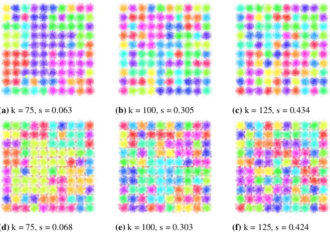
(a)k = 75, s = 0.063 (b)k = 100, s = 0.305 (c)k = 125, s = 0.434
(d)k = 75, s = 0.068 (e)k = 100, s = 0.303 (f)k = 125, s = 0.424
Fig. 8.Results of clustering for the Birch1 dataset usingNBC(a-c), andic-NBC(d-f). Colors represent mined clusters.kis a parameter if the algorithm. sis a value of the Silhouette factor computed for the given clustering result. Red dashed lines denote
cannot-linkconstraints.
and next point fromDP Setis processed. WhenDP Setis emptied, thenClusterIdis incremented. After all points fromD are processed, unclassified points are marked as noise by setting the values of theirClusterIdattribute toNOISE. However, in order to process the deferred points, theAssignDeferredPointsToClusterfunction is invoked. The function performs so that for each deferred pointpit finds the nearest pointqassigned to any cluster and checks whether it is possible (in accordance with cannot-link constraints) to assignpto the same cluster asq. Additionally, the function checks if the assignment of
pto a specific cluster will not violate previous assignments of deferred points.
5.
Experiments
In this section we present results of the experiments we performed to test the quality and efficiency of the proposed methods. We divided the experiments into two parts. First we focused on qualityof clustering, then on the efficiency.
Datasets. For the experiments we used three standard two dimensional clustering
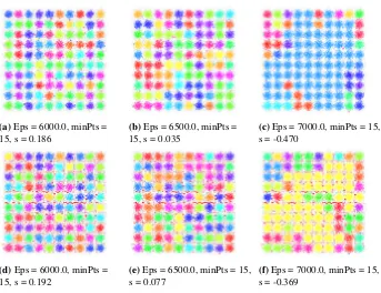
(a)Eps = 6000.0, minPts = 15, s = 0.186
(b)Eps = 6500.0, minPts = 15, s = 0.035
(c)Eps = 7000.0, minPts = 15, s = -0.470
(d)Eps = 6000.0, minPts = 15, s = 0.192
(e)Eps = 6500.0, minPts = 15, s = 0.077
(f)Eps = 7000.0, minPts = 15, s = -0.369
Fig. 9.Results of clustering for the Birch1 dataset usingDBSCAN(a-c), andic-DBSCAN
(d-f). Colors represent mined clusters.EpsandminP tsare parameters of the algorithm.
(a)k = 900, s = 0.724
(b)k = 950, s = 0.456
(c)k = 1000, s = -1.000
(d)k = 900, s = 0.739
(e)k = 950, s = 0.683
(f)k = 1000, s = 0.346
Fig. 10.Results of clustering for the Birch2 dataset usingNBC(a-c), andic-NBC(d-f). Colors represent mined clusters.kis a parameter if the algorithm. sis a value of the Silhouette factor computed for the given clustering result. Red dashed lines denotecannot-linkconstraints.
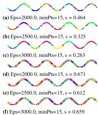
(a)Eps=2000.0, minPts=15, s = 0.464
(b)Eps=2500.0, minPts=15, s = 0.325
(c)Eps=3000.0, minPts=15, s = 0.263
(d)Eps=2000.0, minPts=15, s = 0.671
(e)Eps=2500.0, minPts=15, s = 0.612
(f)Eps=3000.0, minPts=15, s = 0.659
Fig. 11.Results of clustering for the Birch2 dataset usingDBSCAN(a-c), and
ic-DBSCAN(d-f). Colors represent mined
clusters.EpsandminP tsare parameters of the algorithm. sis a value of the Silhouette factor computed for the given clustering result. Red dashed lines denote
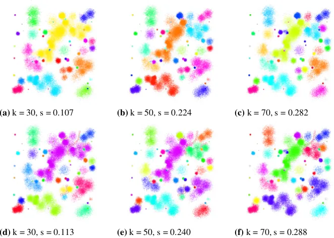
(a)k = 30, s = 0.107 (b)k = 50, s = 0.224 (c)k = 70, s = 0.282
(d)k = 30, s = 0.113 (e)k = 50, s = 0.240 (f)k = 70, s = 0.288
Fig. 12.Results of clustering for the Birch3 dataset usingNBC(a-c), andic-NBC(d-f). Colors represent mined clusters.kis a parameter if the algorithm. sis a value of the Silhouette factor computed for the given clustering result. Red dashed lines denote
cannot-linkconstraints. Black solid lines aremust-linkconstraints. In the experiment 12
(a)Eps = 5000.0, minPts = 15, s = 0.128
(b)Eps = 6000.0, minPts = 15, s = 0.146
(c)Eps = 7000.0, minPts = 15, s = 0.031
(d)Eps = 5000.0, minPts = 15, s = 0.154
(e)Eps = 6000.0, minPts = 15, s = 0.194
(f)Eps = 7000.0, minPts = 15, s = 0.171
Fig. 13.Results of clustering for the Birch3 dataset usingDBSCAN(a-c), and
ic-DBSCAN(d-f). Colors represent mined clusters.EpsandminP tsare parameters of
the algorithm. sis a value of the Silhouette factor computed for the given clustering result. Red dashed lines denotecannot-linkconstraints. Black solid lines aremust-link
constraints. In the experiment 12must-linkand 43cannot-linkconstraints were used.
0 20 40 60 80 100
0 50 100 150 200 250
The ic-DBSCAN runtimes
Birch1 Birch2 Birch3
Number of constraints
T
im
e
[s
ec
.]
(a)ic-DBSCAN.
0 20 40 60 80 100
40 50 60 70 80 90 100
The ic-NBC runtimes
Birch1 Birch2 Birch3
Number of constraints
T
im
e
[s
ec
.]
(b)ic-NBC.
Fig. 14.Charts with the results of experiments for testing efficiency ofic-DBSCAN(a)
Table 2.Results of exeriments. Def - number of deferred points; Count - number of discovered clusters; Silh. - a value of the Silhouette score; Ind. - time of index building; Clust. - time of clustering; Tot. = Ind. + Clust. Times are given in milliseconds.
Data Alg. Param. Ind. Clus. Def. Cnt. Tot. Silh. birch1 NBC 75 10145 63372 47 73517 0.063 birch1 ic-NBC 75 9006 67731 6537 49 76737 0.068 birch1 NBC 100 8980 61405 72 70385 0.305 birch1 ic-NBC 100 10399 74341 9877 73 84740 0.303 birch1 NBC 125 8934 67587 89 76521 0.434 birch1 ic-NBC 125 8791 80985 13542 89 89776 0.424 birch1 DBSCAN 6000.0, 15 9892 29946 223 39838 0.186 birch1 ic-DBSCAN 6000.0, 15 8879 34089 4518 216 42968 0.192 birch1 DBSCAN 6500.0, 15 9702 30969 152 40671 0.035 birch1 ic-DBSCAN 6500.0, 15 8885 34726 5386 146 43611 0.077 birch1 DBSCAN 7000.0, 15 9323 31151 73 40474 -0.470 birch1 ic-DBSCAN 7000.0, 15 9648 37155 6778 74 46803 -0.369 birch2 NBC 900 8955 108149 99 117104 0.724 birch2 ic-NBC 900 9260 187205 77742 100 196465 0.739 birch2 NBC 950 9011 118442 64 127453 0.456 birch2 ic-NBC 950 10281 210245 88899 92 220526 0.683 birch2 NBC 1000 9446 120449 1 129895 -1.000 birch2 ic-NBC 1000 9402 205044 87771 43 214446 0.346 birch2 DBSCAN 2000.0, 15 9370 46691 63 56061 0.464 birch2 ic-DBSCAN 2000.0, 15 9026 68285 26811 89 77311 0.671 birch2 DBSCAN 2500.0, 15 8807 51681 46 60488 0.325 birch2 ic-DBSCAN 2500.0, 15 9470 98568 55157 82 108038 0.612 birch2 DBSCAN 3000.0, 15 9243 56087 39 65330 0.263 birch2 ic-DBSCAN 3000.0, 15 8991 144539 101349 85 153530 0.659 birch3 NBC 30 9093 71470 52 80563 0.111 birch3 ic-NBC 30 8848 72752 213 48 81600 0.090 birch3 NBC 50 8712 78941 54 87653 0.234 birch3 ic-NBC 50 9984 79111 450 50 89095 0.149 birch3 NBC 70 8871 84654 50 93525 0.282 birch3 ic-NBC 70 10469 101585 622 45 112054 0.199 birch3 DBSCAN 5000.0, 15 9132 61933 118 71065 0.133 birch3 ic-DBSCAN 5000.0, 15 8482 63644 247 111 72126 -0.014 birch3 DBSCAN 6000.0, 15 9136 62968 80 72104 0.153 birch3 ic-DBSCAN 6000.0, 15 8644 72144 316 78 80788 0.020 birch3 DBSCAN 7000.0, 15 9293 67478 57 76771 0.031 birch3 ic-DBSCAN 7000.0, 15 8464 72594 515 57 81058 0.069
(a)Results of experiments designed to examine quality of proposed constrained algorithms compared to the original versions of the algorithms using the Silhouette score.
Data Alg. Param. Cons. Cnt. Ind. Clus. Def. Tot. birch1 ic-NBC 100 10 62 8728 63990 359 73077 birch1 ic-NBC 100 20 55 9915 68614 803 79332 birch1 ic-NBC 100 40 39 9089 70127 1544 80760 birch1 ic-NBC 100 60 27 8896 65691 2054 76641 birch1 ic-NBC 100 80 15 9184 65275 2396 76855 birch1 ic-NBC 100 100 10 9746 66166 2661 78573 birch1 ic-DBSCAN 5000.0, 15 10 337 9319 28958 309 38586 birch1 ic-DBSCAN 5000.0, 15 20 337 9520 30872 712 41104 birch1 ic-DBSCAN 5000.0, 15 40 333 8739 29988 1192 39919 birch1 ic-DBSCAN 5000.0, 15 60 335 10501 31883 2002 44386 birch1 ic-DBSCAN 5000.0, 15 80 332 8738 31548 2533 42819 birch1 ic-DBSCAN 5000.0, 15 100 328 8960 31973 3216 44149 birch2 ic-NBC 50 10 92 9041 50207 117 59365 birch2 ic-NBC 50 20 81 8966 51558 237 60761 birch2 ic-NBC 50 40 65 10092 55825 633 66550 birch2 ic-NBC 50 60 49 8889 51154 708 60751 birch2 ic-NBC 50 80 32 9199 55838 942 65979 birch2 ic-NBC 50 100 22 9600 56700 1135 67435 birch2 ic-DBSCAN 1000.0, 15 10 94 9652 41497 3836 54985 birch2 ic-DBSCAN 1000.0, 15 20 82 11627 49121 6593 67341 birch2 ic-DBSCAN 1000.0, 15 40 68 9514 44713 12791 67018 birch2 ic-DBSCAN 1000.0, 15 60 53 9078 49770 18159 77007 birch2 ic-DBSCAN 1000.0, 15 80 36 9360 56373 24097 89830 birch2 ic-DBSCAN 1000.0, 15 100 39 9150 56351 26937 92438 birch3 ic-NBC 50 10 45 9050 81492 171 90713 birch3 ic-NBC 50 20 36 9494 80983 421 90898 birch3 ic-NBC 50 40 29 9165 81561 643 91369 birch3 ic-NBC 50 60 22 8499 80386 1097 89982 birch3 ic-NBC 50 80 15 10239 83934 1196 95369 birch3 ic-NBC 50 100 16 9206 83578 1627 94411 birch3 ic-DBSCAN 6000.0, 15 10 72 8711 90199 32349 131259 birch3 ic-DBSCAN 6000.0, 15 20 67 8621 90319 41090 140030 birch3 ic-DBSCAN 6000.0, 15 40 65 8433 91516 40586 140535 birch3 ic-DBSCAN 6000.0, 15 60 61 8815 109920 67327 186062 birch3 ic-DBSCAN 6000.0, 15 80 62 8760 107802 65545 182107 birch3 ic-DBSCAN 6000.0, 15 100 58 9075 124772 80327 214174
Implementation. Both implementations of the algorithms employ the same in-dex structure – the R-Tree [9]. We implemented them in Java and performed the experiments on MacBook Pro 2.8GHz eight-core Intel Core i7, 16GB RAM. The source code can be found under the following link: http://github. com/piotrlasek/clustering
Quality. To examine how quality of clustering could be improved by means of instance
constraints, we used the Silhouette score [14], a method of interpretation and validation of consistency within clusters. TheSilhouette scorefor a pointiis given by the follow-ing formulas(i) = max(b(i){a(i),b(i)−a(i))}, where a(i)is the avarage dissimilarity of i with all other points within the same cluster,b(i)is the lowest average dissimilarity ofito any other cluster to whichi does not belong. The silhouette value measurescohesion and
separationthat means of how similar an object is to its own cluster compared to other
cluster. The values of the silhouette score can range from −1 to +1, where a higher value indicates that the object was correctly assigned to its cluster. We report the mean Silhouette value over all objects in a dataset. Times and values of the Silhouette score are reported in Table 2a and Figures 8-14.
The introduction of instance constraints improves the quality of bothDBSCANas well asNBC; in most cases, the improvement is substantial. However, the clustering quality rises much more forDBSCAN than forNBC.NBCis designed - contrary toDBSCAN
- to discover clusters with varying local densities (thanks to how the N DF factor was defined). In other words,DBSCAN mines clusters based on a global notion of density,
NBCdetermines clusters using density calculated locally. For this reason, we do not see as much improvement in employing constraints inNBCcompared toDBSCAN.
Efficiency. In the second part of the experiments we focused on time efficiency
of clustering with respect to the number of constraints as well as values of algo-rithms’ parameters (Table 2b, Figures 14a-b).
When performing experiments usingic-NBCwe were changing the number of
must-link andcannot-link constraints from 10to 100. Since the additional operations must
have been be performed in order to take the constraints into account, this was obvious that constrained versions of the algorithms had to be less effective than the original ones. However, as plotted in Figures 14a-b, the algorithms’ execution times are almost con-stant with respect to the number of constraints used.
6.
Conclusions
In this paper we have presented two clustering algorithms with constraints, ic-NBC
and ic-DBSCAN, which were designed to let users introduce instance constraints
for specifying background knowledge about the anticipated groups. In our approach we treat must-link constraints as more important than cannot-link constraints. Thus, we try to satisfy all must-link constraints (assuming, of course, that all of them are valid) before incorporating any cannot-link constraints. When processing cannot-link
constraints, points which are contradictory (in terms of satisfying both must-link
and cannot-link constraints) are marked as noise.
The experiments proved that the introduction of instance constraints improved the quality of clustering in both cases. At the same time, due to additional computations needed to process constraints, the performance of the algorithms was reduced but only marginally. The experiments also showed that the number of constraints does not have a critical impact on the algorithms performance.
In this work we have focused on of incorporatinginstance-levelconstraints into clus-tering algorithms by modifying the algorithms. Nevertheless, there are other ways of in-corporating constraints into the process of clustering. For example, the constraints can be used to modify a distance matrix so that it reflectsmust-linkandcannot-linkrelationships. Such a matrix can then be used as an input to the original algorithm without constraints. We believe that this is a promising area of research and we plan to explore it in future.
References
1. Basu, S., Banerjee, A., Mooney, R.: Semi-supervised clustering by seeding. In: In Proceedings of 19th International Conference on Machine Learning (ICML-2002. Citeseer (2002) 2. Basu, S., Davidson, I., Wagstaff, K.: Constrained clustering: Advances in algorithms, theory,
and applications. CRC Press (2008)
3. Bentley, J.L.: Multidimensional binary search trees used for associative searching pp. 509–517 (1975)
4. Chang, H., Yeung, D.Y.: Locally linear metric adaptation for semi-supervised clustering. In: Proceedings of the twenty-first international conference on Machine learning, p. 20. ACM (2004)
5. Davidson, I., Basu, S.: A survey of clustering with instance level constraints. ACM Transac-tions on Knowledge Discovery from Data1, 1–41 (2007)
6. Davidson, I., Ravi, S.: Clustering with constraints: Feasibility issues and the k-means algo-rithm. In: SDM, vol. 5, pp. 201–211. SIAM (2005)
7. Duhan, N., Sharma, A.: Dbccom: Density based clustering with constraints and obstacle mod-eling. In: Contemporary Computing, pp. 212–228. Springer (2011)
8. Ester, M., Kriegel, H.P., Sander, J., Xu, X.: A density-based algorithm for discovering clusters in large spatial databases with noise. In: Kdd, vol. 96, pp. 226–231 (1996)
9. Guttman, A.: R-trees: a dynamic index structure for spatial searching, vol. 14. ACM (1984) 10. Han, J., Kamber, M.: Data Mining, Southeast Asia Edition: Concepts and Techniques. Morgan
kaufmann (2006)
11. Hertz, T., Bar-Hillel, A., Weinshall, D.: Boosting margin based distance functions for cluster-ing. In: Proceedings of the twenty-first international conference on Machine learning, p. 50. ACM (2004)
12. Lasek, P.: C-nbc: Neighborhood-based clustering with constraints. In: Proceedings of the 23th International Workshop on Concurrency, Specification and Programming, vol. 1269, pp. 113– 120 (2014)
13. Lasek, P.: Instance-level constraints in density-based clustering. In: Proceedings of the 24th International Workshop on Concurrency, Specification and Programming, pp. 11–18 (2015) 14. Rousseeuw, P.J.: Silhouettes: A graphical aid to the interpretation and validation of
clus-ter analysis. Journal of Computational and Applied Mathematics 20(Supplement C), 53 – 65 (1987). DOI https://doi.org/10.1016/0377-0427(87)90125-7. URL http://www. sciencedirect.com/science/article/pii/0377042787901257
16. Wagstaff, K., Cardie, C.: Clustering with instance-level constraints. AAAI/IAAI1097(2000) 17. Wagstaff, K., Cardie, C., Rogers, S., Schr¨odl, S., et al.: Constrained k-means clustering with
background knowledge. In: ICML, vol. 1, pp. 577–584 (2001)
18. Za¨ıane, O.R., Lee, C.H.: Clustering spatial data when facing physical constraints. In: Data Mining, 2002. ICDM 2003. Proceedings. 2002 IEEE International Conference on, pp. 737– 740. IEEE (2002)
19. Zhang, T., Ramakrishnan, R., Livny, M.: Birch: A new data clustering algorithm and its appli-cations. Data Mining and Knowledge Discovery1(2), 141–182 (1997)
20. Zhou, S., Zhao, Y., Guan, J., Huang, J.: A neighborhood-based clustering algorithm. In: Ad-vances in Knowledge Discovery and Data Mining, pp. 361–371. Springer (2005)
Piotr Lasek received his M.Sc. degree in computer science from the Warsaw
Univer-sity of Technology in 2004 and the Ph.D. degree from the same univerUniver-sity in 2012. Cur-rently, is an Assistant Professor at the Rzeszow University, Poland. His main areas of research include interactive data mining and visualization.
Jarek Gryz is a Professor at the Department of Computer Science and Engineering at
York University, Canada. He received his Ph.D. in Computer Science from the University of Maryland, USA, in 1997. His main areas of research involve database systems, data mining, query optimization via data mining, preference queries, query sampling.