Optimization Design of Traffic Flow under Security
Based on Cellular Automata Model
Fan Zhang 1, *Zhike Han 1, Hanyu Ge1, and Yingping Zhu1
1 Zhejiang University City College, Hangzhou Zhejiang,
310015, China
[email protected], [email protected], [email protected], [email protected]
Abstract. Cellular Automata is a discrete model studied in computability theory, mathematics, physics, complexity science, theoretical biology and microstructure modeling. This paper proposes a model to balance the flux and safety, to maximize the flux on each road whilst ensuring work well with safety based on the Cellular Automata. In order to analyze the flow of traffic, the traffic of three-lane freeway and four-three-lane freeway are simulated based on the cellular automata model with the factors of velocity and density in the first step. For safety, a rear-end collision model and overtaking lateral collision model were employed to analyze the relation among safety. Reaction time and distance are introduced in the model, and different vehicles are considered. Safety-related factors are also chosen based on back propagation neural network. At last, this paper establishes a model to examine the performance of the traffic flow under the multi-lane freeway in light and heavy traffic. It simulates the situation in real life based on actual data. The optimal relation and optimal value has worked out between flux and safety through simulating the situation in real life based on actual data. To achieve a better model, further discussion, is made on how to adapt to different situations with the keep-left, the unrestricted, and the intelligent system controlled. The experimental result shows that the number of lanes is not an influential factor under any circumstances. The maximum speed limit plays a significant role in light traffic while it is of no importance in heavy traffic. However, the minimum speed limit plays a significant role in heavy traffic while it is of no importance in light traffic.
Keywords: Optimization, Cellular Automata Model, Collision Model
1.
Introduction
application of TWOPAS. Australian Road Research Board (ARRB) developed micro-simulation software named Traffic on Rural Roads (TRARR) [1]. Compared with the TWOPAS, it can get more accurate traffic data such as, time and delays. However, there are some disadvantages in the aspects of data input. And in 1989, the Swedish National Road and Transport Research Institute (NRTRL) studied and developed the characteristics of two-lane highway traffic flow simulation software of Variable Timing Injection (VTI) [2]. T software was based on MS-DOS interface run and it can run their short-comings, such as cumbersome. After then, Jenkins and Rivet used VISSIM simulation software and driving simulator to study the process overtaking. And they recorded the process to analyze the interaction relationship between the driver and the conditions of overtaking. This method achieved more stability than traditional research methods, and the data records were easier and more accessible. It had a unique advantage in study driving behavior and psychological characteristics of drivers.
In this paper, in the first step, we proposed Cellular Automata a model [3] condition including Nasch model and Multi-lane. Most importantly, , a highway vehicle rear-end model of probabilistic model[4], overtaking lateral collision model and the car-following model[5] were established on security. Then, we simulate the situation in real life based on actual data based on the above models by MATLAB to optimize traffic flow under security, including the three-lane and four-lane traffic. Also, the situations of keep-left-except-to-pass rule and under the control of an intelligent system are considered.
Compared with previous paper, our models are fairly robust to the changes in parameters based on sensitivity analysis. It means a slight change in parameters will not cause a significant change in the result. Different types of vehicles are taken into consideration, and the mixing ratio is based on actual data. We consider the length of vehicles and different maximum speeds which makes the model closer to reality. Our models are capable of simulating the situation in real life. The results also agree with common sense and life experience.
2.
Cellular Automata model for flux
Aiming to simplify the problem, we restate the assumptions that each vehicle has a
same maximum velocity
V
max(1) and the vehicles are in the same type (2).In order to establish a model which can analyze the traffic flow of multiple-lane under the keep-right-except-to-pass rule [6], the process of vehicles driving on the freeway was divided into two conditions:
(1) Going straight in the initial lane
Fig.1.The flowchart of driving
In the paper, we use a state transition approach to study its performance whether satis fy the change lane condition in light traffic, and the heavy traffic situation is also consid ered. Next, if yes, the traffic starts to change the lane otherwise NS model initial lane is considered. So we can follow the basic logic framework of our paper is shown in Figure 1 to achieve whether to overtaking and how to overtaking.
2.1. First condition: NaSch model
To consider the traffic flux under the first condition, it can be approximated as a single-lane traffic flux problem. Then, it could be explained by the NaSch model.
Analysis of NaSch model [7]
According to this model, the road is divided into discrete cells; each cell is either empty or occupied by exactly one vehicle at one time step. Position, velocity, acceleration and time are treated as discrete integer variables making this
a computationally efficient model. The
v
i can have a velocitymax
0,1, 2,
,
i
Accelerate: All cars are accelerated by one until a maximum of velocity
v
max. This represents how drivers want to drive at the speed limit as possible.max
max(
1,
)
i i
v
v
v
Decelerate: If there is a car closer than
v
i, decelerate so as not to crash.min( ,
1)
i i i
v
v d
Randomization: With a given probability
q
, randomly decrease the velocity by one. This represents imperfect driving and over-braking.max(
1, 0)
i i
v
v
withq
Move: With all the velocities set, the position of each car is updated.
x
i
x
iv
iBased on these rules with some further modification, we can get:
max max
max max
min( ( )
,
)
( )
max( ( )
, 0)
with
,
( )
&
( )
( )
(
1)
( )
with 1
,
( )
&
( )
( )
max(min( ( )
,
( )), 0)
( )
( )
i i
i i i i
i
i i i i
i i i i
v t
a v
d t
v
v t
a
p d t
v
d t
v t
v t
v t
p d t
v
d t
v t
v t
a d t
d t
v t
(1)
Where
a t
i( )
is the acceleration of time t, the value is:( )
( )
0
( )
( )
( )
0
i i
i
i i
a
v t
d t
a t
a
v t
d t
(2)And according to the velocity, we can get the position of vehicle (
v
i) at timet
1
:(
1)
( )
(
1)
i i i
x t
x t
v t
(3)2.2. Second condition: Multi-lane changing CA model
Changing the lane happens when the driving of vehicle has been limited by driving conditions [8]. We consider the three-lane driving firstly. To measure the traffic flux, we define the maximum velocity of each vehicle in each lane which is equal
(i.e.
v
1,max
v
2,max
v
3,max
v
max). The vehicles on each lane change from left to right. During this process, there is some influence among those vehicles, so the velocityof each vehicle is a value between 0 and
v
max. To change the lane, the vehicle has to satisfy the overtaking rule and safety rule.(1) Overtaking from right to left
(
j
1)
lane and the nearest vehicle frontfd
i( ,j j1)
d
ij, and the distance between the corresponding position ofv
i in the(
j
1)
lane and the nearest vehicle behind( ,j j 1)
i
bd
calculated is much bigger than the velocity of the nearest vehicle in the(
j
1)
lanebv
i( ,j j1), thev
iwill overtaking from right to left with probability
j j, 1. The velocity stays in the same during the overtaking.To summarize these above, we can get the conditions:
( , 1)
( , 1) ( , 1)
j i hope
j j j
i i
j j j j
i i
d
v
fd
d
bd
bv
(
4)
And when the vehicle has satisfied these conditions, it will overtaking from right to left with probability and stays in the same velocity [9].
(2) Overtaking from left to right
Because the deducing processes of the overtaking from left to right is similarly with the right to left, so we give the conditions directly:
( , 1)
( , 1) ( , 1)
j i hope
j j j
i i
j j j j
i i
d
v
fd
d
bd
bv
(
5)
When the vehicle has satisfied these conditions, it will overtaking from right to left
with probability
j j,1and stays in the same velocity.(3) Return to right
When the vehicle has overtaken from right to left and it needs return to the former lane (i.e. the right lane after vehicle has been overtaken) [10]. In this process, we do not need to consider whether the driveway qualified the conditions or the driver’s tendency, because this process is mandatory. By simplifying the conditions in the two processes above, we can get the condition for this process:
( , 1)
( , 1) ( , 1)
j j j
i i
j j j j
i i
fd
d
bd
bv
(
6)
As this process is mandatory, when vehicle has satisfied these conditions, it has to return from left to right.
(4) Return to left
This process is the same to the process of return to right. So with a little modification, we can easily get the conditions:
( , 1)
( , 1) ( , 1)
j j j
i i
j j j j
i i
fd
d
bd
bv
(
7)
As this process is mandatory, when vehicle has satisfied these conditions, it has to return from right to left.
To calculate the traffic flux, we define the density
at timet
as( )
( )
t
N t
n L
(
8)
Where
N t
( )
is the sum of vehicles at timet
,n
is the sum of lanes,L
is the length of each lane.We calculate the average of total velocity of vehicle at time
t
: (t)1 1
1
( )
(t)
( )
j N n
j i j i
v t
v
N t
(
9)
Where Nj(t) is the sum of the vehicle of
j
lane. As for the traffic fluxf
:( )
( )
( )
f t
t
v t
(
10)
Where
f t
( )
is the traffic flux at timet
.Further, in order to make the evaluation for traffic flux more accurate, the rate of overtaking of vehicles and the utilization rate of the road are calculated:
( )
( )
( )
j shift change j
j untilization
N
t
p
N t
N t
p
L
(
11)
Where
N
shiftj( )
t
is the sum of vehicles that overtaking inj
lane at timet
.3.
The development of safety model
For safety, a rear-end collision model and overtaking lateral collision model were employed to analyze the relation among safety. Reaction time and distance are introduced in the second step, and different vehicles are considered in this step. Safety-related factors are also chosen based on back propagation neural network.
3.1. Rear-end collision model
How to keep proper distance in cars is an important issue. A larger distance will reduce the capacity of road and a smaller distance will increase the probability of accidents [11]. So a relatively reasonable model should be established to keep safe distance and guarantee the safety of driving.
Fig.2.Schematic diagram
2
0
x
,d
x
1d
0 (12) the distance under dangerous alarm: 2 1 1 0 1
(t
)
2
2
s b at
v
d
v
d
a
(13) the distance of reminding alarm: 2
1
1 0
1
(t
t )
2
2
s
w a r
t
v
d
v
d
a
(14)(2) When the vehicle in front moves in a constant speed:
After the speed of the vehicle ahead is equal or more than 0.6 m/s than the vehicle behind 2 0 1
(t
)
2
2
s rb r a
t
v
d
v
d
a
(15) After the speed of the vehicle ahead is less 0.6 m/s than the vehicle behind: '3
1 0
(t
t)
6
w r a r
s
a t
d
v
t
d
t
(16)(3)When the vehicle ahead slows down
the distance under dangerous alarm:
1
1 0
(2 v
v )
t
2
2
s r r
b a r
t
v
d
v
v
d
a
(17) the distance of reminding alarm:
1
1 0
(2 v
v )
(t
)
2
2
s r r
w a r r
t
v
d
v
t
v
d
a
(18)3.2. Overtaking lateral collision model
3.3. The car-following model
This paper discusses two vehicles traveling in the same direction and lane. We divided this situation into three cases based on the relation of the speed of them.
(1) The speed of vehicle behind is higher than that of the ahead vehicle
Assuming that there are two cars, namely,
y
0 andy
1. They move in the same direction and on the same lane. The distance between the two cars isl
. The speed of thetwo cars is 0 0 y
v
and 1 0 yv
, respectively. The maximum braking deceleration of the twovehicles are
a
dy0.t
d is the deceleration of growth time.l
s is a safe distance between the two vehicles. If the speed of the behind vehicle is higher than that of the car ahead, the braking distance is:1 1 1
1
0 2 0
2
2
Y Y d
Y d
Y
V
V t
L
a
(19)After the forward car with the implementation of the braking vehicle deceleration and brake reaction time after the initial time, began to slow down, then the total distance of the following traveled:
0 0
0 0
0 2 0
0 0
2
2
Y Y d
Y d Y r
Y
V
V t
L
V t
a
(20)In this condition, the safety distance between the two cars should be:
0 1 0 1
0
0 1
0 0 0 2 0 2
0 1
2 2 2
Y d Y d Y Y
Y r d s d
Y Y
V t V t V V
L V t L
a a
(21)
(2) The speed of vehicle behind is equal to the ahead of vehicle
When the speed of vehicle behind is equal to that of ahead vehicle, namely,
0 1
0 0
Y Y
V
V
. According to above process, the safety distance between the two cars should be: 0 0 0 1 0 2 0 21
1
(
)
2
YY r d d s
Y Y
V
L
V t
L
a
a
(22)(3) The speed of vehicle behind is slower than the ahead of vehicle
When speed of vehicle behind is slower than that of ahead vehicle, this is a relatively safe situation. However, when the speed of the ahead vehicle slows down suddenly, the behind vehicle should have enough time to slow down. The time for the car ahead to slow down is:
1
0 0
1
0 0
1
(V
V )
2
d Y d Y Y d d Ya t
t
t
a
(23)1
0 1 0
0
1
0 0 0
0 1
V (V
V )
2
d Y
Y Y d Y
Y d d
Y
a
t
s
V t
a
(24)When the speed of behind vehicle is equal to the car ahead, the behind car must start to reduce the speed. So the safety distance in the process is:
0 0 0
0
0 2 0
0 2
V
2
2
Y Y d Y r d
Y
V t
s
V t
a
(25)Then, the total distance of behind vehicle is:
0 1 2
Y
L
S
S
Because the ahead of vehicle is in a uniformly retarded motion [13], its braking distance is the same as above. So, the safety distance between two vehicles is:
1 0 0 1 0 1
0
1 0
0 0 0 2 0 2 0 2 0
0 3
2
2
(t
)
2
2
2
Y Y Y Y Y Y d
Y d r d d s
Y Y
V V
V
V
V
V t
L
V
t
L
a
a
(26)Then, the safe distance L is:
11 001 0 0 0 1 0 0 2 0 0 3
,
,
,
Y Y Y Y Y YL V
V
L
L V
V
L V
V
(27)
4.
Optimization Design of Traffic Flow under Security
Based on the data collected by [14], the vehicle is divided into three types in this paper. The first is the car that account for 60%, the second and third are the trucks and buses. The rucks account for 10% and the buses account for 30%. And each car occupies one cell. The length of a typical car is about 4m, so the car cannot fully occupy a cell. Considered the safe distance of different vehicle types, each bus and each truck occupies two cells to stay safe distance.
Table 1. Different situation of different types
Type Occupancy Maximum speed percentage
Car 1 cell 4.8 cells/sec 60%
Bus 2 cells 4 cells/sec 30%
Truck 2 cells 2.5 cells/sec 10%
After that, we give a definition of light and heavy traffic. Then we explicitly define four factors and change one factor each time in order to analyze how this factor influence the performance of the Keep-Right-Except-To-Pass Rule.
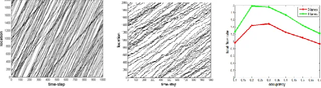
We run several simulations with cellular automaton and find that the traffic flow can be classified into two groups. The time space diagram (Figure 3) demonstrates these two kinds of traffic flow. The diagram shows the trace of every vehicle in the simulation. A gentle trace indicates a low speed. Conversely, a steep trace indicates a high speed.
Fig.3. light and heavy traffic situation: (a)Time space diagram (occupancy=0.1) (b) Time space diagram (occupancy=0.4)(c) Total flow rate under the condition of different occupancies (3 & 4 lanes)
From the left diagram, we can clearly see that the vehicles with a high speed can continue with the high speed which indicates that it is not constrained by slower vehicles. This is a situation of light traffic.
From the middle diagram, we can see that no vehicle can reach a high speed, which indicates that there is congestion. This is a situation of heavy traffic.
From the right diagram, we can see that the optimal occupancy for a 3-lane freeway and a 4-lane freeway is between 0.2 and 0.3. Thus, in our following analysis, we choose occupancy of 0.1 to represent a light traffic condition and occupancy of 0.4 to represent a heavy traffic condition.
Through study of the traffic flux, we built the model and we set the values in the model. The road’s length is 1600 cells, and the width of each cell in the road is assumed to be 7.5 m. Also, a lane’s width is 1 cell and every time-step represents 1 second. We run 20000 time-step and analyze the last 1000 steps to ensures us to obtain steady-state conditions.
The time step
t
is approximate to 1s,V
maxis equal to 5 (i.e. the maximum distancethat each vehicle move in each time step is 5 cells), which is parallel to 135km/h (5
The length of the road is define as 100 cells, which is equals to 750m. We define the
initial density for each lane as the same and the rate of change lane from right to left ( ,j j 1)
is equal to the rate ( ,j j 1)
. To conclude the conditions we gave above:
1, 2, 3... k
( , 1) ( , 1)
,
5
3
100
j j max hope
j j j j
V
V
L
(28)
Based on the models above, we present algorithms to simulate the traffic flux. And the specific simulation steps for traffic flux are as below:
(1) Initialize each cellular on speed. Then, record the vehicle velocity and position at the beginning.
(2) Set the maximum velocity
V
max,initialize each cellular on speed, record the vehicle velocity and position on start time(3) Search the first and last vehicle using the boundary conditions to control access (4) Search the first vehicle, record each vehicle to update the position and velocity by speeding up or slowing down or the stochastic slow form the first vehicle (5) Record the number of vehicles m and the average speed v, calculate the vehicle density and traffic flow
(6) If not stop, return to the step(3)
4.1. Simulation of keep-right-except-to-pass rule (Three-lane traffic flux)
When design the traffic flux under the keep-right-except-to-pass rule, we firstly consider the efficiency of our rules. Because the rules require drivers to drive at right unless overtaking, we can only consider the processes of overtaking as overtaking from right to left (1) and return to right (3).
According to the algorithm we present, we firstly analyze the three-lane traffic flux. When driving in three-lane road (Figure 4).
Fig.4. Freeway status simulation of three lane situation
Based on the process of straight driving, the 1st lane and 2nd lane will appear overtaking process, and the 2nd lane and 3rd lane will appear return-to-the-former-lane process. In figure 5(a) and figure 5(b), which are going to be the three lane and NS density-flux transition curves, the figure 5(a) shows the vehicle’s motion when at constant rate of decelerate and is lower than the critical density is free motion, and with
constant. After
is higher than the critical density, the increasing of
leads to traffic congestion. The average traffic flux is getting lower as well as the average velocityv
in the figure 5(c). Compared with NS’s curve, proper overtaking could avoid local traffic jams and increase the velocity of each vehicle, which could accelerate the traffic flux.Fig.5. Each process results under three lane situation:(a) Relationship between flux and density, (b) Relationship between velocity and density,(c) Relationship between flux and velocity.
4.2. Four-lane traffic flux
As for four-lane traffic flux (Figure 6), it is a similar process to three-lane traffic while driving.
Fig.6. Freeway status simulation of four-lane situation
The 1st lane, 2nd lane and 3rd lane have the process of overtaking from right to left. The 2nd, 3rd and 4th lane (figure 7(d)) have the process of return to the right. According to the picture below in figure 7(a), figure 7(b) and figure 7(c), the situation is also similar to the three-lane traffic.
4.3. Keep-left–except-to-pass rule
This is different from the keep-right rule. When just consider the traffic flux way, there is no difference between them. However when consider the safety, there is a big difference. Because the sit position of the driver is different between the keep-right rule and the keep-left rule [15].
4.4. Under the control of an intelligent system
When the vehicle is under the control of an intelligent system, there will be no more probability exist and the mistakes while driving could approximate as 0. So the traffic flux and the safety will get higher when under the same rules.
5.
Simulation and Result Analysis
Some inputs of our model may be hard to obtain or there might be some uncertainty in our inputs. Both these kinds of deviation might influence the result of our model. To test the robustness of our model, we implement a sensitivity analysis including percentages of vehicles, probability of randomization and probability of willing to Change Lane. We test our model in both light traffic and heavy traffic case. The analysis proves that our model does not demonstrate a chaotic behavior, showing a good sensitivity.
(F-flow rate, A-average speed, S- sharp breaking satisfaction, Q- frequency, STD- std. deviation of speed)
5.1. Percentages of Vehicles
We obtain this data from a freeway company [16]. Although the data are accurately collected, the percentages of vehicles may vary on different freeways. Therefore, we change the percentage of large vehicles (40%) by up to 15% to obtain the changes in our criteria. We observe a 16.61% increase in sharp braking frequency in the light traffic case. The other criteria changes little. In the heavy traffic case, all criteria changes little from table 2 and table 3. This indicates that our model can be used on freeways with varying percentages of vehicles.
Table 2. Sensitivity analysis—percentages of vehicles (light traffic)
status F A S F STD
-15% 0.00% -5.90% 16.60% -3.50% 6.40%
-10% 0.80% -0.40% 6.30% -0.60% 1.00%
-5% -2.60% -2.80% 13.80% -2.50% 6.60%
0% 0.00% 0.00% 0.00% 0.00% 0.00%
5% -1.20% 0.60% 0.60% -0.10% 1.00%
10% -3.80% -2.30% 0.20% -0.10% -1.70%
Table 3. Sensitivity analysis—percentages of vehicles (heavy traffic)
status F A S F STD
-15% 0.10% -6.20% -2.50% -6.30% -3.40%
-10% -1.30% -4.40% -3.20% -5.00% -0.80%
-5% 4.80% -0.80% -1.30% -1.50% 0.40%
0% 0.00% 0.00% 0.00% 0.00% 0.00%
5% 7.00% 2.60% -0.40% 2.00% 2.10%
10% 6.10% 3.60% 0.10% 4.60% 1.40%
15% 6.90% 4.40% 0.30% 5.80% 2.50%
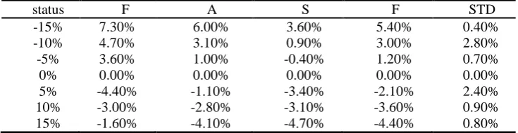
5.2. Probability of Randomization
The probability of randomization p describes the random deceleration behavior of drivers. Obviously, this parameter is difficult to obtain and it may change severely under different circumstances. In our approach, we assume it to be 0.2 since very few data on this matter are available. We change it by up to 15% and the sharp braking frequency shows a 15.75% deviation from table 4 and table 5, which is acceptable.
Table 4. Sensitivity analysis—probability of randomization (light traffic)
status F A S F STD
-15% 3.40% 0.20% -1.40% 0.40% 0.30%
-10% 0.30% 0.60% 0.40% 0.00% 1.40%
-5% 1.60% -1.80% 2.90% -0.70% 1.80%
0% 0.00% 0.00% 0.00% 0.00% 0.00%
5% 4.70% 2.30% -0.47% 0.90% -1.40%
10% 0.80% -2.00% 3.20% -0.80% 0.00%
15% -4.60% -4.90% 15.70% -3.30% 6.50%
Table 5.Sensitivity analysis—probability of randomization (heavy traffic)
status F A S F STD
-15% 7.30% 6.00% 3.60% 5.40% 0.40%
-10% 4.70% 3.10% 0.90% 3.00% 2.80%
-5% 3.60% 1.00% -0.40% 1.20% 0.70%
0% 0.00% 0.00% 0.00% 0.00% 0.00%
5% -4.40% -1.10% -3.40% -2.10% 2.40%
10% -3.00% -2.80% -3.10% -3.60% 0.90%
15% -1.60% -4.10% -4.70% -4.40% 0.80%
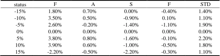
5.3. Probability of Willing to Change Lane
severe change during a short period of time. We assume probability of willing to change to the left lane and right lane are 0.5 and 0.7 respectively in our model. Therefore, we change the probabilities by up to 15% proportionally. The maximum deviation is 7.05%, which indicates a good robustness from table 6 and table 7.
Table 6.Sensitivity analysis—probability of willing to change lane (light traffic)
status F A S F STD
-15% 1.90% -0.40% 4.50% -0.80% 2.40%
-10% -3.90% -1.50% 6.70% -1.50% 4.50%
-5% 0.40% -1.60% 4.10% -0.70% 1.10%
0% 0.00% 0.00% 0.00% 0.00% 0.00%
5% 1.90% 0.50% 0.00% 0.10% 0.00%
10% -7.10% -4.70% 6.60% -3.20% 5.50%
15% -2.70% -2.40% 4.20% -1.10% 1.70%
Table 7.Sensitivity analysis—probability of willing to change lane (heavy traffic)
status F A S F STD
-15% 1.80% 0.70% 0.00% -0.40% 1.40%
-10% 3.50% 0.50% -0.90% 0.10% 1.10%
-5% 2.60% -0.20% -1.40% -1.10% 1.90%
0% 0.00% 0.00% 0.00% 0.00% 0.00%
5% 3.80% 0.80% -1.60% -0.10% 2.20%
10% 3.90% 0.60% -1.00% -0.50% 1.80%
15% -2.20% -0.50% -2.20% -0.30% 1.10%
6.
Conclusion
When the traffic flow rate is low, the keep-right rule is better in promoting the average velocity. If there are no rules, slower vehicles will not change lanes unless for overtaking. However, it brings heavy traffic. According to the existing references, a cellular automata model based on the factors include traffic flow velocity and density was used. There are the average velocity, overtaking rate road, danger index and assess the performance of the keep-right rule by comparison the unrestricted rule.
The results depend on the combination of the process of overtaking and safety. These results we get above all based on those models. In other words, hose models can handle most of the situation that similar to the traffic flux.
Rear-end collision model considers the reflection speed of drivers, the velocity and type of vehicle. It evaluates the safe distance between vehicles. What is more, lateral collision model well considers the relationship between blind angle of the driver and the safety velocity. So, the established models can determine the factors which affect security and select these factors individually after the quantitative simulation.
maximum speed limit of 108km/h (4 cell/s) and 135km/h (5 cell/s) and a case with no maximum speed limit. (The width of each cell in the road is assumed to be 7.5 m.) The maximum speed limit plays a significant role in light traffic while it is of no importance in heavy traffic are concluded. What more, the influence of minimum speed limit is studied by presenting two cases: a case with a minimum speed limit of 81km/h (3 cell/s) Vehicles will not exceed the limit due to randomization by minimum speed limit. However, they can decelerate due to safety consideration. So the minimum speed limit plays a significant role in heavy traffic while it is of no importance in light traffic.
References
1. Jamal EZ, Antoine H, Hesham R. Simulating no-passing zone violations ona vertical culve of a two-lane rural road[C]. Federal Highway Administration. In Transportation Research Board 81st Annual Meeting, No 2459. TRB, National Research Council Washington DC, 2002
2. Koorey G. Assessment of rural road simulation modeling tools[C]. IPENZ Transportation Group Technical Conference, 2002
3. Da Yang, Xiaoping Qiu, Dan Yu, Ruoxiao Sun, Yun Pu. A cellular automata model for car– truck heterogeneous traffic flow considering the car–truck following combination effect Physica A: Statistical Mechanics and its Applications, Volume 424, 15 April 2015, Pages 62-72
4. Francesco Benedetto, Alessandro Calvi, Fabrizio D’Amico, Gaetano Giunta.Applying telecommunications methodology to road safety for rear-end collision avoidance. Transportation Research Part C: Emerging Technologies, Volume 50, January 2015, Pages 150-159
5. D. Ngoduy Linear stability of a generalized multi-anticipative car following model with time delays Communications in Nonlinear Science and Numerical Simulation, Volume 22, Issues 1–3, May 2015, Pages 420-426
6. A classification of one-dimensional cellular automata using infinite computations Applied Mathematics and Computation, Volume 255, 15 March 2015, Pages 15-24 Louis D’Alotto 7. Guohua Liang, Fengjing Wang, Wei Wang, Xiaoduan Sun, Wugong Wang. Assessment of
freeway work zone safety with improved cellular automata model. Journal of Traffic and Transportation Engineering (English Edition), Volume 1, Issue 4, August 2014, Pages 261-271
8. Yo-Sub Han, Sang-Ki Ko. Analysis of a cellular automaton model for car traffic with a junction. Theoretical Computer Science, Volume 450, 7 September 2012, Pages 54-67 9. Rui Mu, Toshiyuki Yamamoto. An Analysis on Mixed Traffic Flow of Conventional
Passenger Cars and Microcars Using a Cellular Automata Model. Procedia-Social and Behavioral Sciences, Volume 43, 2012, Pages 457-465
10. Hensher, D.A.; Greene, W.H.: Specification and estimation of the nested logit model alternative normalisaions. Transp. Res.B. 36, 1–17 (2002)
11. Jinxian Weng, Shan Xue, Ying Yang, Xuedong Yan, Xiaobo Qu. In-depth analysis of drivers’ merging behavior and rear-end crash risks in work zone merging areas.Accident Analysis & Prevention, Volume 77, April 2015, Pages 51-61
12. Rami Harb, Essam Radwan, Xuedong Yan, Mohamed Abdel-Aty. Light truck vehicles (LTVs) contribution to rear-end collisions. Accident Analysis & Prevention, Volume 39, Issue 5, September 2007, Pages 1026-1036
14. http://ntl.bts.gov/
15. H. Buxton and S. Gong:“Visual Surveillance in a Dynamic and Uncertain Worl”, Artificial Intelligence, Vol. 78, pp. 431–459, 1995
Fan Zhang, Female, 07/1993, Student, Major: Finance, Zhejiang University City College, Hangzhou Zhejiang 310015, China.
Zhike Han, Male, 06/1980, Master, Research Field: Software Technology,Zhejiang University City College, Hangzhou Zhejiang 310015, China.
Hanyu Ge, Female, 10/1994, Student, Major: International Trade, Zhejiang University City College, Hangzhou Zhejiang 310015, China.
Yingping Zhu, Female, 05/1994, Student, Major: Statistic, Zhejiang University City College, Hangzhou Zhejiang 310015, China.