Principles of Analysis of Internal Structures of Aggregate Demands
Alexander MILNIKOV, Salavat SAYFULLIN
Abstract
Demand estimation problem arises each time when there is need for forecasting of the sales volume, optimal price settlement for
profit maximization, or for empirical studies of the market for demand. Because there is a relationship between price and quantity de
-manded, it is important to understand the impact of pricing on sales by estimating the demand curve for the product. The current paper introduces new method of analysis of demand internal structure and compound nature depended on the contribution of various groups of customers. Direct and inverse problem of estimation of elementary and aggregate demands parameters are defined. Aggregate demand structure is represented as a multidimensional dummy variables regression model. The theoretical results are verified by means of cor
-responding numerical example.
Keywords: market demand, aggregate demand, internal structure, price, regression analysis JEL: C13, C18, C51, C53
1. Introduction
Demand estimation problem arises each time when there is need for forecasting of the sales volume, optimal
price settlement for profit maximization, or for empirical studies of the market for demand. Because there is a rela
-tionship between price and quantity demanded, it is impor
-tant to understand the impact of pricing on sales by esti
-mating the demand curve for the product. Market demand for the product can be obtained by survey or experiments
can be performed at prices above and below the current
price in order to determine the price elasticity of demand. Alfred Marshall (1890) approached market demand curve from individual demand curves obtained by marginal utility principle, some other economists used indifference curve analysis to serve the same goal. However the appli
-cations of these two methods are difficult so econometric methods have been developed in recent years. There are researchers (for example, Kayser (2000), Mannering and Winston (1985), Archibald and Gillingham (1980)) that apply multiple regression equation to historical statistical data to form estimated market demand curve, and there are others (for example, Afriat(1967), Diewert(1973, 1985), Lansburg(1981), Varian(1982, 1983, 1985), Chavas and Cox(1997)) which use nonparametric methods to analyze behavior of consumers with observed data without specify -ing function form of the preferences or/and demand
func-tion.
Leff (1975) in his research proposed that it can be profitable to set low price and to produce at high volume level, so that business will benefit high profit and society will benefit from cheaper prices. He approached to the de
-mand curve as the horizontal summation of de-mand curves
of consumer groups separated by the amount of wealth. He suggests that the prices are set optimally in the region where most consumers can benefit from the product. If
the price is set a bit lower, then more consumers can be
reached. In other words the shape of aggregate demand curve can tell us that more profit can be obtained by setting different price(s). The total consumer group of the product can be viewed as the separate groups of consumers by their purchasing power.
In the current paper we suggest new approach to
ag-gregate demand analysis.
2. Definitions of the problems
We start with definition of basic concepts used in the article.
Observed Demand D – measured demand.
Smoothed Demand Ds – demand obtained by esti
-mating of regression equation (possibly nonlinear), on the
base of Observed Demand D
D=f (P). (eq.1)
Elementary Observed Demand Di (i=1,2,….,r) – ob
-served demands, the sum of which is equal (but not neces
-sary!) to the Observed Demand D.
Smoothed Elementary Demands Dsi(i=1,2,…,r) – which are represented by the regression equations (we assume it is linear, unlike to nonlinear equations of the
Smoothed Demand Ds), based on Observed Elementary
Demands Di.
Smoothed Elementary Demands Dsi. DAΣ is the result of
smoothing (by the vertical summation) of Observed De
-mand D.
It is assumed that the Observed Demand is
D = DAΣ + εDA. (eq.2)
We consider two different representations of Observed
Demand D: representation by regression model (1) and representation by Aggregate Demand DAΣ(2).
Above given definitions allows to formulate two mutu
-ally inverse related problems.
Direct problem. Given Smoothed Elementary De -mands Dsi, that is the set of parameters of di, it is required
to define Smoothed Demand Ds, which assumed to be equal
to aggregate values of DAΣ. It is clear that the problem can
be simply solved by calculating the value of DAΣ(zi) for the
given relative price zi. (see eq. 3)
Inverse problem. Given the Demand Di for some
val-ues of zi (i=1,….,n) and for end-prices xi (i=1,….,r) on the
interval of (0,xmax=1). It is required to define values of di
that are Smoothed Elementary Demands Dsi.
Usage of concept of aggregate demand can be justified as follows. We consider hypothetical data which clearly
shows difference between direct usage of conventional
re-gression analysis and approach based on the aggregate de
-mand model. In fig.1 the observations of three independent elementary demands are given. They can be represented by means of linear regression equations which are shown as straight dashed lines in fig.1.
Figure 1. Elementary Observed Demands and their Regression Lines.
The three clouds of elementary demand observations can be represented (by means of summation) as one cloud of demand which is shown in fig.1. Direct application of conventional regression analysis to the data of fig.2 (obser
-vation are approximated by means of second order polyno -mial) does not permit to discover the hidden fact that the
data was actually the result of interaction of three elemen
-tary demands.
Figure 2. Result of Summation of Three Elementary Demands.
This very important fact completely falls out of frame of conventional regression analysis, whereas approach based on aggregate model permits to explicit hidden in
-ternal phenomena of Demand-Price compound interaction. The above mentioned justifies importance of elabo
-ration of mathematical methods of analysis of aggregate demands.
3. Basic Part
3.1. Theoretical Basics
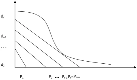
The Fig.1 represents the general case of aggregative and elementary demands structure.
Figure 1. Graphical Representation of Aggregate Demand DAΣ.
The curve is the smoothed nonlinear demand Ds,
straight lines are the smoothed elementary demands Dsi.
Pi – prices for the aggregate, where smoothed
elemen-tary demands Dsi equals to zero, i.e. they are end-prices of
smoothed elementary demands Dsi. They may be equally
spaced, or they may not be. Further we introduce unitless
(eq.3)
Pmax – where the price of nonlinear demand curve is
equal to zero.
It is obvious from this expression that 0≤х≤1 and . Besides we introduce one more variable z=x
(also unitless price), which will be used for technical
pur-poses in integration.
Let us define the aggregate demand DAΣ. The ag
-gregate demand, being the summation of elementary de -mands, can be represented as follows:
, (eq.4)
where:
i0 – value of index that is equal to the index of Pi which
satisfies ;
r – number of elementary demands
Let , then the equation (4) can be rewritten as:
(eq.5)
Or, using the unitless price it can be rewritten as:
. (eq.6)
All three equations are representations of the Aggre -gate DemandDAΣ. They are equivalent to each other, dif
-fering only in the written form, and the last one is more preferable.
Let us discuss the equation (6). Firstly, lower limit of summation is the variable value, depending on z (x and z are represent the relative price, in mathematical terms they are different: xi is the end-prices, z is the current price
from interval of (0, zmax=1)). Secondly, end-prices are fixed
known values. Thirdly, as unknowns one can consider both
DAΣ and di.
Assume that there are r intervals Δ1=(0, x1), Δi=(xi-1,
xi),…,Δr=(xr-1, xr=1) (note that xr=xmax=1) set by r values of
the end-prices, and let us suppose that values of zj (j=1,…
,n) distributed in the way that at least one of them falls into one of the intervals Δi. Let us define the quantity of zj
points, falling into ith interval, through k
i. It is obvious that
values of ki should satisfy the equality .
Thus, there are r groups of zj points randomly distrib
-uted in intervals of Δi with one condition: “at least one of
them falls into one of the intervals Δi”. Note that some of them may coincide with the end-prices. Therefore there are r unknowns of di that requires defining n≥r values of zj,
and D(zj), that results in a system of linear equations with matrix Aij:
. (eq.7)
which is rectangular for n>r and square for n=r.
It is not difficult to conclude that matrix A of system
(7) for n>r will have the following form:
(eq.8)
and for n=r:
(eq.9)
In the first case we have an overdetermined system of n × r (the number of equations exceeds the number of un
-knowns), and the ordinary least squares method should be used to determine the di, while the second case is a system of linear equations r × r.
The solution of the second case does not present dif
-ficulties and leads to the solution of the system (7) with the matrix (9), which in this case is triangular, so that the solution even can be written out analytically without em
-ploying numerical calculations.
The first case, when there is overdetermined sys
-tem (the number of equations exceeds the number of un
-knowns), requires the use of the ordinary least squares method.
It should be noted that we are modeling the depend-ence of Demand from Price, so that we are dealing with the
function of one variable D=f(P), but system (7) represents this dependence as the function of r variables: zi (i=1,…
,r). Besides in system (7) instead of zi their functions -
are used, which for j=(1,…,n) create, referring to
the language of regression analysis, matrix of obser
-vations of A of size n × r that are represented in (8). The
estimated parameters are the values of di (i = 1, ..., r) that are the intercepts of elementary demands. Thus, the prob -lem of estimating the aggregate is represented as a linear
regression problem for r variables.
3.2. Regression Model of Aggregate Demand
Consider that the data of demand price observations are given in fig.4. Assume that on the base of economical, sociological, etc. information we defined three intervals of the prices. Now we can apply the elaborated approach to try to define three elementary demands components in ini
-tial set of the data. Because there are three defined intervals of prices, r=3. The latter means that to estimate elemen
-tary demands parameters we have to use linear regression method for three dummy variables. To form a matrix of dummy variables we elaborated special program in Mat
-Lab programming language (Sayfullin, 2011).
The result of the application of the program of iden
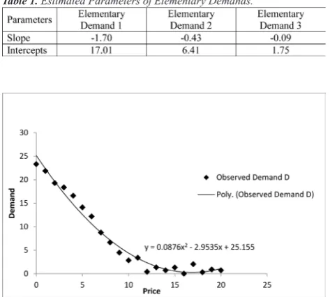
-tification of parameters of elementary demand regression lines are shown in Table 1.
One can see that observations represented in fig. 4 can be explained in terms of elementary demands which play role of components of aggregate demand. Clear that second order polynomial can also be applied to the data (fig. 5).
The later approximation can be efficiently used for
prediction and other computations connected with
de-mand-price analysis, but it does not permit, as it was men -tioned above, to unfold internal structure of the demand under consideration and to show compound nature of the
demand.
Figure 4. Observed Demand D, Elementary Demands and Aggregate
Demand DAΣ
Table 1. Estimated Parameters of Elementary Demands.
Figure 5. Second Order Polynomial Approximation of Observed De-mand D.
Aggregate analysis gives the opportunity to view the
contribution of the groups of the customers to shape of the
market demand curve, the effect of the current price on the profit of the firm, and price adjustment suggestions.
Conclusion
A new method of analysis of demand internal structure
and compound nature depended on the contribution of
var-ious groups of customers is suggested. New conceptions of Observed Demand D, Smoothed Demand Ds, Elementary Observed Demand Di, Smoothed Elementary Demands Dsi, and Aggregate Demand DAΣ are introduced. Direct and inverse problem of estimation of elementary and ag
-mand structure is represented as a multidimensional
dum-my variables regression model. The theoretical results are verified by means of corresponding numerical example.
1. Traditionally in economics literature the coordinate system is Price-to-Demand is used, whereas hereafter we shall use opposite Price-to-Demand-to-Price system.
References
Afriat, S. N. (1967). The Construction of Utility Functions from Expenditure Data. International Economic Review, 8(1), 67. Archibald, R., & Gillingham, R. (1980). An Analysis of the Short-Run Consumer Demand for Gasoline Using Household Sur
-vey Data. Review Of Economics & Statistics, 62(4), 622. Chavas, J., & Cox, T. L. (1997). On nonparametric demand anal
-ysis. European Economic Review, 41(1), 75-95.
Diewert, W. E. (1973). Afriat and Revealed Preference Theory. Review Of Economic Studies, 40(123), 419.
Diewert, W. E., & Parkan, C. C. (1985). Tests for the Consist
-ency of Consumer Data. Journal Of Econometrics, 30(1/2), 127-147.
Kayser, H. A. (2000). Gasoline Demand and Car Choice: Esti
-mating Gasoline Demand Using Household Information. Energy Economics, 22(3), 331.
Kennedy, M. (1974). An economic model of the world oil market. Bell Journal Of Economics & Management Science, 5(2), 540.
Landsburg, S. E. (1981). Taste Change in the United Kingdom, 1900-1955. Journal Of Political Economy, 89(1), 92. Leff, N. H. (1975). Multinational Corporate Pricing Strategy in
the Developing Countries. Journal Of International Busi
-ness Studies, 6(2), 55-64.
Mannering, F., & Winston, C. (1985). A Dynamic Empirical Analysis of Household Vehicle Ownership and Utilization. RAND Journal Of Economics, 16(2), 215-236.
Sayfullin, S. (2011). Horizontal Summation for Market Demand Curve, 6th Silk Road International Conference Proceedings, 186-187.
Varian, H. R. (1982). The Nonparametric Approach to Demand Analysis. Econometrica, 50(4), 945-973.
Varian, H. R. (1983). Nonparametric Tests of Consumer Behav
-ior, Review of Economic Studies, 50(1), 99-110.
Varian, H. R. (1985). Nonparametric Analysis of Optimizing Be