RESEARCH ARTICLE
RESIDUAL ANALYSIS OF PRODUCTION, EXPORTATION AND CONSUMPTION OF
ELECTRICITY IN NIGERIA
1
Alaje Daniel, T.,
*,2Fatumo Segun, A.
and
3Adeoye Tolulope
1Mathematics and Statistics Department, Osun State Polytechnic Iree, P.M.B. 301 Iree, Osun State
2Department of Computer and Information Science, Covenant University, PMB 1023, Ota, Ogun State
3Faculty of Informatics and Management, University of Hradec Kralove, Rokitanskeho 62,
Hradec Kralove CZ-50003, Czech Republic
ARTICLE INFO
ABSTRACT
This study investigates the relationship between the production, exportation and consumption of electricity in Nigeria from the period of 2000 to 2011. This shows how the knowledge of analyzing residuals can help in developing a good model for prediction. The application was restricted to a linear regression model and it was developed for predicting consumption of electricity in Nigeria. Tests based on residuals analysis such as heteroscedasticity, multicolliniarity, and autocorrdation were applied to the original consumption-model. The model passed all the tests except the test for constancy of variance, thus suggesting that the disturbance terms are heteroscedastic which was later corrected by transforming the original data using reciprocal transformation and re-tested which eventually passed the test before it was considered adequate for prediction. At the final result, it was only consumption that was linearly related.
Copyright, AJST, 2013, Academic Journals. All rights reserved
INTRODUCTION
It is an indisputable fact that electrical energy is backbone of socio-economic advancements and stability of a nation. The Power Holding Company of Nigeria (PHCN) is the body responsible for the generation, transmission, distribution, sales and administration of electricity in Nigeria. PHCN has metamorphosed through an amalgamation of the Public Work Department (PWD), the Nigerian Government Electricity Undertaking (NEU), and the National Electricity Power Authority (NEPA). NEPA took off with a generation capacity of 523.6 megawatts and rose to 5,889.4 Megawatt in 2001 till date (TOSA, O.K. KAIWJI G.S, 2000). Generation of electric power is mainly through the Electromechanical Principle - transforming mechanical energy by means of prime mover connected to the generator to electric energy. The system of electric power generation is divided into three units: Generation, Transmission and Distribution. Transmission starts from the step-up transformer to National control center and other feeder pillars in different parts of the country. The system is called the NATIONAL GRID SYSTEM. Distribution stations are connected with supplying electric power to the sub-distribution station and to the ultimate consumers. Below are the generating stations that spread all over the country:
*Corresponding author: 1
Alaje Daniel, T. and2
Fatumo Segun, A.
1
Mathematics and Statistics Department, Osun State Polytechnic Iree, P.M.B. 301 Iree, Osun State
2
Department of Computer and Information Science, Covenant University, PMB 1023, Ota, Ogun State
Table 1: Nigeria’s Generating Stations Data
S N Year Stations
Installed Capacity (MW)
Output Capacit y (MW)
1 1956 IJORA 60 15
2 1963 AFAM 696 428
3 1968 KANJI 760 450
4 1978 SAPELE 1020 330 5 1985 JEBBA 578.4 180 6 1990 EGBIN 1320 880 7 1990 SHIRORO 600 300 8 1991 UGHELLI 600 570 9 2001 AES INDEPENDENT 240 161.1 10 2001 EPS ABUJA 15 -
5889.4 -
RESEARCH METHODOLOGY
The main objection of this study therefore is to examine, by means of residual analysis whether the proposed model is appropriate for the set of data at hand. If the proposed model is not appropriate, corrective measures such as transformations of the data may have to be undertaken, or the model may need to be modified. However, to see how this can be applied to these, one serve as "the dependent variables (production) while the exportation and consumption value derived from the production serve as the independent variables. It is obvious that since it involves dependent and independent variables, simple regression will be applicable in this case as well as test
for the autocorrelation, multicollinearity and
heteroscedasticity.
ISSN: 0976-3376
Asian Journal of Science and Technology Vol. 4, Issue 07, pp.060-065, July, 2013
SCIENCE AND TECHNOLOGY
Article History: Received 14th
April, 2013 Received in revised form 14th
May, 2013 Accepted 30th
June, 2013 Published online 19th July, 2013
Data Collection
This study covers the production, exportation and consumption of electricity in Nigeria. The data used is a secondary type and was sourced from the database of central Intelligence Agency of United Stale of America via the internet. However, this study covers the production, exportation and consumption of electricity in Nigeria within the period of twelve years (2000 to 2001). The principle of least square provides a general methodology for fitting straight line models to regression data.
Linear Regression Model
This is one of the most popularly known techniques for making projection and forecasting. The main advantage of using a linear regression model is that various tests, such as
X2, t and F can be applied to the variables in the model, and
from the results of the tests, the significance of the factors and the levels of confidence attached to them could be known. In computing the parameter for the tests is the Mean Square Error (MSB), that is, the mean of sum of squared residuals must be used.
Consider the following linear regression model:
Yi = β0+ β1X1 + ei
Where Yi is the response or the dependent variable in the i
th
trail, X\ is the value of the independent variable β0 and β1 are
parameters and ei is a random error terms with mean E(ei) = 0
and variance E(ei2) = 2 for all i, j, i = j and j = 1, 2, 3, ... K.
The error terms is assumed to be independently and normally
distributed with zero mean and constant variance, that is ei ~N
(0, 2). Since residuals are similar to error terms they may be
expected to throw some light on the nature of the true error. Thus if our fitted model is correct the residuals should show tendencies that tend to confirm the following assumptions; that the error terms;
i. Are independent that is they are uncorrelated.
ii. Have zero mean
iii. Have constant variance and
iv. Follow a normal distribution.
However, several of the assumption may not be fulfilled, hence it is important to examine the aptness of the model by analyzing the residuals before further analysis based on the model is undertaken.
Residual Plots
This is a graph showing the residuals on the vertical axis and the independent variable on the horizontal axis. If the point in a residual plot is randomly dispersed around the horizontal axis then a linear regression model is appropriate for the data, else, a non-linear model is used.
Residual Variance and R-Square
The smaller the variability of the residual value around the regression line relative to the overall variability the better is the production. In most cases, the ratio would fall somewhere between these extremes, that is between 0.0 and 1.0. 1.0 minus this ratio is referred to as R-square on the coefficient of determination. The R-square value is an indicator of how well
the model fits the data. For a multiple linear regression model we make the following four assumptions.
Y1= β0+ βi X1+ β2 Xi2 + --- βk Xik + ei, i = 1, 2, --- n
1. Independence: The responses variables are independent.
2. Normality: The response variable Yi is normally
distributed.
3. Homoscedasticity: The response variable Yi all have the
same variance 2 (The term Homoscedasticity is from
Greek and mean “same variance”)
4. Linearity: The true relationship between the mean of the
response variable and the explanatory variables is straight line.
Assumptions on the Random Errors
The following four assumptions on the random errors are equivalent to the assumption on the response variables.
1. The random errors ei, are independent.
2. The random errors ei, are normally distributed.
3. The random errors ei, have constant variance 2
4. The random errors ei, have zero mean.
Residual Plots and Regression Assumption
1. The regression function is not linear
2. The error terms do not have a constant variance
3. The model fit all but one or a few outlying observations
4. The errors are not normally distributed.
5. The error terms are not independent.
The purpose is to see if there is any correlation between the error terms over time (The error terms are not independent). When the error terms are independent, we expect the residuals to fluctuate in a more or less random pattern around the base line 0.
Raw Residuals
The observe value Y; of the raw materials are given by the fitted residuals
êi = Yi – β0 – β1Xi1 – β2Xi2 ---βk Xik, i = 1, ---n
Where β0, β1……….βk, are the least square estimates of the
regression parameter.
Standardized Residuals
The standardized residuals are designed to overcome the problem of different variance of the raw residuals. The problem is solved by dividing each of raw residual by an appropriate term.
Si - ei/√1 —hii– N(0/√l —hii, (1 — hii) 2
/ 1 —hii) = N(0.
2
)
That is, the standardized residuals Si - - - , Sn are random
variables with distributions Si ~N(0, 2), Si i = 1, 2, ----n.
The observed value of the ith standardized residual is given by
Least Square Estimation of Matrix Approach to Regression
First let us consider the general multiple regressions
Y=β0+ β1Xi+ β2X2+ ... βkXk+ ei
In matrix form, suppose Y1 is the sum of ith student, and X = x1, x2 ..., xk are assumed k outside factors influencing this
mark. Therefore on the basis of n independent observation, a decision can be made on the significance of the subset of the fact
X1, X2 ... Xk.
The problem has been reduced to minimizing the error sum of square. Also, the following error terms must be noted.
ei = Y – Xβ
e1e = (Y – Xβ)1
Y – Xβ
e1e = YY1 - 2β1X1+ β1X1Xβ1
e1e = -2X1Y + 2X1Xβ = 0 at turning point
β0
And β(X1X) = X1Y
β = (X1X)-1 X1Y
Test of Significance and Confidence Intervals
To test for the significance of individual regression
co-efficient, use the t-distribution is given as t=Bl/S/a11 where
S=e2/n-15 and an a11 is the principle leading diagonal element
of the matrix.
Joint Test For β
To obtain a joint lest for F-distribution, hence, the test statistics for the test is given by F0.5 k-1 , n-k = ∑β
2 1/K-1)
(∑e2
/n-k) H0: β1= β2………. Βk = 0 is to be rejected; the
f-calculated must be greater than F-tabulated at a level of significance. Otherwise, the null hypothesis is accepted and we conclude that the overall regression plane is not significant this result provides the basis for the conventional analysis of variance ANOVA.
Heteroscedasticity
Using the ordinary least square to estimate our parameters,
assumption of constraint variance is made. That is ∑(e1e) = 0
in homoscedasticity.
Test for Heteroscedasticity
There are many method of testing for heteroscedasticity but Goldfield and Quandit test would be used for the test in this project.
Decision Rule
If R is large that is greater than F-tabulated from statistical table a level of significance reject Ho which is implies there is heteroscedasticity. Otherwise, we accept the null hypothesis, that there is homoscedasticity.
Multicollinearty
This refers to as the situation in which the variable deals one subject to two or more relations, that is where oral the independent of variables are very highly inter-correlated.
Test for Detecting Multicollinearity
The method used is based on the Frischi’s Coafluence Analysis and this shows the seriousness of the effect of multicollinearity since it depend on the degree of
intercorrelation (rx1, X1) as well as in the overall of correlation
co-efficient, that is R2Yx1,x2 ... xk, it will become co-efficient
of determination.
R2 = ∑(Y-Ŷ)2
∑(Y-Ῡ)2
Autocorrelation
One of the vital assumption in linear model is the serial
independent of the disturbances terms which implies E(ee1) =
2
in which give E (et .et + s) = 0.
Test for Autocorrelation
The Durbin-Watson test
d = ∑et – et-1)2
∑e2t
Ho: Autocorrelation does not exist Hi: Autocorrelation exist
Test for Predictive Power of the Model
After all the test mentioned earlier have been carried out, we then proceed to have a test on the estimated model to determine whether it could be used to product fork value outside the project data.
t = Y – Ŷ
C1(X1X)-1C
S E = √e1e/T-k
Where C1 is the new vector counting the value of “X” in the
period outside the used in a project S is the estimated of given by,
S2 = e1e/n-k
We use residual methods in examining the simple lineal-regression model, and the following consumption to be tested:
Linear and non linear regression function
Equation Y is said to be collected with X in a linear relationship, if change in Y would be fully explained by changed in X if other factor other than X remains unchanged.
error term = 0 in a perfect relationship. A clear departure from a linear function is a curve linear regression function. The assumption of constancy of error variance or homoscedasticity
is that the variance of e is the same for all value of the
explanatory variable depicted below:
Var (ei) = E[ei - E ei]
2
E(ei)2 = 2e constant, (If it is not satisfied in any particular
case we say that ei’s are heteroscedastic). For this study,
Goldfield Quandit test is employed.
The Assumption of Normality
The random variable ei is assumed to have a normal
distribution.as shown below:
ei ~ N(0, 2), That is ei, is normally distributed with zero
mean and constant variance.
Test for Independence
This study utilizes the Durbin Watson statistical test and it is defined as:
If this assumption is not satisfied, there is a case of autocorrelation of the random variables.
ANALYSIS AND PRESENTATION OF DATA
The original function is of the following type.
Yi = β0 + βiXi + ei
Using NCSS 2000 for analysis of y on Xi we have
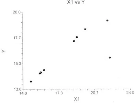
Y = 6.771338 + 0.512216 Xi
Scatter Plot Diagram to show the relationship between an independent and a dependent variable.
Figure 1: Scatter Diagram
INITIAL MODEL
Y = 4.238341+ 0.6167328X1+ 41.95213X2 SE (3.268384) / (0.1591204) (34.348) TOTAL = (1.2968) / (3.8757) (1.2214)
F = 8.0352 ttab = 2.262157
Hypothesis
1. H0:β0 = 0 Vs Hi: β0≠ 0
2. H0:β1 = 0 Vs Hi: β1≠ 0
3. H0:β2 = 0 Vs Hi: β2≠ 0
TEST INVOLVING RESIDUALS
We examine the four (4) main statistical tests based on residual analysis as mentioned above, and only two (2) are discussed in this report.
TEST FOR LINEARITY: This is a formal test for
determining whether or not the regression function is linear is F test.
Table 2: Test for linearity
S/N Year Production Xi
Consumption Yi
Predicted Value Ŷ
Residual e= y – ŷ
1. 2000 14.75 13.72 14.32652 -0.6065249 2. 2001 18.70 17.37 16.38563 0.9843667 3. 2002 15.90 14.77 14.05143 -0.1814284 4. 2003 15.67 14.55 14.79776 -0.2477036 5. 2004 15.67 14.55 14.79776 -0.2477636 6. 2005 19.85 18.43 16.93883 1.491173 7. 2006 15.59 14.46 14.75679 -0.2907864 8 2007 19.06 17.71 16.53418 1.175824 9. 2008 22.11 15.85 18.09644 -2.246435 10. 2009 22.11 15.85 18.09644 -2.246435 11 2010 21.92 19.21 17.99911 1.210886 12 2011 21.92 19.21 17.99911 1.21088
r2 (0.581506)
Table 3: ANOVA TABLE
SOURCE DF S.S MS F
Intercept 1 3190.888 3190.888
Model 1 25.30626 25.30626 13.8952s Error 10 18.21221 1.821221
Total (adjusted) 11 43.51847 3.956224
Alternative hypothesis is:
Hi: βi≠ 0
The decision rule is to control the risk of a Type 1 error and this is:
If F* ≤ F (1 – α: 1, n-2) conclude H0
If F* > F (1 – α: 1. n-2) conclude H1
F* = MSR/MSE = 25.30626 = 13.8952
1.821221
α = 0.05 since n = 10. we require F (95: 1, 10) From the table, F(95: 1,10) = 4.96
Since F* = 13.8952, and Ftab - 4.96 i.e. Fcal > Ftab which is
13.8952 > 4.16. We conclude H1, that is βi≠0 or that there is
TESTS FOR NORMALITY
The “'Goodness of fit” can be used to examine the normality
of error terms and chi-square (χ2) test can be applied for testing
the normality of error terms by analysis the residuals.
Hypothesis
H0: Error terms are normally distributed
Versus
H1 = Error terms are not normally distributed
X2 = (O – e)2/e
Where Yi is the observe value and Ŷ is the expected value
E(Y) = β0+ β1X = Ŷ
Table 4: Test for normality
Consumption Y1 (O) Predicted Value Ŷ (0 - e)2/ e
13.72 14.32652 0.02568 1737 16.38563 0.058194 14.77 14.95143 0.00220 14.55 14.79776 0.00415 14.55 14.79776 0.00415 18.43 16.93883 0.13127 14.46 14.75679 0.00597 17.71 16.53418 0.08362 15.85 18.09644 0.27887 15.85 18.09644 0.27887 19.21 17.99911 0.08146 19.21 17.99911 0.08146 1.03684
X2cal = 1.03684
Critical value: X2 = X2 (r-l)(c-l)
X21-0.05 (12-1) (2-1)
X20.95 11df = 19.68
Conclusion: Since X2cal < X2tab i.e. 1.03684 < 19.68, we
therefore accept H0 and conclude that the error terms are
normally distributed.
THE FINAL MODEL
Since the test failed as being corrected and fulfilled the new model is stated as follows:
Model
Y = 0.03401649 + 0.4982332* X (0.01256696)* (0.2i99995)*
r2 (0.339012)
*Figure in parenthesis is new standard errors.
For F – test for linearity The null hypothesis is: H0: β1 = 0
Table 5: NEW ANOVA TABLE
Source DF SS MS F
Intercept 1 4.637633E-02 4.637633E-02 Model 1 2.107527E-04 2.107527E-04 5.1289 Error 10 4.10914E-04 4.10914E-05
Total (adjusted) 11 6.216667E-04 5.651515E-05
Alternative hypothesis is:
H1: β1≠ 0
The decision rule is to control the risk of type 1 errors and this is
If F* ≤ F (1 - α: 1, n-2) conclude Ho
If F* > F (1 - α: 1, n-2) conclude H1
F* = MSR/MSE = 2.107527E – 04/4.10914E – 05 = 5.1289
α = 0.05 since n = 10, we require F (95: 1, 10)
From the table, F (95: 1, 10) =4.96
Since F* = 5.1289 and Ftab = 4.96 i.e. Fcal > Ftab which is
5.1289 > 4.16. We conclude H1 that is βi≠ 0 or that there is
linear relationship between production and consumption.
DISCUSSION OF RESULTS
From the analysis, we also have a scatter diagram showing the
linearity of Y against X1 and non-linearity against X2. Hence,
variable X2 was dropped. Because of non-linearity and the
attention was directly focus on Y against X1. That means we
can conclude that exportation X2 is not linearly related to
production i.e. exportation of electricity follows low pattern when relate to production. The regression model fitted for Y
against X1 shows that p is significance on the regression plane
and 33.9% of variation in Y are well explained by X, which implies that consumption has direct relationship with production because of the population increase and growth of companies and manufacturing industries. The new model is Z = 0.03401649 + 0.4982232M. This implies that as production increases consumption also increases as well. The real model now is Y = 29.398 + 2.007X i.e. a unit increase in production (kwt) will result in 2.007 (kwt) in consumption.
Conclusion and Recommendation
After the entire necessary test and re-test as being conducted and corrected on the data of this project. It is finally concluded that consumption of electricity plays a prominent part in the regression plane. If Nigeria will overcome the problems of abnormality, power supply, there is need to concentrate on the production. Due to the enormous consumption of electricity in Nigeria, more work should be done towards increasing the number of electricity voltage production and distribution.
REFERENCES
Adebile O.A. (2003), Statistical Method in Research (2nd
edition), Osun State.
Green O.William H. (2002): Econometrics Analysis (4th
edition) DC Health & Company, Toronto.
Kuotsytamins A. (1997): Theory of Econometrics, (2nd edition)
PP. 177/232.
Neter, T. and Wasserman, W (1974): Applied Linear Statistical Models, Richard D Irwin Inc. PP 97-136. Olayemi J.K. (1998): Element of applied Econometrics
Omotosho M.Y. (2000): Econometrics “A Practical Approach”, Ibadan. ers.
Osakwe J.O. (1982/83): Journal of Nigeria Statistical Association, Research Department Central Bank of Nigeria, Lagos.
Rapper N. and Smith H. (1996): Applied Regression Analysis (New York)
Thomas, James J. (1964): Note on the theory of Multiple Regression Analysis, Training Seminar Series 4, Athens. Tosa, O.K. Kaiwji G.S. (April, 2000)
Wooldrigla, Jefrroy M. (2000): Introduction Econometrics South Western College Publishing London
WWW. lndexmundi.com