Tutte-Equivalent Matroids

(1)

CSUSB ScholarWorks

Electronic Theses, Projects, and Dissertations Office of Graduate Studies

9-2018

Tutte-Equivalent Matroids

Maria Margarita Rocha

California State University - San Bernardino

Follow this and additional works at: https://scholarworks.lib.csusb.edu/etd

Part of the Discrete Mathematics and Combinatorics Commons, and the Set Theory Commons

Recommended Citation Recommended Citation

Rocha, Maria Margarita, "Tutte-Equivalent Matroids" (2018). Electronic Theses, Projects, and Dissertations. 759.

https://scholarworks.lib.csusb.edu/etd/759

(2)

A Thesis

Presented to the

Faculty of

California State University,

San Bernardino

In Partial Fulfillment

of the Requirements for the Degree

Master of Arts

in

Mathematics

by

(3)

A Thesis

Presented to the

Faculty of

California State University,

San Bernardino

by

September 2018

Approved by:

Dr. Jeremy Aikin, Committee Chair

Dr. Lynn Scow, Committee Member

Dr. Rolland Trapp, Committee Member

Dr. Charles Stanton, Chair, Department of Mathematics

(4)

Abstract

Matroid theory was introduced by Hassler Whitney in 1935. Whitney strived

to capture an abstract notion of independence. A matroid is composed of a finite set E,

called the ground set, together with a rule that tells us what it means for subsets of E to

be independent. We begin by introducing matroids in the context of finite collections of

vectors from a vector space over a specified field, where the notion of independence is linear

independence. Then we will introduce the concept of a matroid invariant. Specifically, we

will look at the Tutte polynomial, which is a well-defined two-variable invariant that can

be used to determine differences and similarities between a collection of given matroids.

The Tutte polynomial can tell us certain properties of a given matroid (such as the

number of bases, independent sets, etc.) without the need to manually solve for them.

Although the Tutte polynomial gives us significant information about a matroid, it does

not uniquely determine a matroid. This thesis will focus on non-isomorphic matroids

that have the same Tutte polynomial. We call such matroids Tutte-equivalent, and we

will study the characteristics needed for two matroids to be Tutte-equivalent. Finally, we

(5)

Acknowledgements

I extend my deepest gratitude to my advisor Dr. Jeremy Aikin, for his guidance

and patience in working on this project. He has been a role model as a mathematician

and teacher. I could not have done this without his help. Thank you to my committee

members, Dr. Rolland Trapp and Dr. Lynn Scow, for their support. To my mother,

Margarita Gomez-Diaz whose been so encouraging in every step. Lastly, to my fianc´e,

Bruce Valdez, who has been my pillar of support from the moment I applied to graduate

(6)

List of Figures

1.1 The geometric representation of the matroid derived from the matrixA. . 5 1.2 A rank 3 matroidM and its dualM∗. . . 8 1.3 An example of a rank 2 matroid M, and the two matroids, M −a and

M/a, after deleting an contractingafrom M. . . 10

2.1 TheW3 _{matroid. . . .} ₁₃

2.2 Computing the Tutte polynomial of a rank 3 matroid . . . 19 2.3 The matroids Q6 and R6 are the smallest examples of non-isomorphic

matroids that have the same Tutte polynomial. . . 21

3.1 The non-Fano matroidF₇− is a relaxation of the Fano matroid F7 . . . 23

3.2 Relaxing two different circuit-hyperplanes in M results in two Tutte-equivalent matroidsM_A0

1 and M

0

A2 . . . 26

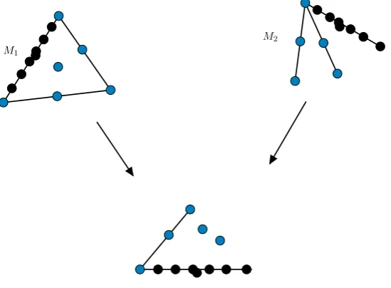
3.3 Relaxing a circuit-hyperplane from each matroid M1 and M2 results in

isomorphic relaxationsM₁0 ∼=M₂0. . . 27

4.1 Adding additional elements toM to create new Tutte-equivalent matroids. 31 4.2 Constructing additional matroids that have a common relaxation

descen-dant, by adding new elements to our ground set. . . 32 4.3 The matroid M = U2,3 ⊕U1,4 is in the only structure where a binary

matroid can have a binary relaxationM0. . . 33

(8)

Chapter 1

Introduction to Matroid Theory

Matroid theory was first introduced by Hassler Whitney in 1935, when Whitney

noticed properties of dependence common to graphs and matrices [Wel10]. Overall

matroid theory combines important ideas from linear algebra, graph theory, and finite

geometry [GM12]. Since its debut, matroid theory has grown significantly and remains

an important research area in mathematics.

1.1 Definitions

Although a matroid can be defined in many cryptomorophic ways, we will use

Whitney’s initial definition in terms of a generalized notion of independence. A matroid

M is built on a finite set of elements, E, called the ground set. Together with a family,

I, of subsets ofE calledindependent sets.

Definition 1.1.1. A matroid M consists of a finite set E, together with a family of

independent subsets I ofE, such thatI satisfies the following conditions: (I1) Non triviality: I 6=∅;

(I2) Closed under subsets: If J ∈ I and I ⊆J, then I ∈ I;

(I3) Augmentation: If I, J ∈ I with |I| < |J|, then there exists an element x ∈ J −I

such that (I∪x)∈ I.

(9)

r(X), is the cardinality of the largest independent set contained inX.

Definition 1.1.2. The rank of a matroid M is a non-negative increasing sub-modular function on subsets ofE. That is, ifA, B ⊆E, then:

(r1) 0≤r(A)≤ |A|;

(r2) If A⊆B, thenr(A)≤r(B);

(r3) r(A∪B) +r(A∩B)≤r(A) +r(B)

The rank also tells us the dimension of the geometry associated with a matroid,

according to the equation rank = dimension + 1. The maximal independent sets of a matroid are calledbases and the collection of all bases is denotedB(M). An element that is common to every basis is called a coloop, and an element that is in no basis is called a loop. Sets of a matroid that are not independent are said to bedependent. A minimal dependent set is called acircuit, and the collection of all circuits is denoted C(M).

Example 1.1.1. Consider the matroid M on the ground set E = {a, b, c, d} and with

I = {∅, a, b, c, d, ab, ac, ad, bc, bd, abd, acd, bcd}. Note that I satisfies axioms (I1), (I2),

and (I3).

• The cardinality of a maximal independent set (basis) (e.g, {abd},{acd}), is three.

Therefore, the rank of M is three.

• Notice that the element dis contained in every basis. Therefore,dis a coloop.

When a student first hears the word matroid, they might initially think of a

matrix. Indeed, a matrix over a given field is and example of a matroid. More precisely,

representable matroids are those whose ground set can be represented by the column vectors of a matrix over a field. We declare a subset of column vectors to be independent

whenever the vectors are linearly independent. A matroid that is representable over the

two element field F2 is said to be binary, and matroids that are representable over F3

are called ternary matroids. A matroid that can be represented over all fields is called a

regular matroid. One shall keep in mind, however, that not all matroids are representable. However, having a finite set of vectors as the ground set when working with representable

matroids allows us to see the independence axioms that define matroids in a more familiar

(10)

Example 1.1.2. A=    

a b c d e f

1 0 0 1 0 0

0 1 0 1 1 0

0 0 1 0 1 0



  

LetE ={a, b, c, d, e, f} be the set of column vectors of matrix A. Note that A

is a rank 3 matrix over the field F2. Now consider the column vectors having nontrivial

linear combinations that result in a zero vector. These will be the dependent sets of the

associated matroid. All other sets of column vectors will be independent.

Notice the following:

• Since f is the zero vector, f is a loop. However, any single element from E− {f}

is independent.

• There are no dependent sets of column vectors of size 2 in E − {f}. So, any

combination of two vectors fromE− {f} is independent.

• Since, (1,0,0) + (0,1,0)−(1,1,0) = (0,0,0) and (0,1,0) + (0,0,1)−(0,1,1) =

(0,0,0), we see that{a,b,d}and{b,c,e}are dependent sets. All other combinations

of three vectors taken from E− {f}will be independent.

• Any combination of four vectors is dependent.

• Thus,I ={∅, a, b, c, d, e, ab, ac, ad, ae, bc, bd, be, cd, ce, de, abc, abe, ace, acd, ade, bde,

bcd, cde}. One can check thatI satisfies the independence axioms (I1), (I2), and

(I3).

Spanning sets are subsets A ⊆E such that r(A) = r(E), and the collection of all spanning sets of a matroidM is denotedS(M). A subset F ⊆E is a flat ifF isrank maximal, meaning that for all e∈ E−F, we have r(F ∪e) > r(F). It is important to note that loops will be found in every flat (since loops have rank 0 and never increase the

rank when added to a set). A hyperplane is a flat of rankr(M)−1, and the collection of all hyperplanes of a matroid is denoted H(M).

(11)

following:

• (B1) B(M)6=∅.

• (B2) If B1, B2∈ B(M) and B1 ⊆B2, thenB1 =B2.

• (B3) If B1, B2 ∈ B(M) and x ∈B1−B2, then there exist y ∈ B2−B1 such that

(B1− {x} ∪ {y})∈ B(M).

The properties that the collection of bases, B, will be used to define a matroid

in terms of bases in future lemmas.

1.2 Geometries

There are many perspectives from which to view matroids. One of the most

advantageous perspectives is that of finite geometry, which is the perspective we will

emphasize in this thesis.

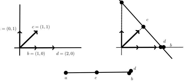
Example 1.2.1. Consider the following matrix:

A=





a b c d

1 0 1 2

0 1 1 0





Although one can easily find all the dependent and independent sets from

A, this is not an ideal approach since not all matroids can be represented by a

ma-trix. As the number of elements and rank of a matroid increases, creating a

geom-etry from the given matrix will facilitate our research. The rank of A is two, and

I(A) = {∅, a, b, c, d, ab, ac, bc, bd, cd}. Note the rank of a matroid also tells us the

di-mension of the associated geometry. So A will be a one-dimensional geometry. Next,

we will need to follow some simple guidelines to create our geometry. First, we plot the

vectors in a coordinate plane. Second, we place a line in “free” position, by making sure

it is not parallel to any of the vectors. Last, we extend or reduce the magnitude of each

vector, and/or reverse the direction of each vector so all vectors intersect the free line.

(12)

from the projected vectors (see Fig 1.1). Note, that any scalar multiple of a given vector

will result in the same projected point in the geometry.

b= (1,0)

a= (0,1) c= (1,1)

d= (2,0)

a

b c

d

a c _b

d

Figure 1.1: The geometric representation of the matroid derived from the matrix A.

1.3 Binary Matroids

A binary matroid is one that can be represented by a matrix over the field

F2. Binary matroids play an important role since they contain unimodular matroids

and graphic matroids, two fundamental classes in matroid theory [Fou87]. Additionally,

binary matroids have many attractive properties that make them an interesting class of

matroids for research.

Proposition 1.3.1. If a matroid M is binary, then each of its minors are also binary.

Matroid duality will be discussed in Section 1.4, but the following result speaks

to the importance of matroid duality in that it behaves well with respect to matroid

represent-ability over a given field.

Proposition 1.3.2. If a matroid M is binary, its dual matroid M∗ is also binary.

Example 1.3.1. A rankr matroid on a ground set withn elements is called a uniform matroid if all of its circuits are of sizer+ 1. We denote such a matroids byUr,n. Uniform

matroids play a key role in matroid represent-ability. If we are trying to determine

whether a given matroid can be represented over a certain field, we look for the existence

(13)

within” will be made more precise in Section 1.4.1, where we will explore the concept of

matroid minors. For now, an important illustration of this idea is the following theorem.

Theorem 1.3.1. A matroid is binary if and only if it does not contain the uniform matroid U2,4 as a minor.

Binary matroids can be characterized in many ways aside from not having a U2,4 minor.

Below are some useful characterizations of binary matroids. Note, ifX and Y are sets in

M, thesymmetric difference, denoted X∆Y, is equal to (X−Y)∪(Y −X).

Theorem 1.3.2. Given a matroid M, the following are equivalent: (i) M is binary.

(ii) IfC1 and C2 are distinct circuits, thenC1∆C2 contains a circuit.

(iii) IfC1 and C2 are circuits, then C1∆C2 is a disjoint union of circuits.

(iv) M has no minor isomorphic to U2,4.

(v) Every rank r−2 flat of M is contained in at most three hyperplanes.

1.4 Duality

An important tool in matroid theory is the ability to construct new matroids

from those we already know about. One of the ways to create a new matroid is through

the concept of matroid duality. The theory of duality is one of the most important tools at our disposal when attempting to solve many matroid theory problems. This theory

was first introduced by Whitney in 1935 [Oxl11]. The dual of a matroid M is another

matroid, written M∗, and it is defined on the same ground setE as follows:

Definition 1.4.1. Let M be a matroid on the ground setE. Thedual matroid M∗ will have the same ground setE such that

B(M∗) ={E−B :B ∈ B(M)}.

The rank of a subsetAinM∗is denotedr∗(A), and can be found by the following

(14)

Theorem 1.4.1. Let M be a matroid with ground set E and rank function r. IfA⊆E, then

r∗(A) =r(E−A) +|A| −r(M).

Proof. Proof of this theorem can be found in [Oxl11].

Since the rank of a matroid is determined by the cardinality of its bases, and since the

bases of the dual matroid are the complements of the bases of the original matroid, we

get the following:

Proposition 1.4.1. |E| −r(M) =r(M∗)

The compliments of spanning sets, hyperplanes, and circuits also play an

im-portant role in matroid duality.

Proposition 1.4.2. Let M be a matroid on the ground set E and suppose S ⊆E. Then

S is spanning if and only if E−S is an independent set in the dual M∗.

Proposition 1.4.3. Let M be a matroid on the ground set E. Then circuits and hyper-planes of the dual matroid M∗ are determined as follows:

(i) C(M∗) ={E−H :H∈ H(M)}

(ii) H(M∗) ={E−C:C ∈ C(M)}

Proof. (i) Let H be a hyperplane in M. If H is non-spanning, then there exists an

xi ∈ E−H such that H∪xi is spanning. Then E−H is a dependent set in M∗, and

(E−H)−xi is independent inM∗. Therefore, E−H is a circuit inM∗.

(ii) Let C ∈ C(M), so C is a minimal dependent set and is therefore not contained in any basis of M. This implies that E−C is maximal with respect to not containing a

basis complement. Thus, E −C /∈ B∗ and r∗(E−C) < r∗(B∗). Therefore E−C is a

hyperplane in M∗.

At times a matroid will contain a set that is both a circuit and a hyperplane. Let the set

of circuit-hyperplanes of a matroid M be denotedU(M).

Corollary 1.4.1.1. Let M be a matroid with the ground set E. IfU is a circuit-hyperplane of M then its compliment will also be a circuit-hyperplane in M*. That is, U(M∗) =

(15)

Example 1.4.1. Consider the matroid M with ground set E = {a, b, c, d, e} in Figure 1.2.

• By Proposition 1.4.1, r(M∗) = 2.

• The basis of M areB={abd, abe, acd, ace, bdc, bce, bde, ade}, therefore the bases of

M∗ will beB∗ ={ce, cd, bd, ae, ad, ac, bc, be}

• Since C(M) ={abc, cde, bdae}, we see thatH(M∗) ={de, ab, c}.

• By Corollary 1.4.1.1, the circuit-hyperplanes inM areU(M) ={abc, cde}, therefore

U(M∗) ={de, ab}.

M

M∗ c

a

e

c e

b

d a b

d

Figure 1.2: A rank 3 matroidM and its dualM∗.

As you may have predicted, loops and coloops also have an interesting

relation-ship in duality. We already know the bases of the dual matroidM∗ are the complements

of the bases of M. Since a coloop eis in every basis of M, we can conclude that e will

be in no basis of M∗. Therefore, we have the following:

Proposition 1.4.4. Given a matroid M, e is a loop of M if and only if eis a coloop of

M∗.

For our research. matroid duality will allow us to work with some matroids of higher

ranks that might otherwise be difficult to work with (matroids of rank 5, 6, 7...). If the

dual of the matroid in question lives in rank 0, 1, 2, 3, or 4 it sometimes is easier for the

researcher to analyze the dual of the matroid in question. We can do this because the

dual of the dual gives us to the original matroid.

(16)

1.4.1 Deletion and Contraction

Another great tool in matroid theory is the deletion and contraction opera-tions.Construction new matroids from a given matroid through a sequence of these

op-erations produces something called a matroid minor. Both operations reduce the size of the ground set E by removing a chosen element.

Definition 1.4.2. LetM be a matroid with ground setE and independent setsI. 1. Deletion: For e ∈ E, where e is not an coloop. The matroid M−e has ground

setE− {e}. The independent sets ofM−eare the sets of I that do not containe.

2. Contraction: For any element e ∈ E, where e is not a loop, the matroid M/e

has ground set E − {e} and it’s independent sets are formed by selecting all the

members of I that containe, and then removingefrom such sets.

From Definition 1.4.2, we can see why it would be inconsistent to delete an coloop e.

Recall, that coloops are in every basis of M. Our matroid M −ewould have no bases,

which implies that I = ∅, violating (I1). Now lets see why we do not contract loops.

Assume e is a loop, this implies that e /∈ I(M). We would have no independent sets to

removeefrom when creatingI(M/e). As we begin to practice these operations it would be

easier for us to start by obtaining a list of all the independent sets of the original matroid

M. We then separate the independent sets into two lists. The first those containing our

element e, and our second, those that do not contain e. When applying the contraction

operation, we will use our first list and deleteefrom any independent set. When using our

deletion operation, we will simply use our second list without any modifications. Now,

since contraction instructs us to delete e from our list of independent sets, we are also

decreasing the cardinality of our bases by one. This leads us to the following proposition.

Proposition 1.4.6. Let M be a matroid.

1. Ife is not an coloop, then r(M−e) =r(M)

2. Ife is not a loop, then r(M/e) =r(M)−1

(17)

• For M −a we adopt all the independent sets of M that do not contain a. So

I(M−a) ={∅, b, c, d, bc, cd}. Also, our new matroid M −a has remained in rank

2.

• For M/a we adopt all the independent sets of M that contain a, which are

{a, ab, ad}, and delete afrom each set. Therefore I(M/a) = {∅, b, d}. Note that c

is still in the ground set of M/a, and sincec is in no independent set, then c is a

loop. Also note, by Proposition 1.4.6, our new matroid M/ahas decreased to rank

1.

M

M/a M−a

c d

a b

c _b_d b d

c

Figure 1.3: An example of a rank 2 matroidM, and the two matroids,M−aand M/a, after deleting an contracting afromM.

Although, the conversions of our independent sets give us a lot of information

about our new minor, we also need to give some attention to what occurs to the circuits

and hyperplanes ofM.

Proposition 1.4.7. Let M be a matroid and suppose e is neither a coloop nor a loop. Then

1. Deletion: C is a circuit of M−eif and only if e /∈C and C is a circuit of M.

2. Contraction: C is a circuit of M/eif and only if

• C∪e is a circuit of M, or

• C is a circuit of M and C∪econtains no circuits except C.

Proposition 1.4.8. Let M be a matroid and suppose e is not a loop. Then H(M/e) =

(18)

The process of deletion and contraction can be completed numerous times on

the same matroid. We can delete elements of a matroid until one element remains in the

ground set. Or, we can contract elements of a matroid until we’ve arrived at a rank 0

matroid. It is also important to note that the order of operations does not matter. If we

delete aand contract b from matroid M the resulting matroid will be the same as if we

first contracted band then deleted a. This gives us the following proposition:

Proposition 1.4.9. Let M be a matroid with ground set E, and a, b ∈E. Assume the elements being contracted are not loops, and the elements being deleted are not coloops. Then,

• (M−a)−b= (M−b)−a;

• (M/a)/b= (M/b)/a;

• (M/a)−b= (M−b)/a.

When we use the operations of deletion and contraction to create new matroids,

we are producing aminor of the original matroid. Recall from Proposition 1.4.9 that the order in which we delete and contract the elements ofaandbis not important. Our only

restriction is to not delete and coloop or contract a loop.

Our next goal is to draw our new matroid minors. The deletion operation

maintains the rank of M and only deletes e from the ground set E. The geometry of

M −e will look exactly the same as M, except of course, without the element e. The

geometry for M/e will require more attention. We know that the rank of M/e will be

one less thanr(M), which means that our dimension will also decrease. The geometry of

M/eis viewed by projecting the elements ofE− {e}through the pointeonto a space of

(19)

Chapter 2

Matroid Invariants and

Tutte-Equivalent Matroids

2.1 Matroid Invariants

In mathematics a quantity is said to beinvariant if it remains unchanged under transformations. For example, geometries in a Euclidean space are invariant under

iso-metric transformations. We can find invariants in every field of mathematics, and they

are extremely useful in classifying mathematical objects. The determinant, eigenvectors,

and eigenvalues of a square matrix are invariant under a change of basis. In graph theory,

thechromatic polynomialis an invariant. Evaluating the chromatic polynomial yields the number of k-colorings of any graphG, and this is invariant under graph isomorphism.

Matroid theory has several invariants. The most notable are thecorank-nullity polynomial

and Tutte polynomial. The latter will be the focus of our research. The Tutte polynomial captures a considerable amount of information about the matroid in question. However,

not all invariants, including the Tutte polynomial are complete invariants.

Definition 2.1.1. A matroid isomorphism invariant is a function f on the class of all matroids such that f(M) =f(N), whenM ∼=N.

The theory of invariants in matroid theory originated in graph theory, in the

(20)

2.2 Corank-Nullity Polynomial

In 1932, Whitney introduced a polynomial that can be computed for any matroid

with rank function r [Wel10]. The polynomial is a two variable polynomial, having

independent variables x and y.

Definition 2.2.1. The corank-nullity polynomial of a matroid M with a ground set E

and rank r is defined as:

s(M;x, y) = X

A⊆E

xr(E)−r(A)y|A|−r(A),

where the corank of A⊆E isr(E)−r(A) and nullity is |A| −r(A).

Notice that the corank-nullity polynomial is a matroid invariant. If we are given

two isomorphic matroids M and N containing the same ground set, then every subset

A ⊆ E(M) will have a corresponding subset in N, A0 ⊆ E(N). Thus every term of

the corank-nullity polynomial ofs(M;x, y) will have a corresponding term in the

corank-nullity polynomial of s(N;x, y).

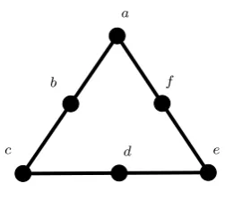
a

c e

b f

d

(21)

Example 2.2.1. Refer to the matroid W3 _{in Figure 2.1. The table below describes the}

computation ofs(W3_;_{x, y}_{) by looking at all subsets}_A _of_E₍_W3₎ _jnjnjnj

Polynomial of W3

A r(A) |A| r(E)−r(A) |A| −r(A) xr(E)−r(A)y|A|−r(A)

∅ 0 0 3 0 x3

a 1 1 2 0 x2

ab 2 2 1 0 x

abc 2 3 1 1 xy

abd 3 3 0 0 1

abcd 3 4 0 1 y1

abcde 3 5 0 2 y2

E 3 6 0 3 y3

Adding up the terms in the last column along with counting the possible ways

of obtaining our sets gives us:

s(M;x, y) =x3+ 6x2+ 15x+ 3xy+ 17 + 15y+ 6y2+y3

2.3 The Tutte Polynomial

Tutte’s motivation for his polynomial was inspired by the chromatic polyno-mial,χ(G, λ). Initially called thedichromatic polynomial, Henry Crapo later generalized Tutte’s work to matroids, and Brylawski proved many further results concerning the

Tutte polynomial [GM12].

Definition 2.3.1. Given a matroidM on ground setE, theTutte polynomial,t(M;x, y), can be computed recursively as follows:

For any element eof M, ife is neither a loop nor an coloop, then

t(M;x, y) =t(M−e;x, y) +t(M/e;x, y). (2.1)

If eis a loop, then

t(M;x, y) =y·t(M−e;x, y). (2.2)

If eis an coloop, then

t(M;x, y) =x·t(M/e;x, y). (2.3)

If E=∅, we define

(22)

The Tutte polynomial is a special evaluation of the corank-nullity polynomial.

Notice that r(M) is the highest power of x in t(M;x, y) while the nullity, n(M), is

the highest power of y in t(M;x, y). Therefore rank and nullity are invariants that are

computed by the Tutte polynomial. Additionally, since|E|=r(M)+n(M) the cardinality

of the ground set is also a Tutte polynomial invariant [BO92].

Theorem 2.3.1. The Tutte polynomial for a given matroid M is an evaluation of the corank-nullity polynomial, and a well defined matroid invariant.

t(M;x, y) =s(M;x−1, y−1)

Proof. Assume|E|= 1. Theneis either a loop or a coloop. If eis a loop thenr(E) = 0, and we get

s(M;x, y) =xr(E)−r(E)y|E|−r(E)+xr(E)−r(∅)y|∅|−r(∅)

=x0−0y1−0+x0−0y0−0

=y+ 1.

Therefore t(M;x, y) =y, and it follows thatt(M;x, y) =s(M;x−1, y−1).

If eis a coloop, thenr(E) = 1, so

s(M;x, y) =x1−1y1−1+x1−0y0−0

=x+ 1.

Therefore t(M;x, y) =x, and it follows thats(M;x−1, y−1) =t(M;x, y).

Now let |E| ≥ 2, and assume our theorem holds for all matroids on n−1 elements. We

need to show it holds for matroids on n elements. Let e ∈ E. Case 1: Assume e is neither a loop nor a coloop.We will denote r for the rank ofM,r0 for the rank function

of M−e, and r00 for the rank function of M/e. Thus,r0(A) =r(A) for allA⊆E− {e},

and r00(A−e) =r(A)−1, when e∈A.

The ground setEwill be separated into two classes. The classS1 will be the collection of

(23)

s(M;u, v) = X

A∈S1

ur(E)−r(A)v|A|−r(A)+ X

A∈S2

ur(E)−r(A)v|A|−r(A).

(1) SupposeA∈S, wheree∈A. Since the rank is lowered by one inM/e, then for each

of the subsets r00(A−e) =r(A)−1. Also, the corank of A equals the corank of A−e

computed in M/e. Thus, we have the following equation:

r(E)−r(A) =r00(E−e)−r00(A−e).

For the nullity, the rank and cardinality will both decrease by one when we remove e.

This implies

|A| −r(A) =|A−e| −r00(A−e).

Therefore,

X

A∈S1

ur(E)−r(A)v|A|−r(A)= X

A∈S1

ur00(E−e)−r00(A−e)v|A−e|−r00(A−e)

= X

B⊆E−e

ur00(E−e)−r00(B)v|B|−r00(B)

=s(M/e;u, v)

(2) Now supposeA∈S2. Sincee /∈A, thenr(E) =r0(E−e) andr(A) =r0(A). Therefore,

X

A∈S2

ur0(E−e)−r0(A)v|A|−r0(A)

=s(M −e;u, v).

Upon combining these equations, we obtain

s(M;u, v) =s(M/e;u, v) +s(M−e;u, v).

But, by definition, t(M;x, y) = t(M/e;x, y) +t(M −e;x, y). Applying our induction

hypothesis to this equation we have:

t(M;x, y) =s(M/e;x−1, y−1) +s(M −e;x−1, y−1)

=s(M;x−1, y−1).

(24)

(1) Consider the setsAinS1. The corank and nullity ofAcomputed inM are the corank

and nullity of A−e computed inM/e. Therefore, we have

X

A∈S1

ur(E)−r(A)v|A|−r(A) =s(M/e;u, v).

Now, if Ais a set in S2, because eis a coloop, we will comparer(A) and r00(A) inM/e.

When e /∈ A, we have r(A) = r00(A) in M/e, since contracting the coloop does not

affect the rank of the sets not containing e. So our corank will change in M/e, where

r(E)−r(A) = (r00(E) + 1)−r00(A), but our nullity will remain unchanged,|A| −r(A) =

|A| −r00(A). Then,

X

A∈S2

A⊆E−{e}

u(r00(E−e)+1)−r00(A)v|A|−r00(A)

=u· X

A⊆E−{e}

ur00(E−e)−r00(A)v|A|−r00(A)

=u·s(M/e;u, v).

Adding the results from the sets in S1, and the sets in S2, we get

s(M;u, v) =s(M/e;u, v) +u·s(M/e;u, v)

= (1 +u)·s(M/e;u, v)

Butu=x−1 andv=y−1, so

s(M;u, v) = (1 + (x−1))s(M/e;x−1, y−1)

=x·t(M/e;x, y).

Case 3: Assume e is a loop. We again partition our subsets in the same manner as in previous cases. For S1, since e is a loop and e∈ A, then r(A) = r0(A) in M −e. Our

corank will remain the same in M−e, r(E)−r(A) =r0(E−e)−r0(A), and our nullity

will change, |A| −r(A) =|A| −(r0(A)−1). Then,

X

A∈S1

A⊆E−{e}

ur0(E−e)−r0(A)v|A|−(r0(A)−1)

=v· X

A⊆E−{e}

(25)

For S2, sincee /∈A, we have r(E)−r0(E−e) and r(A) =r0(A). Therefore,

X

A∈S2

A⊆E−{e}

=s(M −e;u, v)

Adding the results from the sets in S1, and the sets in S2, we get,

s(M;u, v) =v·(M−e;u, v) +s(M/e;u, v)

= (v+ 1)·s(M −e;u, v).

But u=x−1 and v=y−1, so

s(M;u, v) = (y−1 + 1)s(M−e;x−1, y−1)

=y·t(M−e;x, y).

Although the Tutte polynomial is simply a special evaluation of the

corank-nullity polynomial, the Tutte polynomial allows us to recursively compute the polynomial

of a geometry or graph by using deletion and contraction. Ultimately, we will arrive at

a collection of matroid minors whose Tutte polynomials we know. The sum of these

polynomials gives us the Tutte polynomial for the given matroid.

Example 2.3.1. Consider the matroid Q6 in Figure 2.2. The last row of the figure contains matroids U2,3,U1,3,U2,2,U1,1⊕U0,1, andU0,3. The Tutte polynomials of these

matroids are:

• t(U2,3;x, y) =x2+x+y

• t(U1,3;x, y) =x+y+y2

• t(U2,2;x, y) =x2

• t(U1,1;x, y)·t(U0,1;x, y) =xy

• t(U0,3;x, y) =y3

(26)

e

−e _/e

−e /e

x( )

−e /e

−e

x+1( ) +3( )+( )+( )+( )

/e

−e

−e /e

−e e

e

Q6

Figure 2.2: Computing the Tutte polynomial of a rank 3 matroid

One can find the rank and cardinality of the ground set visually. In Example

2.3.1 the rank of Q6 is three and the ground set contains six elements. However, this is

only a small amount of information that the Tutte polynomial tells us.

Proposition 2.3.1. For any matroid M, the Tutte polynomial captures the following information:

• t(M; 1,1)gives the number of bases of M.

• t(M; 2,1)gives the number of independent sets of M.

• t(M; 1,2)gives the number of spanning sets of M.

• t(M; 2,2) = 2|E|, the number of subsets of M.

(27)

Tutte polynomial. Basically, if we know the Tutte polynomial of any given matroid, we

also know the Tutte polynomial of its dual.

Theorem 2.3.2. Given a matroid M, the Tutte polynomial of the dual matroid M∗ is found by

t(M∗;x, y) =t(M;y, x). (2.5)

Proof. We will use the corank-nullity polynomial for this proof. Additionally, recall that that the Tutte polynomial is an evaluation of the corank-nullity polynomial. Therefore,

s(M;u, v) = X

A⊆E

(x−1)r(E)−r(A)(y−1)|A|−r(A).

Before we begin, recall the following relationships:

Using Theorem1.4.1, the rank of the set A in the dual matroid is given by

r∗(A) =r(E−A) +|A| −r(E).

The corank is

r∗(E)−r∗(A) =|E| −r(E)−[r(E−A) +|A| −r(E)]

=|E−A| −r(E−A).

Also, the nullity is

|A| −r∗(A) =|A| −[r(E−A) +|A| −r(E)]

=r(E)−r(E−A).

Notice the corank of A inM∗ is equal to the nullity ofE−AinM, and the nullity ofA

(28)

From the observations, it follows that

s(M∗;u, v) = X

A⊆E

(x−1)r∗(E)−r∗(A)(y−1)|A|−r∗(A)

= X

A⊆E

(x−1)|E−A|−r(E−A)(y−1)r(E)−r(E−A)

= X

A⊆E

(x−1)r∗(E)−r∗(A)(y−1)|A|−r∗(A)

= X

A⊆E

(x−1)|A0|−r(A0)(y−1)r(E)−r(A0)(∵A0 =E−A)

=s(M;y−1, x−1).

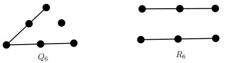
Our question now is to what extent does this information determine a unique

matroid. In other words, given two matroids that have the same Tutte polynomial, is it

possible that they will always be isomorphic? The answer is no. If we observe the two

matroids in Figure 2.3 we can see that although both matroids having the same Tutte

polynomial, the matroids are non-isomorphic. The remainder of this thesis is dedicated

to studying such matroids.

Q6 R6

Figure 2.3: The matroidsQ6andR6are the smallest examples of non-isomorphic matroids

(29)

Chapter 3

Matroid Relaxation

3.1 Matroid Relaxation and the Tutte Polynomail

A matroid operation that has allowed one to find other matroids is calledmatroid relaxation. Several well known matroids have been created through this operation, the Fano and non-Fano matroids, Pappus and non-Pappus matroids are just two examples

of this operation. Both, matroids have the same ground sets and almost the same bases.

This operation in particular will be very fruitful in finding Tutte-equivalent matroids.

Definition 3.1.1. If M1 and M2 are two non-isomorphic matroids that have the same

Tutte polynomial such that t(M1;x, y) = t(M2;x, y), then we say that M1 and M2 are

Tutte-equivalent.

Definition 3.1.2. Let M be a matroid having a subset A ⊂ E such that, A is both a circuit and a hyperplane. Relaxing A will result in a new matroid M0 with a new set of bases on the same ground set E such that B0 = B(M)∪A. Additionally, C(M0) =

C(M)−A.

When a circuit hyperplane A is relaxed in matroid M, our new matroid will be denoted

M_A0 . The pressing issue now, is to prove that relaxing a circuit hyperplane does result in a new matroid.

(30)

F7 _F− 7 relax{4,5,6}

1

2 3

7

4 6

5

1

2 3

7

4 6

5

Figure 3.1: The non-Fano matroid F₇− is a relaxation of the Fano matroid F7

Proof. Assume M contains a circuit-hyperplane A ∈ C(M) and a collection of basis

B1, B2, B3, . . . Bn ∈ B(M). By definition, relaxing A will result in a new matroid M_A0

where B(M0) =A∪ B(M). ThereforeM0 will satisfy ourB3 axiom in two cases.

Case 1: For allx∈A, there exist y∈Bi (for any i) such thatA− {x} ∪ {y} ∈ B(M0).

Let A ∈ C(M), so A− {x} ∈ I(M), now assume with out loss of generality, there exist

B2 ∈ I(M). So in M we have two independent sets I1 = A− {x} and I2 = B2, where

|I1|<|I2|. Then by our independent axiomI3, there exist an elementy ∈ I2−I1 such

that I1∪ {y} ∈ I(M). Additionally I1∪ {y} ∈ B(M).

But I1∪ {y}= (A− {x})∪ {y}. Since (A− {x})∪ {y} ∈ B(M) and B(M0) =B(M)∪A,

then we know (A− {x})∪ {y} ∈ B(M0).

Case 2: For allx∈Bi (for anyi), there existy∈A such thatBi− {x} ∪ {y} ∈ B(M0).

Assume A∈ B(M0) andB2∈ B(M). We need to show that there exist an elementy∈A

such thatB2−{x}∪{y} ∈ B(M0). If no suchyexist, then (B2−{x})∪{y}=r(M)−1 for

ally ∈A. Then we can assume thatyis in the closure ofB2− {x}andr(B2− {x})∪A=

r(M)−1. A contradiction.

Being able to create an additional matroid M0 from the original M is a

pow-erful tool when we are trying to find matroids having the same rank and ground set.

Additionally, if a matroid contains n circuit hyperplanes we can relax said matroid to

create at most n new matroids. The next question in order is, once we have relaxed a

circuit hyperplane and created a new matroidM0how does it affect the Tutte polynomial.

Luckily, one does not need to find the Tutte polynomial from scratch.

(31)

can be computed as follows,

t(M0;x, y) =t(M;x, y)−xy+x+y (3.1)

Proof. We will prove this theorem using the corank-nullity polynomial. Let M be a matroid with Bn ∈ B(M), and circuit-hyperplanes A1, A2, A3...An ∈ A(M). The set of

circuit-hyperplanes are computed in the corank-nullity polynomial as follows:

Recall the rank and cardinality of A are, r(A) =r(E)−1 and|A|=r(E),

X

A⊆E

ur(E)−(r(E)−1)vr(E)−(r(E)−1)

X

A⊆E

u1v1

.

The sets of bases, B(M), will also be computed at follows:

X

B⊆E

ur(E)−r(E)vr(E)−r(E)

X

B⊆E

u0v0

The circuit-hyperplanes and basis sections for our corank-nullity polynomial will be

de-scribed as

s(M;u, v) =. . .+i(uv) +j(1) +. . .

where irepresents the number of circuit hyperplanes and j the number of basis found in

M.

Without loss of generality we’ll now relax the circuit hyperplane A1 of M. Doing so,

we will obtain a new matroid M0 on the same ground set E whose basis will become

B(M0) =B(M)∪A1 andC(M0) =C(M)−A1.

(32)

s(M;u, v) =. . .+ (i−1)(uv) + (j+ 1)(1) +. . .

Recall that the Tutte polynomial is an evaluation of the corank-nullity polynomial,

t(M;x, y) = s(M;x−1, y −1). Then, we can redefine the corank-nullity polynomial

of M as:

t(M;x, y) =. . .+i(x−1)(y−1) +j(1) +. . .

t(M;x, y) =. . .+ixy−ix−iy+ (i+j) +. . .

Matroid M0 will be defined as

t(M0;x, y) =. . .+ (i−1)(x−1)(y−1) + (j+ 1)(1) +. . .

t(M0;x, y) =. . .+ixy−ix−iy+ (i+j)−xy+x+y+. . .

We can see that the difference between the Tutte polynomial ofM andM0 is−xy+x+y.

Therefore, when a circuit hyperplane of a matroidM is relaxed, we obtain a new matroid

M0 whose Tutte polynomial can be derived by

t(M0;x, y) =t(M;x, y)−xy+x+y

3.2 Parent and Descendant Matroids

The matroid relaxation tool has given us the ability to find at least one other

matroid with the same ground set and rank as our original. However, if a matroid contains

at least two or more circuit-hyperplanes it can produce two non-isomorphic matroids as

well.

Definition 3.2.1. Assume we have two non-isomorphic matroidsM1 andM2where each one contains at least one circuit hyperplane. If we relax each matroids respective

circuit-hyperplane so that M₁0 andM₂0 are isomorphic, then we can define M1 andM2 as having

a common relaxation descendant. See Figure 3.3

Definition 3.2.2. Assume we have a matroid M containing at least two circuit-hyperplanes, A1 and A2. If we can relax each circuit-hyperplane individually such that

(33)

M

M_A0₁ M_A0₂

A1 ={3,4,5} A2 ={5,6,7} 1 3 ₅ 7 2 4 6 3 1 5 7 4 2 6 1 3 5 2 4 6 7

Figure 3.2: Relaxing two different circuit-hyperplanes inMresults in two Tutte-equivalent matroids M_A0

1 andM

0

A2

.

Approaching matroids by finding a common relaxation descendant or common relaxation

parent allows us to find non-isomorphic matroids that will aways have the same Tutte

polynomial.

Corollary 3.2.0.1. If two matroids,M1 andM2 have a common relaxation descendant,

such that M₁0 ∼=M₂0 thent(M1;x, y) =t(M2;x, y).

Proof. Assume we have two matroidsM1 and M2 and we relax each matroid to discover

that M₁0 and M₂0 have isomorphic relaxations. By Theorem 3.1.2, we know the Tutte

polynomial of M₁0 andM₂0 will be t(M₁0;x, y) =t(M1;x, y)−xy+x+yand t(M20;x, y) =

t(M2;x, y)−xy+x+y respectively. Since the relaxations of M1 andM2 are isomorphic

their polynomials will be equal. That ist(M1;x, y)−xy+x+y=t(M2;x, y)−xy+x+y

If we wish to obtain the Tutte polynomial of the original matroid, we have to perform some

algebraic manipulation to the polynomial of the relaxed matroid. Thereforet(M1;x, y) =

t(M2;x, y).

The Tutte polynomial of matroid that is a common relaxation parent can be found as

(34)

Corollary 3.2.0.2. Suppose a matroid M contains at least two circuit-hyperplanes

A1, andA2, such that the respective relaxations result in two non-isomorphic matroids,

M_A0

1 M

0

A2. Then, Tutte-polynomials t(M

0

A1;x, y) =t(M

0

A2;x, y).

Proof. This proof follows from Theorem 3.1.2.

M1 _M2

M0 = (M₁0 ∼=M₂0)

(35)

Chapter 4

Classifying Tutte-Equivalent

Matroids

We have seen that the Tutte polynomial encodes a significant amount of

infor-mation about a matroid. Additionally, we have found a method to find Tutte-equivalent

matroids through matroid relaxation. The task now is to classify Tutte-equivalent

ma-troids. In what follows, we will develop additional tools to construct Tutte-equivalent

matroids within certain matroid classes. We begin by determining restrictions on the

rank and the cardinality of the ground set for Tutte-equivalent matroids.

Lemma 4.1. Any two rank 0 Tutte-equivalent matroids are isomorphic.

Proof. AssumeM1andM2 are two matroids in rank 0 each on the samen-element ground set. All elements in a rank 0 matriod are loops, hence there is only one way to build such

a matroid. Therefore, all such matroids will be isomorphic.

Additionally, we can easily compute the Tutte polynomial for rank 0 matroids on n

elements:

t(U0,n;x, y) =yn (4.1)

Lemma 4.2. Any two rank 1 Tutte-equivalent matroids are isomorphic.

Proof. Suppose we have two matroids M1 and M2, such that t(M1;x, y) = t(M2;x, y).

Necessarily, both matroids must contain the same number of loops and parallel elements

(36)

elements, respectively, in matroid Mi. However, since parallel elements in rank 1 can

only occur in a single parallel class, then the two matroids must be isomorphic.

For a rank 1 matroid M on n elements, containing ` ≥0 loops and n−` ≥1

parallel elements, it is not difficult to compute the Tutte polynomial of M:

t(M;x, y) =y`(x+y+y2+....+yn−`) (4.2)

Computing the Tutte polynomials for rank 2 matroids becomes more

compli-cated, since such matroids can contain multiple parallel classes of elements. We first

compute the Tutte polynomial for U2,n, where n ≥ 2. This can be seen by noticing

that any single element contraction in U2,n produces the matroidU1,n−1, while any single

element deletion in U2,n produces the matroid U2,n−1 (ifn≥3).

t(U2,n;x, y) =

x2+ (n−2)x+ (n−2)y+ (n−3)y2+...+ (n−k−1)yk+...yn−2 (4.3)

The Tutte polynomials for rank 2 matroids that contain ` ≥ 1 loops, but no parallel

elements have the following formula:

t(M2,n;x, y) =

y`(x2+ (n−`−2)x+ (n−`−2)y+ (n−`−3)y2+...

+ (n−`−k−1)yk+...+yn−`−2) (4.4)

If a rank 2 matroid contains ` ≥ 0 loops and k parallel classes of size m1, m2, ...mk,

where mi ≥2, then the Tutte polynomial forM is:

t(M2,n;x, y) =

yl

h Pk

j=1

Pmj−1

i=1 x+y+y2+...yn −Pj

r=1mr+(j−2)

+ x2+ (N−2)x+ (N−2)y+ (N −3)y2+...+yN−2

i

, (4.5)

where N =n−Pk

r=1mr+k.

(37)

Proof. Assume we have two matroids M1 and M2 in rank 2 that have the same Tutte polynomial. Then, both matroids will have the same number of loops, single elements

and the same number of parallel elements in each parallel class. Each parallel class of

elements, will correspond to a unique place on an affine line. Reordering these parallel

classes on this line simply creates isomorphic copies of M1 and M2, thus resulting in

isomorphic matroids.

The implications of these lemmas is that our search of Tutte-equivalent matroids

must begin in rank 3 and higher. However, as we see in the next results, the ground sets

of two Tutte-equivalent matroids must also not be too small with respect to the ranks of

the matroids. To prove this we recall Theorem 2.3.2, which implies the following:

Corollary 4.0.0.1. If M1 and M2 are Tutte equivalent matroids, t(M1;x, y) = t(M2;x, y), then t(M1∗;x, y) =t(M2∗;x, y)

Proof. SinceM1andM2are Tutte-equivalent, thent(M1;x, y) =t(M2;x, y). By Theorem 2.3.2 t(M₁∗;x, y) = t(M1;y, x) and t(M₂∗;x, y) = t(M2;y, x). Therefore t(M₁∗;x, y) =

t(M₂∗;x, y).

Corollary 4.0.0.2. IfM1 andM2 are Tutte-equivalent matroids, each having rankr ≥3, then |E(Mi)| ≥r+ 3, for i= 1,2.

Proof. Suppose, to the contrary, thatr≤ |E(Mi)|< r+ 3, for some i. SinceM1 andM2

are Tutte-equivalent, |E(M1)|=|E(M2)|. Therefore, r≤ |E(M1)|=|E(M2)|< r+ 3. If

|E(M1)|=|E(M2)|=r, thenr(M₁∗) =r(M₂∗) = 0, and by Lemma 4.1, M₁∗ ∼=M₂∗, which

impliesM1 ∼=M2. This contradicts the hypothesis thatM1 andM2 are Tutte-equivalent.

If |E(M1)|=|E(M2)|=r+ 1, then r(M1∗) =r(M2∗) = 1, and by Lemma 4.2,M1∗ ∼=M2∗,

which implies M1 ∼= M2. This again contradicts the hypothesis that M1 and M2 are

Tutte-equivalent. Finally, if |E(M1)|=|E(M2)|=r+ 2, then r(M1∗) =r(M2∗) = 2, and

by Lemma 4.3, M₁∗ ∼= M₂∗, which implies M1 ∼= M2. This once again contradicts the

hypothesis that M1 and M2 are Tutte-equivalent. Therefore, it follows that |E(Mi)| ≥

r+ 3, fori= 1,2.

Thus, our search for Tutte-equivalent matroids must begin with rank 3

ma-troids having at least six elements. Figure 2.3 illustrates the smallest example of

(38)

A1

A2

Figure 4.1: Adding additional elements toM to create new Tutte-equivalent matroids.

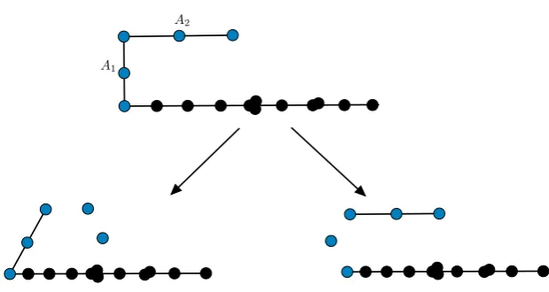
Once we have found a matroid M that is a common relaxation parent to at least two

matroidsM₁0 andM₂0 we can continue to relax circuit hyperplanes inM₁0 andM₂0 in hopes

of finding additional Tutte-equivalent matroids, See Figure 5.1. Additionally, we can also

use our parent matroid M as the foundation to construct new matroids by adding new

elements to our ground set. The only restrictions are:

1. An element eadded to the ground set cannot be a loop.

2. Elements cannot be added to the circuit-hyperplanes A1 and A2.

Example 4.0.1. The matroid in Figure 3.2 is in rank 3 with|E|= 7. We can construct another matroid in the same rank that is also a common relaxation parent by adding 10

additional elements as in Figure 4.1.

A similar approach is applied to matroids M1 and M2 that share a common relaxation

descendant with one additional restriction. See Figure 4.2.

1. Any element eadded to the ground set cannot be a loop.

2. Elements cannot be added to circuit hyperplane A.

3. The same amount of elements or parallel classes must be added to both M1 and

M2.

Our initial research began by finding ways to construct and classify Tutte-equivalent

(39)

quickly became a very useful tool to find Tutte-equivalent matroids. Matroid relaxation

along with the correct rank and ground set gave way to a plethora of Tutte-equivalent

matroids. However, our success in constructing Tutte-equivalent matroids has made it

very difficult to classify them in any order. Therefore, we will turn our attention to

explore the existence of Tutte-equivalent matroids in classes of matroids, particularly

the binary field. We will try to find additional restrictions, if any, that Tutte-equivalent

matroids need to hold to be in the binary field. Additionally, attempting to determine if

common relaxation parents, or common relaxation descendants, will also produce binary

matroids and other questions.

M1

M2

Figure 4.2: Constructing additional matroids that have a common relaxation descendant, by adding new elements to our ground set.

4.1 Binary Descendant and Parent Matroids

Binary matroids follow the same restrictions we have established for all

matroids. To find Tutte-equivalent binary matroids they must must be in rank 3 or

higher and contain r+ 3 elements. However, binary matroids can only contain at most

2r−1 elements. So for example, a matroidM withr(M) = 4 can have a ground set that only contains from 7≤ |E| ≤15 elements.

(40)

relax={a, b, c}

M M0

a c b g f e d a c g f e d b

Figure 4.3: The matroid M =U2,3⊕U1,4 is in the only structure where a binary matroid

can have a binary relaxation M0.

results we’ve found from this class.

Definition 4.1.1. Let M1 and M2 be two matroids on disjoint ground sets E1 and E2

respectively. The direct sum is a new matroid M1⊕M2 with ground set E = E1∪E2

and independent sets I1∪I2.

Lemma 4.4. A binary matroid in rank r with ground set |E| = n that has a binary relaxation can only be in the structure of Ur−1,r⊕U1,n−r.

Proof. Given a matroidM, its circuit-hyperplane is in the structure ofUr−1,r containing r

r−2

flats. Any r−2 flat will be contained in two hyperplanes. The first,r−2∈A and

the second is composed of Hi = (r−2)∪U1,n−r.Upon relaxing the circuit-hyperplane A

we turned our dependent set independent, and increased the number of hyperplanes by

one as well. Thus evey r−2 flat will be contained in at most three hyperplanes, and will

continue to satisfy Theorem 1.3.2.

IfM is a binary matroid with two Tutte-equivalent relaxationsM₁0 andM₂0, thenM must

contain at least two circuit hyperplanes and a ground set of at leastr+ 3 elements, where

every r−2 flat is contained in at most 3 hyperplanes.

(41)

Proof. IfM is a binary matroid where everyr−2 flat is contained in at most 2 hyper-planes, then M = Ur−1,r⊕U1,n−r. Thus, M is not a common relaxation parent. Now

assume M is a binary matroid, and every r−2 flat is contained in three hyperplanes.

If we relax A1, then there will exist a r −2 flat in A1 contained in more than three

hyperplanes. The same result will follow for A2. Therefore, M10 and M20 are not binary

matroids.

Lemma 4.6. Common relaxation descendant binary matroids do not exist.

Proof. Suppose, to the contrary. Assume M1 and M2 are two non-isomorphic binary matroid containing circuit-hyperplanes A1 and A2 respectively. Assume relaxing each

matroids’ circuit-hyperplane gives a binary relaxation where, M_A0

1

∼

=M_A0

2. From Lemma

4.4, the only binary matroids with a binary relaxation have structure of Ur−1,r⊕U1,n−r.

Therefore, if M_A0

1 and M

0

A2 are binary, thenM1

∼

=M2.

Although it is possible to find a binary matroid that is a common relaxation parent to

two new matroids, once we relax a circuit hyperplane we’ve left our binary class. For

example the Fano matroid F7 can produce thirteen new matroids, none of which will be

(42)

Chapter 5

Conclusion

The goal of this thesis was to identify and study matroids that have the property

of being Tutte-equivalent. We began learning that every matroid can be represented by

a Tutte polynomial, and said polynomial encodes several pieces of information about our

matroid. Such as:

• t(M; 1,1) gives the number of basis ofM.

• t(M; 2,1) gives the number of independent sets of M.

• t(M; 1,2) gives the number of spanning sets ofM.

• t(M; 2,2) = 2|E| the number of subsets ofM.

However, this also implies that there are pieces of information about our matroid that

the Tutte polynomial can not capture. Therefore, it is possible that two geometrically

different matroids can have the same Tutte polynomial. The next step was to find

meth-ods that will help us find non-isomorphic matroids that have the same Tutte polynomial,

or Tutte-equivalent matroids.

We studied the Tutte-polynomial and the relation of the polynomial with the dual

ma-troid, and circuit-hyperplane relaxation. From here we noticed that matroid relaxation is

a very effective tool to help one find Tutte-equivalent matroids. We were able to classify

Tutte-equivalent matroids in two ways: Common relaxation descendants, which consist

of two matroids which have isomorphic relaxations. The other is a common relaxation

(43)

each circuit in two or more separate instances it creates at least two Tutte-equivalent

matroids.

The search for Tutte-equivalent matroids will begin in rank 3 and contain at least 3 more

elements than the cardinality of the rank. Once two Tutte-equivalent matroids are found,

they can be used as a foundation for Tutte-equivalent matroids with bigger ground sets.

However, these methods gave way to an unlimited amount of Tutte-equivalent matroids

making our attempt of classification very difficult. Instead, we turned our attention to

Tutte-equivalent matroids in the binary field.

Finding Tutte-equivalent matroids in the binary field turned out to be unfeasible. Our

research attempted to find binary matroids that would produce binary matroids through

matroid relaxation. However, we soon discovered that only one type of binary matroid

can have a binary relaxation. Therefore, one will not find common relaxation descendant

matroids in the binary field. This means that when a binary matroid M exists that is

a common relaxation parent, its descendants M1 and M2 will not be contained in the

binary field.

Although the results of Tutte-equivalent matroids in the binary field seemed somewhat

restrictive, it became a good starting point for future research. Ideally, future research

will begin to look into ternary matroids, geometries representable in the field F3, and

(44)

Figure 5.1: The stages of relaxing a circuit-hyperplane of the Fano matriod, F7,and the

(45)

Bibliography

[BO92] T. Brylawski and J. Oxley. The tutte polynomial and its applications. In Neil

White, editor, Matroid Applications, volume 40 of The Encyclopedia of Mathe-matics and Its Applications, pages 123–215. Cambridge University Press, 1992.

[Fou87] J.C. Fournier. Binary matroids. In Neil White, editor,Combinatorial Geometries, volume 29 ofThe Encyclopedia of Mathematics and Its Applications, pages 28–39. Cambridge University Press, 1987.

[GM12] G. Gordon and J. McNulty. Matroids: A Geometric Introduction. Cambridge University Press, 2012.

[Oxl11] J. Oxley. Matroid Theory. Oxford University Press, 2nd edition, 2011.