I /v O C
Neural Networks For Financial Forecasting
Siew Lan Loo
A thesis submitted for the degree of
Doctor o f Philosophy in Com puter Science
University o f London
May 1994
Department of Computer Science University College London
ProQuest Number: 10046119
All rights reserved
INFORMATION TO ALL USERS
The quality of this reproduction is dependent upon the quality of the copy submitted.
In the unlikely event that the author did not send a complete manuscript and there are missing pages, these will be noted. Also, if material had to be removed,
a note will indicate the deletion.
uest.
ProQuest 10046119
Published by ProQuest LLC(2016). Copyright of the Dissertation is held by the Author.
All rights reserved.
This work is protected against unauthorized copying under Title 17, United States Code. Microform Edition © ProQuest LLC.
ProQuest LLC
789 East Eisenhower Parkway P.O. Box 1346
Abstract
Neural networks demonstrate great potential for discovering non-linear relationships in time-series and extrapolating from them. Results of forecasting using financial data are particularly good [LapFar87, Schdne90, ChaMeh92]. In contrast, traditional statistical methods are restrictive as they try to express these non-linear relationships as linear models.
This thesis investigates the use of the Backpropagation neural model for time-series forecasting. In general, neural forecasting research [Hinton87] can be approached in three ways: research into the weight space, into the physical representation of inputs, and into the learning algorithms. A new method to enhance input representations to a neural network, referred to as model sNx, has been developed. It has been studied alongside a traditional method in model N. The two methods reduce the unprocessed network inputs to a value between 0 and 1. Unlike the method in model N, the variants of model sNx, sNl and sN2, accentuate the contracted input value by different magnitudes. This different approach to data reduction exploits the characteristics of neural extrapolation to achieve better forecasts. The feasibility of the principle of model sNx has been shown in forecasting the direction of the FTSE-100 Index.
The experimental strategy involved optimisation procedures using one data set and the application of the optimal network from each model to make forecasts on different data sets with similar and dissimilar patterns to the first.
A Neural Forecasting System (NFS) has been developed as a vehicle for the research. The NFS offers historical and live simulations, and supports: a data alignment facility for standardising data files with non-uniform sampling times and volumes, and merging them into a spreadsheet; a parameter specification table for specifications of neural and system control parameter values; a pattern specification language for specification of input pattern formation using one or more time-series, and loading to a configured network; a snapshot facility for re-construction of a partially trained network to continue or extend a training
session, or re-construction of a trained network to forecast for live tests; and a log facility for recording experimental results.
best configuration function, if = I (j), with (|) equal to 0.9, 2 or 3; and the better of s N l and sN2. The evaluation parameters were, among others, the prediction accuracy (%), the weighted return (%), the Relative Threshold Prediction Index (RTPI) indicator, the forecast error margins. The RTPI was developed to filter out networks forecasting above a minimum prediction accuracy with a credit in the weighted return (%). Two optimal networks, one representing model sNjc and one N were selected and then tested on the double-top^ narrow band, bull and recovery patterns.
This thesis made the following research contributions.
♦ A new method in model sN% capable of more consistent and accurate predictions. ♦ The new RTPI neural forecasting indicator.
♦ A method to forecast during the consolidation (“non-diversifying”) trend which most traditional methods are not good at.
Acknowledgements
This thesis is jointly sponsored by the Science And Engineering Research Council and Barclays de Zoete Wedd, London. To this end, I thank both sponsoring bodies for their financial support, and Barclays de Zoete Wedd for providing the research data.
The thesis would not have materialised, but for the efforts of Prof. P. Treleaven, Dr. P. Bounce and Dr. D. Gorse.
I also benefited from John Taylor, without which it would not have been possible to carry out all the experiments discussed.
The supports of Dr. D. Saunders of Queen Mary and Westfield College and Dr. E. Tsang of the University of Essex have been pivotal as well.
Contents
Chapter 1
1.1 1.2 1.3 1.4Chapter 2
2.1 2.2 2.3Chapter 3
3.1 3.2 3.3 3.4 3.5Chapter 4
4.1 4.2 4.3 4.4Introduction
Motivations ... 13
1.11 Forecasting Research Approaches ... 14
Thesis Aim ... 18
Thesis Contributions ... 20
Thesis Organisation ... 24
Soft Logic And Finance
Financial Forecasting ... 272.1.1 Fundamental Analysis ... 28
2.1.2 Technical Analysis ... 30
2.1.3 Quantitative Analysis ... 38
Soft Logic For Knowledge Programming ... 40
2.2.1 Soft Information Processing ... 42
2.2.2 Symbolic Reasoning ... 44
Summary ... 46
System Specifications And Design
General Specifications ... 47The Backpropagation Model ... 48
Research Facilities ... 50
3.3.1 Raw Data Standardisation ... 51
3.3.2 Parameter Optimisation ... 51
3.3.3 Input Patterns ... 53
3.3.4 Network Re-construction ... 54
3.3.5 Data Recording ... 54
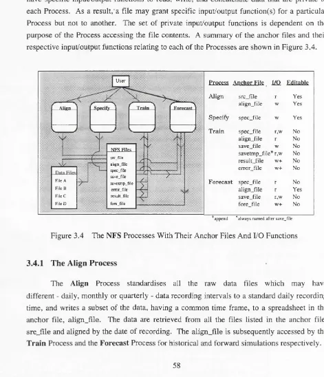
Process Design ... 58
3.4.1 The Align Process ... 58
3.4.2 The Specify Process ... 59
3.4.3 The Train Process ... 59
3.4.4 The Forecast Process ... 60
Summary ... 61
Implementation Of Neural Forecasting System
System Overview ... 634.1.1 The Mc/itt Module ... 64
4.1.2 The I/O Module ... 64
4.1.3 The Module ... 65
4.1.4 The Load Module ... 65
4.1.5 Tht Backpropagation ModMlt ... 66
Data Alignment ... 66
4.2.1 Common Time Frame ... 67
4.2.2 Common Recording Time ... 67
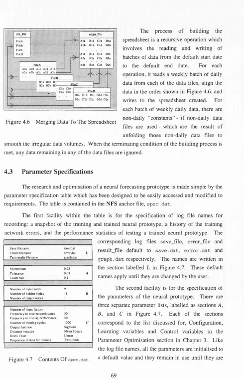
4.2.3 Data Merging ... 68
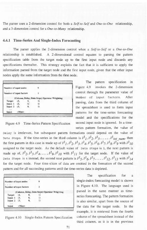
Parameter Specifications ... 69
Pattern Specification Language ... 70
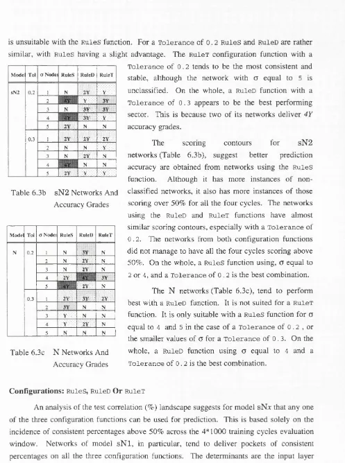
4.4.1 Time-Series And Single-Index Forecasting ... 71
4.5 Snapshot Facility ... 72
4.6 Summary ... 74
Chapter 5 Experimental Strategy
5.1 Neural Time-Series Analysis ... 755.1.1 Notations ... 75
5.1.2 Experimental Data ... 77
5.2 Data Form Of The Index ... 80
5.3 Optimisation Of Neural Forecasting Models ... 81
5.4 Adaptation Of Optimised Networks ... 84
5.5 Summary ... 85
Chapter 6 Performance Analysis
6.1 Raw Data Form ... 876.2 Network Optimisation ... 88
6.2.1 Correlation Measurement ... 89
6.2.2 Prediction Accuracy ... 90
6.2.3 Curve-Fitting ... 92
6.2.4 Optimum Network ... 96
6.3 Adaptation ... 102
6.3.1 Similar Data Trend ... 102
6.3.2 Dissimilar Data Trend ... 105
6.4 Summary ... 108
Chapter 7 Assessment
7.1 Targets Review ... I l l 7.2 The RTPI Indicator ... 1127.3 Network Generalisation ... 116
7.3.1 Global Minimum Error ... 116
7.3.2 Neural Learning And Extrapolation ... 118
7.4 Forecasting And Using A Forecast ... 119
7.4.1 Evaluation Window: Static vs Dynamic ... 119
7.4.2 Investment Strategy Formation ... 120
7.5 A Forecasting Tool ... 122
7.5.1 Model sNx vs Related Neural Systems ... 122
7.5.2 Neural Forecasting vs Traditional Forecasting ... 123
7.6 Summary ... 124
Chapter 8 Conclusion And Future Work
8.1 Summary ... 1278.2 Research Contributions ... 130
8.3 Future Research ... 131
References ... 135
Appendix A Processes Of The Neural Forecasting System ... 141
Appendix B Correlation Measurements From Experiment 2(a)(1) To 2a(iii) .... 147
Appendix C Prediction Accuracy Of Rules Networks ... 153
Appendix D Prediction Accuracy Of RuleD Networks ... 157
Appendix E Prediction Accuracy Of RuleT Networks ... 161
Appendix F sNl Networks And Relative Threshold Prediction Index ... 165
Appendix G sN2 Networks And Relative Threshold Prediction Index ... 171
List Of Figures
Figure 1.1 Figure 2.1 Figure 2.2 Figure 2.3 Figure 2.4 Figure 2.5 Figure 2.6 Figure 2.7 Figure 3.1 Figure 3.2a Figure 3.2b Figure 3.2c Figure 3.3 Figure 3.4 Figure 3.5 Figure 3.6 Figure 3.7 Figure 3.8 Figure 4.1 Figure 4.2 Figure 4.3 Figure 4.4 Figure 4.5 Figure 4.6 Figure 4.7 Figure 4.8 Figure 4.9 Figure 4.10 Figure 4.11 Figure 5.1 Figure 5.2 Figure 5.3 Figure 5.4 Figure 5.5 Figure 5.6 Figure 5.7 Figure 6.1 Figure 6.2a Figure 6.2bComputation Of A Simple Node ... 14
Some Basics Of Candle Chart Lines And Indicators ... 31
The Simple Linear Regression Model ... 34
Rule Sets For A Technical Trading System ... 36
Elements Of Elliot Wave Theory ... 37
Portfolio Selection By MPT ... 39
Processing Knowledge For The Qualification Of Expertise ... 42
Rule Sets With Symbols Processed Dynamically ... 45
Definition Of The Direction Of Movement ... 55
Correlation Of Forecast By v c o rr Definition ... 56
Correlation Of Forecast By DCorr Definition ... 56
Correlation Of Forecast By VDCorr Definition ... 56
Definition Of Unrealisable Weighted Return ... 57
NFS Processes With Their Anchor Files And FO Functions ... 58
A Structure Chart For The Align Process ... 143
A Structure Chart For The Specify Process ... 144
A Structure Chart For The Train Process ... 145
A Structure Chart For The Forecast Process ... 146
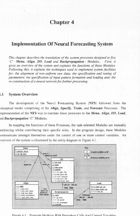
Program Modules With Procedure Calls And Control Variables ... 63
Definition Of Default Start Date ... 67
Definition Of Default End Date ... 67
File Layouts Of Recording Times ... 68
Calendar For Unfolding Data ... 68
Merging Data For The Spreadsheet ... 69
Contents Of sp ec. d a t ... 69
Pattern Specification Language ... 70
Time-Series Pattern Specification ... 71
Single-Index Pattern Specification ... 71
Multi-Index Pattern Specification ... 72
Types Of Pattern Formations In A Consolidation Trend ... 78
A Bull Trend ... 78
A Recovery Trend ... 78
Specifications For Experiment 1 80 Specifications For Experiments 2al(i)-2al(iii) To 2a3(i)-2a3(iii) 82 Specifications For Experiments 2bl(i) -2bl(iii) To 2b3(i)-2b3(iii) .... 83
Specifications For Experiments 3a(i) And 3a(ii) ... 84
Logarithmic vs Linear Inputs ... 88 Test Correlation (%) For Rules Configuration Function And
Tolerance = 0.02 155
Test Correlation (%) For Rules Configuration Function And
Figure 6.3a Test Correlation (%) For RuleD Configuration Function And
Tolerance —0.02 159
Figure 6.3b Test Correlation (%) For RuleD Configuration Function And
Tolerance *= 0.03... ... 160
Figure 6.4a Test Correlation (%) For RuleT Configuration Function And Tolerance = 0.02 ... 163
Figure 6.4b Test Correlation (%) For RuleT Configuration Function And Tolerance = 0.03 164 Figure 6.5a RTPI Of s N l Networks With Configurations Using
a
= 1 167 Figure 6.5b RTPI Of s N l Networks With Configurations Usinga
= 2 167 Figure 6.5c RTPI Of s N l Networks With Configurations Usinga
= 3 168 Figure 6.5d RTPI Of s N l Networks With Configurations Usinga
= 4 168 Figure 6.5e RTPI Of s N l Networks With Configurations Usinga
= 5 169 Figure 6.6a RTPI Of sN2 Networks With Configurations Using o = 1 173 Figure 6.6b RTPI Of sN2 Networks With Configurations Usinga
= 2 173 Figure 6.6c RTPI Of sN2 Networks With Configurations Using G = 3 174 Figure 6.6d RTPI Of sN2 Networks With Configurations Using 0 = 4 174 Figure 6.6e RTPI Of sN2 Networks With Configurations Using o = 5 175 Figure 6.7a RTPI Of N Networks With Configurations Using o = 1 179 Figure 6.7b RTPI Of N Networks With Configurations Using o = 2 179 Figure 6.7c RTPI Of N Networks With Configurations Using 0 = 3 180 Figure 6.7d RTPI Of N Networks With Configurations Using 0 = 4 180 Figure 6.7e RTPI Of N Networks With Configurations Using 0 = 5 181 Figure 6.8 Candidates For Optimum Network Of Model s N l ... 97Figure 6.9 Candidates For Optimum Network Of Model sN2 ... 98
Figure 6.10 Candidates For Optimum Network Of Model N ... 99
Figure 6.11 Performnace Of Optimum Networks Selected For Models sNjc And N ... 100
Figure 6.12a Forecasts On Tnp/e-Top Pattern By Optimum s N l Network ... 100
Figure 6.12b Forecasts On Tnp/e-Top Pattern By Optimum N Network ... 101
Figure 6.13 Optimum Networks Forecasting On Double-Top Pattern ... 103
Figure 6.14 Optimum Networks Forecasting On Narrow Band Pattern ... 104
Figure 6.15 Optimum Networks Forecasting On Bull Trend Pattern ... 106
Figure 6.16 Optimum Networks Forecasting On Recovery Trend Pattern ... 107
Figure 7.1 Forecasts And Correct Correlations On Test Data Of Double-Top Psiiitm ... 120
List Of Tables
Table 2.1 Hog Prices vs Hog And Cattle Slaughter... 29
Table 6.1 Correlation Measurements From Experiments 2a(i) To 2a(iii) ... 149
Table 6.2 Prediction Accuracy And Weighted Return By vcorr, DCorr And VDCorr 89 Table 6.3 s N l Networks And Accuracy Grades ... 90
Table 6.3b sN2 Networks And Accuracy Grades ... 91
Table 6.3c N Networks And Accuracy Grades ... 91
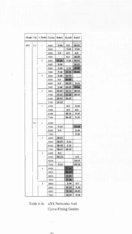
Table 6.4a s N l Networks And Curve-Fitting Grades ... 93
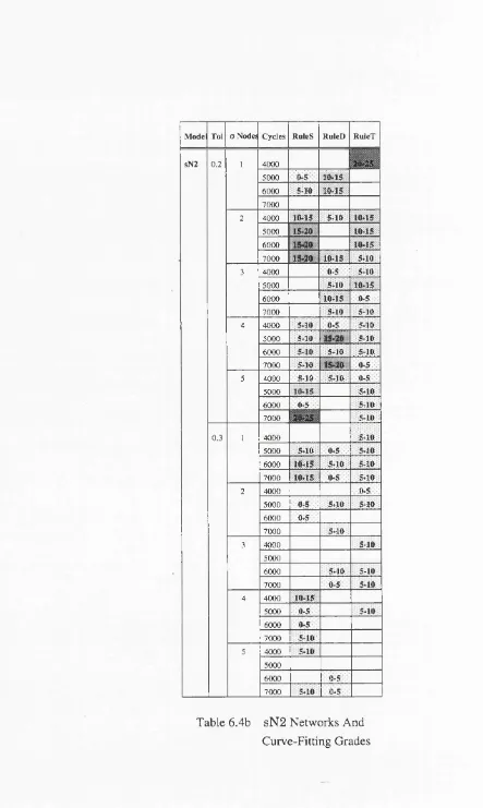
Table 6.4b sN2 Networks And Curve-Fitting Grades ... 94
Table 6.4c N Networks And Curve-Fitting Grades ... 95
Table 7.1 RTPI And Accuracy Below The 50% Threshold ... 113
Table 7.2 RTPI And Accuracy Equal To The 50% Threshold ... 114
Table 7.3 RTPI And Accuracy Above The 50% Threshold ... 114
Table 7.4 Average Network Errors And Forecast Performances ... 117
Chapter 1
Introduction
This chapter presents the motivations, aim, and contributions o f this thesis. Initially, it states the properties o f neural networks that motivate this research. There is then a survey o f financial neural forecasting, emphasising research systems applied to **real-world'* data. Next, it presents the aim o f the thesis, the objectives o f the experiments undertaken, and the choice o f specific pattern features chosen for the experimental data sets. Finally, it gives an overview o f
the thesis contribution and organisation.
1.1
Motivations
Neural networks have great potential for discovering the underlying structure of non-linear time-series and extrapolating these time-series to the future [LapFar88, ShaPat90, TanAlm90, MarHil91, SriLoo91]. In contrast, traditional statistical methods [HanRei89] are restrictive as they try to express these non-linear relationships as linear models. Dutta and Shekar [DutShe88] confirmed this in their comparison studies, neural networks consistently out-perform multi-regression models for predicting bond ratings: the former averaging at 80% accuracy against 60% by the latter. In addition, Chakraborty et al [ChaMeh92] showed their neural multi-index model approximates flour prices significantly better, providing a better fit for the test data than Tiao and Tsay’s auto-regressive moving average model. Latterly, these optimistic views have been reinforced by Schonenberg [Schone90] who obtained 90% accuracy for forecasting stocks.
N - \
1=0
Figure 1.1 Computation Of A Simple Node
Artificial neural networks are mathematical models of simulated neurons based on our present understanding of the biological nervous system. The characteristics of the well-studied models, for example the Backpropagation model, ART, the Perceptron, Self-Organising Maps are well documented [Lippma87, Wasser89, Dayhof90, HerKro91]. Typically, a neural network like that of a Backpropagation model is composed of a number of processing elements (nodes) that are densely interconnected by links with variable weights. Unlike conventional sequential processing, all the adjacent nodes process their outputs in parallel. Each node delivers an output, y according to an activation rule. In its simplest form, the rule for a non-linear output of a node is a sum of its N weighted inputs as shown in Figure 1.1. The transition function,/, normally has a binary, linear, sigmoid or hyperbolic tangent characteristic. As a result, a neural model is made unique by the specifications of the topology and dimension of the network, the characteristics of the nodes including the type of transition function used, and the learning algorithm.
1.1.1 Forecasting Research Approaches
In his report on neural learning procedures, Hinton [Hinton87] classified neural research into three main categories: search, representation and learning. - The investigative procedure carried out in the first category searches the weight space for an optimal solution to the network mapping in a constraint-satisfying manner. In the second, the research focuses on identifying the physical representation of the inputs that best represents the salient features of the domain. Finally, in the learning category, the research estimates a learning algorithm modelling the relationships of all the network elements to present a mapping solution in some numeric form.
more (multivariate) independent variables and to use the learnt interdependencies for prediction.
From the point of view of neural computing, neural forecasting research could, therefore, be viewed as a concentration of efforts in any one of the three neural categories applied to either one of the forecasting methods using a specific set of financial data for analysis. Of the three choices, the most popular approach has initially been the exploitation of the unique learning ability of a neural model on a specific forecasting application. To date, the Backpropagation model has always been the model of choice, mainly because it has been widely researched and the supervised learning strategy is well-suited for the task.
For instance, Schonenberg [Schone90] carried out time-series forecasting research on German stocks by experimenting with four different neural models, Adaline, Madaline, the Perceptron and Backpropagation. In his approach, he had taken to optimising the models’ networks with regard to learning the features of each of the different types of stocks. He was able to isolate and differentiate the behaviour of the models by fine-tuning neural parameters such as the size and the types of input of the input vectors, the ways of splitting the input vectors and the network configuration.
Varfis and Versino [VarVer91] like Schonenberg used a Backpropagation model for univariate forecasting. One of the areas on which they concentrated was the input data and the structure of the input vectors. Their main concern was the simulation of the underlying features of seasonal behaviour and time lags in an otherwise “fiat” network.
Unlike Schonenberg, or Varfis and Versino, who used different time-series information derived from one specific type of price index for inputs to the neural model, there are others like Kimoto and Asakawa [KimAsa90], and Windsor and Harker [WindHar90] who have used a neural model for multivariate forecasting. Kimoto and Asakawa, for example, developed a prediction system for the Japanese stock index, TOPIX, using clusters of Backpropagation networks. Each cluster in the network is responsible for a batch of indices and macro-economic data, and all the outputs are combined to produce a weighted average for the weekly returns of TOPIX. In addition to optimising the network, they also modified the learning algorithm to improve the speed of training. The supplementary learning process is one such enhancement. It is a control applied to each training cycle to ensure a training pattern would not be unnecessarily presented for further training once the pattern has been sufficiently learnt. The learning criteria is based on the dynamic minimum network error achieved in the mapping.
movements of the indices as a whole. Apart from that, they also investigated ways to bring out the structure of the training data. To do so, they focused on methods for representing the data. They transformed the actual input values to fit logarithms onto a regression line using an equation which they derived. As a result, their system predicted the deviations of the Index from the exponential growth instead of its absolute value.
The papers by Refenes [Refene91], and Jang and Lai [JanLai93] are examples of approaches by learning. Refenes’ CLS+ model forecasts the Deutschemarks by dynamically updating the dimension of the hidden nodes using the constructive learning procedure. The model is supported by a linear classifier which can be trained to optimise the errors between its output and the target. As it is, a training session always commences with a one hidden node network. This is followed by a look ahead test procedure to establish whether there would be a reduction in the errors by an additional linear classifier. An affirmative result would have the dimension of the hidden layer increased and the weights of the linear classifier frozen. The test procedure is repeated for further additional classifiers until an optimal configuration is obtained.
Jang and Lai, who found the fixed-structure Backpropagation model too rigid, developed the DAS net to synthesise and adapt its topology for Taiwanese stocks. The net is a hierarchy of networks representing both the short- and long-term knowledge of a selection of technical indices. The short-term knowledge is used for short-term prediction, principally for trading decision making. In addition, it supplements the knowledge for the long-term view as the time window advances. Together, these two levels of knowledge control the continuous self-adjustment of the network’s assessment of curve-fitting.
Yet another variant of the learning approach is to explore the characteristics of the nodes as [Casdag89] and [JonLee90] have done. They, like Jang and Lai [JanLai93], redressed the fixed-structure problem with radial basis functions (RBF). The research on this alternative tool is concerned with the representation of the hidden layer and its evaluation. The composition of an RBF network is a number of RBF nodes evaluating a Gaussian-like kernel function, and because it is designed to use a minimum hidden layer dimension, it is claimed to offer a better network generalisation. Another of its advantages is that the layers of the network can be trained independently on a layer by layer basis. This is a sharp contrast to the usual method of computing each node and expanding it across the layers of the network, or incrementally like CLS+.
2-dimensional “flat” network. This is an inconvenience which Varfis and Vesino tried to simulate by aligning data from more than one recording time alongside each other as inputs to a 2-dimensional input vector. Others like Kamijo and Tanagawa [KamTan90], and Wong [Wong91] tried to redress the issue explicitly by adapting the framework of the network itself.
In the case of Tanigawa and Kamijo [KamTan90, TanKam92], the authors used a recurrent neural network for the recognition of candle chart patterns (discussed in Chapter 2). Effectively, a recurrent network [WilZip89] is a generalised Backpropagation model with a new learning algorithm capable of retaining temporal information. The recurrent learning procedure uses the information that has been accumulated in the memory which can either have a fixed or indefinite historical span. In [TanKam92], the proposed extended Backpropagation network had two hidden layers. Each of these was divided into two sets of units, for holding the stock prices and for the corresponding temporal information about its previous activity. Its successes in recognising a triangle chart pattern resulted in a Dynamic Programming matcher being incorporated into a new version of the system. The matcher is designed to resolve non-linear time elasticity (a feature of charting where the pattern could be formed but could have variable window sizes).
Wong [Wong91] introduced time by the addition of a third dimension to a neural model. Unlike [TanKam92]’s 2-dimensional temporal network which simulates time by splitting the hidden layers into two halves, the NeuroForecaster simulates time orientation by concatenating duplicates of an entire 2-dimensional network to form a single network. This extensive network is burdened by long network training. Subsequently, the FastProp learning algorithm [Wong91] was introduced to improve the rate of convergence. It trains sections of the network and clusters them according to the ranking of the Accumulated Input Error index. The index is built with a strategy to rank the data from an entire time-series to several clusters according to the dynamic causal relationship between the input data and the output.
Despite the various efforts made to enhance the standard Backpropagation model for forecasting with non-linear inputs, Deboeck [Deboec92], being a financial player, called for attention to an approach that is feasible but yet often overlooked. He asserted that in order for financial systems to benefit from neural processing, it is more important to concentrate on the basics of the application domain rather than the network paradigms. Areas suggested are those relating to the dynamics of the domain such as the pre-processing of input data, risk management and trading styles.
1.2
Thesis Aim
The AIM of this thesis is to investigate the use of the Backpropagation neural model for time-series forecasting. A new method to enhance input representations to a neural network, referred to as model sNx, has been developed. It has been studied alongside a traditional method in model N. The two methods reduce the unprocessed network inputs to a value between 0 and 1. Unlike the method in model N, the variants of model sN%, sNl and sN2, accentuate the contracted input value by different magnitudes. This approach to data reduction exploits the characteristics of neural extrapolation to achieve better prediction accuracy. The feasibility of the principle of model sNx has been shown in forecasting the direction of the FTSE-100 Index.
The experimental strategy involves optimisation procedures using one data set and the application of the optimal network from each model to make forecasts on different data sets with similar and dissimilar pattern features to the first.
Experimental Objectives
The objectives of the experiments for optimisation were: (1) To select a suitable raw data form.
Either the ogarithmic or linear (absolute value) data form is selected as more suitable for inputs to an NFS (explained in Section 1.3) configured network. This also serves to justify the research approach for this thesis. The better data fdrm was applied to the rest of the experiments.
(2) To select a suitable prediction accuracy measurement.
A prediction is accurate if the direction of a prediction correlates with the tracking data. A data correlation can be defined by value, direction, or value and direction. A forecast value for tomorrow is correct according to interpretation by: value, if the movement of the forecast value compared with today’s tracking value is the same as the movement of the tracking data, from today to tomorrow; direction, if the direction of the forecast movement from today to tomorrow correlates with the movement of the tracking data at the same period; value and direction, if the interpretations for each of the separate elements are combined. The best interpretations are subsequently used for evaluations of other objectives.
(3) To select a suitable configuration function.
Each of the three function values were combined with a set of five different I values to configure a group of networks as contenders for an optimal network to represent models N and sN%. The test cases were cross-validated with the tolerance value. (4) To select the better version of model sNr.
The better version, either s N l or sN2, forecasting with a more consistent manner across the group of test cases, is selected.
An optimal network selected for each model, sN r and N, is like the selection in (4), characterised by consistency, a gently rolling prediction accuracy landscape across the section of the evaluation window without intermittent spurts of exceedingly good accuracy.
The objective of the experiments applying the optimised networks was:
(5) To observe the optimised network accommodating to new data sets.
The double-top pattern (explained in the section on Experimental Data below) was applied, in part, to test the networks’ ability to adapt to a new data set similar to one on which it was optimised. Like the other experimental patterns, it was used to test the optimised network’s performance on specific pattern features.
The evaluations for objectives (3), (4) and (5) were based on a combination of performance statistics, among them being, the test correlation (%), the corresponding weighted return (%), the RTPI indicator (explained in Section 1.3) and the forecast error margins. The test correlation percentage is the prediction accuracy percentage measured for the test data set. The weighted return percentage is the final total of the number of Index points made or lost, as points amounting to the size of the movement are added whenever a forecast correlates and subtracted when it does not. It is an indirect indication of a network’s ability to forecast the salient movements of the test pattern. The RTPI indicator is developed to combine these two measurements to differentiate the forecasting performances of networks. A minimum accuracy of 50% was assigned to the interpretation of a “weak” performance and a “weak” network is differentiated by a negative RTPI value as opposed to the positive valued “good” network.
The effectiveness of a neural forecasting tool is discovered by appraising the neural forecasting results in a practical situation, highlighting its usability and areas for improvement.
Experimental Data
The experimental data sets were selected from historical periods showing three data trends: consolidation (“non-diversifying” pattern), bull (“rising” pattern) and recovery
because its data values fluctuate consistently within a relatively smaller range of values, therefore being particularly suitable for training and testing. As a result, three different
consolidation patterns were used, triple-top, double-top and narrow band, in addition to the
bull and recovery patterns. Each of these patterns have distinctive observational features: (a) triple-top.
Its signature is three almost identical peaks. The data values across the time window lie neatly within fixed upper and lower bounds. The test pattern comprised a peak formation. It was used for the optimisation procedures.
(b) double-top.
Its signature is two. rather than three peaks. Some of the data values in the second peak are slightly outside the upper bound of the first. This section is part of the test pattern.
(c) narrow band.
Its signature is data modulating within a tight range. An additional and interesting feature is a breakout, a sudden diversification with a rising pattern at the end. The major objective is forecasting the breakout section whose data values are outside the range on which the network has been trained.
(d) bull.
Its signature is a rapidly rising pattern followed by a loss in momentum with the trend “moving sideways”. The emphasis is on the behaviour of a network trained on a rising pattern and tested on a consolidation pattern trend, with some of the data values outside the training range as well.
(e) recovery.
Its signature is a rising pattern followed immediately by a sharp plunge and a gradual recovery from the dip. The recovery test pattern is similar to the rising pattern of the training pattern, but they do not lie within the same range of values.
1.3
Thesis Contributions
The thesis contributions may be listed as follows:
(a) A good input representation for data reduction.
It has been proven that the new method of enhancing input, reducing it to values between 0 and 1, is better than the commonly used formula. The method in model sN r triumphs over model N in the following ways:
♦ a more stable prediction accuracy, offering more consistent percentages across. a section of training cycles.
♦ a better corresponding weighted return percentage, indicating the network’s ability to forecast better defined data movements.
♦ smaller forecast error margins, overall.
♦ better adaptation to time and data changes, maintaining equal or higher prediction accuracy, with usually a slightly better return percentage and generally smaller forecast error margins.
(b) A neural forecasting indicator, the RTPI.
The Relative Threshold Prediction Indicator (RTPI) differentiates the forecasting capability of a network. A network’s forecasting capability is measured by its percentages of prediction accuracy and weighted return. The latter is the final total number of Index points made on the basis that if a forecasts correlates correctly, the size of the movement is added to the subtotal but it is deducted if it is incorrect. The RTPI indicator value differentiates a network forecasting below a specified prediction accuracy percentage by a negative indicator value and a positive value if it is above. Proofs of the principle in simulations showed the indicator is particularly useful in neural forecasting research as test cases are quite often large.
(c) A solution to forecasting during the c o n s o lid a tio n trend.
The consolidation trend occurs frequently and more persistently than other data trends. It is a situation where traditional methods, such as moving averages, the RSI indicator, or Elliot Wave Theory are not good as forecasts are “flat” and do not provide any lead. The principle of neural processing offers flexibility in designing neural outputs. Simulation studies using three different pattern formations in a
consolidation trend show it is possible to predict the direction of data movement, a small piece of information that could be exploited during a low risk period.
rather than time-varying conditions. An effective neural forecasting system should be able to do the following:
♦ Handle out-of-range problems.
An effective neural forecasting tool for non-linear data should not only forecast within a specific range of data values. It must be able to handle forecasting data values that are beyond the boundaries of the training data set.
♦ Handle forecasting reliability.
The confidence on a neural forecast is unknown and it is not easily measured. This problem can be resolved by two approaches: to research a confidence indicator and to research a more reliable and stable neural forecasting model across non-linear data. ♦ Handle intra-time-series information.
A neural forecast on the direction of a data move is not informative. It requires information about the forecast and the other data in the time-series. A neural forecast could be augmented by endogenous information. Information, such as projections of the following day’s high and low data values, provide cues for implementing a better investment strategy.
♦ Handle structured design for neural forecasting models.
Neural forecasting has been studied on an ad hoc basis using snapshots of a static time window. An effective neural forecasting model should handle the “generators” in the data that are responsible for the non-linear data movements. The implementation of the dynamics of the non-linear data forms a principled basis for designing an effective neural forecasting network.
In addition, the thesis has established the suitability of forecasting the FTSE-100 Index, on the Neural Forecasting System (the NFS is explained below), with regard to:
(e) The raw data form.
It confirmed a linear rather than a logarithmic data form is more suitable for forecasting, at least on the Backpropagation model of the NFS.
(f) The measurement of prediction accuracy.
It confirmed the best method to measure that a forecast has correctly correlated with the tracking Index is by the measurement method of value as opposed to direction or
(g) The dimension of the hidden layer, H.
It confirmed that H for a noisy data pattern, the triple-top, should be based on the configuration function with (j) equal to 2.
Finally,
(h) The Neural Forecasting System.
The NFS is specially developed to facilitate neural forecasting research and operational use. The system facilities are:
♦ Raw data integrity.
The problems of those raw data files which might have data with various sampling intervals and differing data volumes are solved by standardising to a daily sampling interval and merging by date into a spreadsheet for subsequent use.
♦ A neural parameters specification table.
The table allows easy access to all the modifiable neural and system control parameters as a system file. It contains: names of log files, learning parameters, training control parameters and the specification language.
♦ A forecasting model specification language.
The language allows the specification for time-series, single-index or multi-index forecasting. It has parameters to specify: a weighting for the input value according to the arithmetic operator specified; a time lag or advance in relation to the target node input; the omission of specific time slices of data forming successive input patterns. ♦ Reconstruction of network.
A snapshot facility records an image of the training network at regular intervals. A recorded image allows the re-construction of a partially trained network for continuation or extension of a training session, or the re-construction of a trained network for forward simulation.
♦ Options for forecasting simulations.
It offers options for historical and forward simulation which are accessible directly via menu selections. The historical simulation option undertakes to train and test a prototype neural model specified in the parameter specification table. The forward simulation option delivers a forecast value for one day ahead using a re-constructed trained neural network. The forecast is for testing on live data.
♦ User support.
1.4
Thesis Organisation
Following the Japanese New Information Processing Technology research programme [MITI90], there is a proposal for the next generation of intelligent systems using “soft” logic and “hard” logic. Both models of computation embrace a spectrum of state-of-the-art intelligent techniques. There are, on the “soft” side, techniques like expert systems, neural networks, genetic algorithms, fuzzy logic [TreLoo90, TreGoo92]. The complementary tools of “hard” logic such as parallel computers and silicon chips are usually used to support the computations of the “soft” techniques.
Chapter 2 exemplifies the significance of “soft” logic for financial systems. Initially, it surveys the classical forecasting methods to highlight their shortcomings. Following that, there is a description of the practical use of the “soft” neural network for sub-symbolic processing. Financial adjectives like increasing and bull which are not easily measured are qualified from time-series data. They are then asserted as facts in the knowledge-base for evaluation in a financial rule-based system.
The description of the research commences with Chapter 3, which reports the development of the customised Neural Forecasting System. Initially, it describes the system specifications, with outlines of general requirements, such as the operating platform, the user interface and the system characteristics. Following this are the technical requirements with details of the Backpropagation model and the research facilities needed to facilitate neural forecasting. Lastly, it explains the system design, with outlines of the system processes mapping these specifications.
Chapter 4 describes the translation of the system processes designed to five ‘C’ - Menu, Align, I/O, Load and Backpropagation - Modules. First, it gives an overview of the system and explains the functions of these Modules. Following this, it explains the techniques used to implement system facilities for: the alignment of non-uniform raw data; the specification and tuning of parameters; the specification of input pattern formation and loading; and the re-construction of a neural network for further processing.
Chapter 5 reports the strategy used to validate the data reduction method in model sNx. Initially, it explains the notations used, including the RTPI indicator, the method of extrapolation, and the choice of data sets. Thereafter, it describes the experiments - to select a suitable raw data form, optimisation of network configuration and neural parameters to identify a suitable prediction accuracy measurement, and testing the optimised networks on time complex data sets - and evaluation criterion.
and the better of models s N l and sN2. The evaluation discusses, amongst other things, the test correlation (%), its weighted return (%) and the RTPI indicator.
Chapter 7 assesses the feasibility of neural forecasting, reviewing their effectiveness to deliver consistently good results and as a usable tool. First, it examines the RTPI
indicator to justify its achievements and relevance. Thereafter, it examines the measurement of network generalisation and the relationship between network learning and extrapolation. Next, it examines the usability of neural forecasts to form investment strategies, and, finally, it compares model sNx with related work and other forecasting tools.
Chapter 2
Soft Logic And Finance
This chapter exemplifies the significance o f “soft*’ logic for financial systems. Initially, it surveys the classical forecasting methods to highlight their shortcomings. Following that, there is a description o f the practical use o f the “soft” neurçil network for sub-symbolic processing. Financial adjectives like “increasing” and “bull” which are not easily measured are qualified from time-series data. They are then asserted as facts in the knowledge-base for evaluation in a financial rule-based system.
2.1
Financial Forecasting
Due to the Darwinian nature of operations in the financial markets, every investment strategy is made with a sound money management policy. However, the volatile atmosphere dictates that the decision of a strategy is made preceding the decision of the policy, following a thorough evaluation of the market. A speculator will aspire to make a profit by taking advantage of the results of the evaluation, which is, speculating the movements of the market data. Apart from speculating to be successful, an even greater temptation for the speculator is the prospect of capital gains by a “low risks and high rewards” approach. Consequently, they are increasingly turning to the latest technology for competitive solutions to their optimisation and forecasting problems.
In a quantitative approach, the manipulation and analysis of the data is carried out as an extrapolative (time-series) model or a causal (econometric) model. The choice is dependent on circumstances and the usage of the forecast, A time-series model is selected for prediction by applying the value of a variable and extrapolating the past values of the same variable. By contrast, a causal model is used for prediction by applying the value of a dependent variable and identifying its causal relationships with the values of other independent variables. In either case, the techniques used for forecasting fall into three analytical categories, fundamental analysis, technical analysis, and quantitative analysis.
Fundamental analysis is to find speculative opportunities from economic data by identifying potential major shifts in trends in the balance of the market supply and demand.
Technical analysis is to speculate on the supply and demand of the market based on the assumption that the market moves in cycles and there is repetition of its trend as patterns in price charts.
Quantitative analysis is to speculate by formally constructing a market model and computing an efficient frontier which would offer a maximum reward according to the amount of risk that is to be taken.
2.1.1 Fundamental Analysis
The core activity of fundamental analysis is to assess the trends of corporate profits and to analyse the attitudes of investors toward those profits with a focus on the supply and demand pattern. The information used is often derived from a range of marketing figures that are thought to influence the product or financial instrument being analysed. Amongst the figures normally studied are economic data - the gross national product, the balance of payment and the interest rates - corporate accounting reports, and currency rates. The methods used to uncover the supply-demand trend do not normally analyse the prices directly. Instead, there are analyses of the trends made by prices and those market variables that influence the direction of the trends. The variables incorporated in such analyses would often include seasonal influences, inflation, market response, government policies and international agreements. The opinions derived from these fundamentals are normally used to influence the medium to long term policies of future investments.
Old Hand Approaches
Tabular And Graphic Approaches
The tabular and graphic (TAG) approach is a systematic way to examine a balance table for the relationship between the supply and depreciation statistics of prices. To illustrate the approach, the balance table in Table 2.1 is a simple model to project hog prices. The columns of data reflect the relationship between the slaughter levels and the price of hog for contracts to be delivered in June for each of the years tabulated.
It is obvious from the table that there
Year
Dec May Slaughter (1000 head) Dec-May
Avg Price June Hogs
4- PPI* (cents/Ih)
Hog Cattle
1976 21,137 25 9
1975 • 19,324 2 6 1
l i i l i l i i i l i i i i i 20,295 22.9
1977 20,641 30,5
1973 40,292 16,889 26.6
1974 41,184 17,230 27.0 .
17,264
1972 45,102 17,443 23,3
1981 47,479 17,063 17.9
1971 49,087 17,318 17 7
49,286 16,284 15 3 ...
Product Price Index
Table 2.1 Hog prices vs Hog And Cattle Slaughter'""""'
is a correlation between the high prices of hog and its slaughter levels. However, it appears that the prices in the shaded band, are relatively low when they are compared to the other years. An explanation for this might have been that prices were competitively set to offset an influx of alternative meat supply shown by the high increase of cattle slaughter for the same period. In addition, it is noticeable that for 1974 and 1979, there are similar levels of hog and cattle slaughters, and yet the prices of hogs are much higher in 1974. Again, there are such similar slaughter levels and prices differences for 1971 and 1980, and 1972 and 1979. This observation suggests that there is a trend for the price of hogs to fall in the latter years and it could possibly be due to a shift in the consumption of red meat.
This simple model highlights three possible variables that can determine the prices of hog: hog slaughter, cattle slaughter and time. In addition, it shows the projection of the market for hogs by applying marketing knowledge to the analysis of a selected set of historical information. Following this simple example analysis, it is clear that the TAG approach could not be made to work well if the explanations of price fluctuations are due to more than one factor. This view is also consistent with Remus’ [Remus87] report on the relative impact of tabular and graphic displays for decision making. His investigations showed that tabular displays are, by far, more suitable for decision makers to weigh the appropriate factors in low complex problems. By contrast, graphical displays also play a significant role up to an intermediate level of environmental complexity. It is therefore, not surprising that in real situations where multiple factors can be involved, the TAG approach becomes a cumbersome forecasting tool. When such a situation arises, it is not unusual to formalise the TAG approach with a more efficient mathematical approach like regression analysis.
As an example, the TAG relationships for the December to May hog analysis can be translated to a linear equation like,
P ^ a + bjH + b2C + b^T (2.0)
where P is the average price of June hogs divided by the PPI, H is the hog slaughter, C is the cattle slaughter, and T is the time trend. The regression equation (2.0) defines the price level,
P that corresponds to any combination of hog and cattle slaughters and time. The values of the regression coefficients <2, bj, ^3 can be determined by a multiple regression
model and subsequently substituted into equation (2.0) to obtain a price forecast for hogs. A discussion on the mathematics of multiple regression can be found in [Schwag85 and HanRei89] for example. A linear regression model is also outlined in the next section on Technical Analysis.
2.1.2 Technical Analysis
Unlike fundamental analysis, technical analysis is a study on the reaction of the market players to their assessments of any relevant market factors that can have an impact on the prices. It is based on the belief that the price chart is an unambiguous summary of the net impact of all fundamental and psychological factors, and that the major market turning points are the result of the market players themselves unbalancing the supply and demand equilibrium. This subject had evolved over a period of time into five main ways of analysing the internal structure of the market. They are, classical charting techniques, statistical techniques, mathematical techniques, system trading techniques, and behavioural techniques. Generally, these techniques are highly dependent on the vagaries of human behaviour and judgements on the common-sense forecasting principles on which these models are based.
Classical Charting Techniques
The art of speculation can be traced as far back as the sixteenth century, to the Japanese rice markets. These rice merchants had devised a method which is similar to the Japanese Candle chart technique to obtain insights of the market by representing prices as picturesque descriptions and interpreting them using ideas which are often criticised by forecasting sceptics as similar to practising folklore.
instances of candles with different shapes and sizes resulting in a variety of pattern formations. Each formation is recognised by a poetic description and any interpretation of its significance is based on myths surrounding the pattern. For example, the simple patterns on the top row of Figure 2.1 give a view of the general direction of the market based on the unique interpretation of the relationships of intra-day prices. They are then used as building blocks for more complex patterns like those along the bottom row. Each pictorial representation has a name which reflects its expected behaviour as it is told in folklore. The behaviour aspect is an important part of candle charting. It is an indication of the strategy to adopt in anticipation of the market behaving as predicted. For example, the formation of a window is to caution one to anticipate the “closing of the window” with an imminent change in the direction of the market. In the event of an unclosed window, it is a signal for the continuation of the present market trend.
Spinning Tops
0|Msn
W - — chwe
Doji Lines Umbrella Lines
$
gapf i l
gapDoji Star Shooting Star
window.
Window
Figure 2.1 Some Basics Of Candle Chart Lines And Indicators( N i s o n 9 ll
To obtain a current insight of the market, the price chart has to be reviewed constantly for the complete formation of any of the known candle patterns. In spite of this inconvenience, proponents believe that exploitation of the market is possible through the recognition of the known trends. As in candle charts, the western practise of charting is also concerned with the recognition of various descriptions of trend lines. Although the trend lines are derived from a different reasoning, they are equally mythical. Amongst the descriptions used are, head and shoulders, a triangle, an island reversal, and a double top.
Sources for further reading on charting are in [PringSO, Schwag85, Murphy86] and
[DunFee89, Nison91] for candle charts.
Charting techniques which rely on non-scientific general principles and which are entirely dependent on subjective interpretations do have their pitfalls. First of all, the
patterns formed in a non-linear chart may not be clear, as they are likely to suffer some degree of distortion due to time warp. As a result, all interpretations demand craftsmanship and even then they can be inconclusive. Even if a view is correct, this method of analysis is reactive, that is, by the time a trend line is recognisable as a result of the formation of a pattern, the speculator would only be able to speculate by reacting to the market situation and not so much as to exploit the market by anticipation. Despite such a major shortcoming, this technique has remained very popular and continues to be used especially to reinforce the views of some of the other techniques to be discussed later.
Statistical Techniques
Following the popularity of computers, statistical techniques have also become popular as a means to automate what is seen as a key element of charting, pattern recognition. Many statistical methods have been studied to formalise the common sense principles used by players in the market. Amongst the list of formulae studied to reflect the common principles used to explain the supply and demand of the market are: momentum, stochastic oscillator, moving averages, and Relative Strength Index (RSI). One of the goals of these methods is to turn an intra-day or daily price data into technical indicators that highlight certain aspects of the activity of the price. These indicators are to add precision and to eliminate some of the guesswork made to plot investment strategies.
The RSI indicator is a reading to compare the price at different times within the same chart. The calculation of the indicator to range from 0 to 100 uses the formula,
RSI^100-{100I <1 +RS>) (2.1)
where RS is the ratio of the exponentially smoothed moving average (EMA) of gains divided by the EMA of losses over a chosen time period, the tracking window. The dimension of the tracking window is one that is right and appropriate for viewing short, medium or long term charts.
In its simplest form, the indicator suggests an overbought market when the reading is above 70, and an oversold market when it is below 30. Such a reading merely indicates that the market trend is liable to see a short-term correction before too long. However, it is not a reliable indicator to signal buying or selling. At the most, an extreme RSI reading is a rather promising signal as it suggests that the market is likely to have to make a strong move to correct its present trend. When the correction has taken place, the main trend is also likely to follow the new direction for a while.
market low but not a lower RSI. The emergence of this market signal simply implies that there is a continuing supply by sellers which can mean that it is fairly probable that the price is likely to continue to go down. As a result, a positive divergence is interpreted as a buy signal and it has been found to be fairly reliable. In practice, the signal is always applied with consolidating evidence from other indicators. This is because the early onset of a divergence can indicate that the market can either diverge significantly to attain a lower low or it can also move but not too significantly from its current low position. A similar reasoning also applies to a negative divergence when the market is at its top end.
The reverse of a divergence, a convergence, is the situation when the RSI confirms the direction of the market by taking a new high or a new low. It is a sign to suggests that the market is likely to continue to follow its current trend, and like divergence, it is often applied with caution.
Like other technical indicators, the RSI has the ability to hint at an imminent market correction or a market trend. These signals are, however, often inconclusive and any potential misleading move has to be eliminated by other indicators and market opinions. In any case, making good decisions with it would require a substantial amount of practical experience. In the experimentation with other indicators, the RSI has been found to be useful with other techniques such as, the Elliot Wave Theory. A range of these popular techniques are sold as proprietary packages like Comtrend, TeleTrac and Tradecenter. They offer facilities for consultation with different methods within one price chart updated in real-time. It has the disadvantage for not allowing the technical indicators to be optimised as they are used in a model.
Mathematical Techniques
Uokoown true regressioB line
Conditional Distributions
Y = a + bX
Estimated regression line
*tt y 4» X ;
Figure 2.2 The Sinjpie Linear Regression Model
The simplest form of regression analysis is the simple linear regression of two variables. It is an optimisation method that finds a straight line that can best fit all the data points in the sample set. For example, if the dependent variable is symbolised by Y and the independent variable by
X, then the overall distribution of Y values is termed the marginal distribution. Then the distribution of Y for a given value of X is known as the conditional distribution for that particular value of X. In any simple regression problem, there is one marginal distribution and a number of different conditional distributions for each different value of X. As a result, to say that the relationship between Y and X is linear implies that the mean values of all the conditional distributions lie in a straight line which is known as the regression line of Y on X.
Referring to the example in the TAG approach, a simple regression model to express the measurement of the true regression line is,
P = a + bH (2.2)
where a is the estimate of the true intercept and b is the estimate of the true slope. The estimation of the best fit line usually uses the least square criterion to minimise the sum of the squares of the vertical deviations of each point from that line. The vertical deviations are in fact a measure of the errors in the dependent P, and it is squared to remove the relevance of points that lie above or below this best fit line. Minimising the squared vertical deviations in P produces the regression line P on H. Assuming that, (h],p]), (h2,P2)^ • •, ^6 the
data points in the sample set, then the squared vertical deviations.
SD= ^ { y . - a - b x . y
i = l
(2.3)
AzV x y - V x V y
is minimised with the regression coefficients, b = ^ and
(3 = —(Y x). By adapting the basic equations of (2.2) and (2.3), the method can be
n
applied for multiple independent variables and non-linear relationships between H and P, just like the ternary equation of (2.0).
standard deviation, implying that it is sufficient to apply a regression which is based on an overall estimate of the conditional probability rather than one using different estimates for different values of H. Secondly, by using the assumption that the conditional distributions are normal, the model is more likely to become invalid when the trend changes. As a result, these assumptions are rather inflexible for non-linear applications.
System Trading Techniques
On frequent occasions when the market volatility is high, it is not uncommon for financial players to succumb to the undesirable weakness of difficulty in isolating emotion from rational judgements. Emotions like fear, greed or stress are major factors which can impair prudence to cause investment damages.
Technical trading systems are serious attempts to simulate expert trading using a set of rigorously tested decision rules. They are often regarded as useful systems as they allow users to avoid using human judgements directly and the trading decisions can help to dampen the users’ emotions in stressful times. To automate any trading tactics, any suitable technical methods that can generate valid technical indicators are applied and they are then optimised to give valid trading signals. These are then incorporated as a set of favourable conditions to meet in the conditional parts of decision rules that are specifically for recommending a
“ BUY” or a “ SELL” signal.
A technical indicator that is widely used is the moving average (MA). It computes the forecasts by taking a fixed number of periods back from the current period and uses the arithmetic mean of-the values in these periods as the next forecast value. Assuming that P is the tracking window, the value of the FTSE-100 Index, for example, X/ of the current period f, then the forecast for the future period, X/+7 is,
X;+7 = [Xj + Xi_i + . . . + X/+7 .p] / P (2.4)
For any value of P chosen by the user, equation (2.4) smoothes out variations in the values of X. By the nature of the calculation in the equation, it is unfortunate that the resulting forecast for the next period lags behind by one time slice. As a result any significant changes in the values of the time-series can only be detected after a time-delay. Despite this sensitivity to f , the MA can be suitably adapted to monitor the trend of the day-to-day fluctuations of prices. In addition, it is particularly useful as a screening device where a number of charts can be efficiently scanned to spot sudden price changes, momentum variations, new highs or lows, or variations in relative performances.
Rule RI
IF the madcet is b e a r
AND the price crosses the short-term MA from below THEN flag a 'BUY' signal bül do not activate until
the price penetrates the short-term MA by twice the v o l a t i l i t y
Rule R l.l
IF the 'BUY' signal has been flagged AND the price has not penetrated the MA by
twice the v o l a t i l i t y {q t 10 minutes
THEN cut the 'BUY' signal
qualified when the price of the unit is less than the long-term MA. Conversely, it is a bull
market. In the rule set, the calculation of the long-term MA is to measure the underlying trend of the unit, while the calculation of the short-term MA, over a suitable smaller tracking window, is to measure the recent price movement of the unit seen over that time window. Given that the system has to trigger the Figure 2.3 Rule Sets For A Technical “b u y ” signal with a certain amount of
Trading System intelligence but without any judgmental input, an estimation based on twice the volatility is used as a conservative threshold to eliminate any false market moves.
The example outlined highlighted three weaknesses using a statistical measurement, like MA for technical trading systems. Firstly, as it has been mentioned earlier, the nature of the formula is such that the programming can only allow the system to perform based on information from the last market cycle. Consequently, a MA oriented trading system is unable to anticipate. It is reactive rather than proactive. Secondly, MA forecasts with a time lag, and is therefore insensitive to ranging markets. The fact is, markets are more often ranging then trending. As a result, the system can only perform very well for short periods when the market is more trending as opposed to ranging. Thirdly, the decision rules lack a dynamic learning ability to adapt to the current market sentiment and the state of the user’s balance account. This is partly due to the limitations of current technology and partly to the difficulty in computing some of the market factors in real-time. Even if it were possible to include some tangible factors (like a bear market) into the rules, their definitions are difficult and often inadequately defined for non-linear situations, so as to not allow the system to be flexible enough to perform satisfactorily. For instance, the conservative measure of twice the
volatility may well result in many good opportunities going amiss.
Behavioural Techniques