Scattering and Lens Rigidity

University of Pennsylvania

ScholarlyCommons

Publicly Accessible Penn Dissertations

1-1-2014

Scattering and Lens Rigidity

Haomin Wen

University of Pennsylvania, [email protected]

Follow this and additional works at:http://repository.upenn.edu/edissertations

Part of theMathematics Commons

This paper is posted at ScholarlyCommons.http://repository.upenn.edu/edissertations/1498

For more information, please [email protected].

Recommended Citation

Wen, Haomin, "Scattering and Lens Rigidity" (2014).Publicly Accessible Penn Dissertations. 1498.

Scattering and Lens Rigidity

Abstract

Scattering rigidity of a Riemannian manifold allows one to tell the metric of a manifold with boundary by looking at the directions of geodesics at the boundary. Lens rigidity allows one to tell the metric of a manifold with boundary from the same information plus the length of geodesics. There are a variety of results about lens rigidity but very little is known for scattering rigidity. We will discuss the subtle difference between these two types of rigidities and prove that they are equivalent for two-dimensional simple manifolds with

boundaries. In particular, this implies

that two-dimensional simple manifolds (such as the

at disk) are scattering rigid since they are lens/boundary rigid (Pestov--Uhlmann, 2005).

Degree Type Dissertation

Degree Name

Doctor of Philosophy (PhD)

Graduate Group Mathematics

First Advisor

Christopher B. Croke

Keywords

boundary rigidity, inverse problem, lens rigidity, Riemannian geometry, scattering rigidity

SCATTERING AND LENS RIGIDITY

Haomin Wen

A DISSERTATION

in

Mathematics

Presented to the Faculties of the University of Pennsylvania in Partial

Fulfillment of the Requirements for the Degree of Doctor of Philosophy

2014

Christopher Croke, Professor of Mathematics

Supervisor of Dissertation

David Harbater, Professor of Mathematics

Graduate Group Chairperson

Dissertation Committee:

Acknowledgments

I owe my deepest gratitude to my advisor, Professor Christopher Croke, for his

excellent guidance and patience. I can always receive constructive comments and

warm encouragements when talking with him. Without his guidance and persistent

help this dissertation would not have been possible. I would like to thank Professor

Herman Gluck for teaching me all the fundamentals of differential geometry and

topology, creating excellent atmosphere for doing research. I would like to thank

Professor Wolfgang Ziller and Professor Dennis DeTurck for helping me to develope

my background in Geometry.

I would like to thank my friend Tong Li. I got many useful feedbacks when

showing my ideas to him. The topic of this dissertation originated from a discussion

with him.

I would also like to thank my parents. They were always encourging me to chase

ABSTRACT

SCATTERING AND LENS RIGIDITY

Haomin Wen

Christopher Croke

Scattering rigidity of a Riemannian manifold allows one to tell the metric of a

manifold with boundary by looking at the directions of geodesics at the boundary.

Lens rigidity allows one to tell the metric of a manifold with boundary from the

same information plus the length of geodesics. There are a variety of results about

lens rigidity but very little is known for scattering rigidity. We will discuss the subtle

difference between these two types of rigidities and prove that they are equivalent

for two-dimensional simple manifolds with boundaries. In particular, this implies

that two-dimensional simple manifolds (such as the flat disk) are scattering rigid

Contents

1 Introduction 1

1.1 The invisible Eaton lens . . . 1

1.2 Scattering rigidity and lens rigidity . . . 2

1.3 Simple manifolds . . . 4

1.4 Scheme of the proof . . . 7

2 Topology of N 9 3 Knot theory 14 3.1 Projectivized unit tangent vector fields . . . 14

3.2 Knot invariants . . . 17

3.3 Wg is a knot invariant. . . 20

4 Closed geodesics tangent to the boundary 32

Chapter 1

Introduction

1.1

The invisible Eaton lens

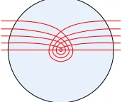
The invisible Eaton lens [8, 11, 14] is a gradient-index (GRIN) lens that looks like

the vacuum from the outside, but has an infinite refractive index at the center. The

refractive index n of the invisible Eaton lens is given by

√

n= 1

nr +

r 1 n2_r2 −1.

One can think the Eaton lens as a Riemannian manifold with the conformally flat

metric n2_g

0 on the unit disk. The metric has a singularity at the center, and the

trajectories of light will be geodesics in that Riemannian manifold.

As can be seen from Figure 1.1, the direction of each light ray when entering

the lens is the same as the direction of the light ray when leaving the lens. Hence

complete circuit inside the Eaton lens,) and thus this Eaton lens is invisible.

Figure 1.1: Trajectories of light in an invisible Eaton lens

Question 1.1.1. Can we have an invisible lens without singularities?

1.2

Scattering rigidity and lens rigidity

Question 1.1.1 is equivalent to asking if flat balls are scattering rigid. Simply put,

a Riemannian manifold M is scattering rigid if M is determined by its scattering

data (see below) up to isometries which leave the boundary fixed.

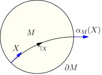
Let π : ΩM → M be the unit tangent bundle of M and ΩxM be the set of

unit tangent vectors at x for any x _∈ M. Let ∂ΩM be the boundary of the unit

tangent bundle of M. In other words, ∂ΩM =S

x∈∂MΩxM. For each x ∈∂M, let νM(x) be the unit normal vector of M pointing inwards at x. Then put∂+ΩxM =

{X _∈ ΩxM : (X, νM(x))gM >0}, ∂0ΩxM = {X ∈ ΩxM : (X, νM(x))gM = 0}, and

∂₋ΩxM = {X ∈ΩxM : (X, νM(x))gM <0}. Also, write ∂+ΩM =

S

x∈∂M∂+ΩxM, ∂0ΩM =Sx∈∂M∂0ΩxM, and ∂−ΩM =Sx∈∂M∂−ΩxM.

For each X _∈ ∂+ΩM, there is a geodesic γX whose initial tangent vector is X.

Let τX :=`(γX), the length ofγX.

If the geodesic γX is of finite length, call its tangent vector at the other end

point αM(X). (See Figure 1.2.) The map αM : ∂+ΩM → ∂ΩM defined above is

called the scattering relation of M. Note that αM(X) will be undefined if γX is of

infinite length.

γX X

αM(X) M

∂M

Figure 1.2: The scattering map αM

Suppose that we have two Riemannian manifolds (M, gM), (N, gN) and an

isom-etry h:∂M _→∂N between their boundaries. Then there is a natural bundle map

ϕ:∂ΩM →∂ΩN defined as

ϕ(aX+bνM(x)) = ah_∗(X) +bνN(h(x)) (1.2.1)

for any unit vector X based at x tangent to ∂M and real numbers a and b such

that a2 _+b2 _{= 1. M and N are said to have the same scattering data rel h if}

ϕ_◦αM =αN_◦ϕ. If we also have `(γX) = `(γϕ(X)), then we say M and N have the

same lens data rel h.

Definition 1.2.1. We say a Riemannian manifoldM is scattering rigid(resp. lens

(resp. lens data) rel h, (where h:∂M _→∂N is an isometry,) we can always extend

h to an isometry from M to N.

We will omit “relh” when his clear from the context or the specific choice ofh

does not matter.

Question 1.2.2 (Equivalent to Question 1.1.1). Are flat balls scattering rigid?

Remark 1.2.3. Theorem 1.3.6 (below) shows that 2-D flat disks are scattering rigid.

Flat balls (of any dimensions) are known (Gromov [10]) to be lens rigid.

1.3

Simple manifolds

Definition 1.3.1. A compact Riemannian manifold with boundary is simple if

1. its boundary is strictly convex,

2. there is a unique minimizing geodesic connecting any pair of points on the

boundary,

3. the manifold has no conjugate points.

Remark 1.3.2. Note that simple manifolds are topological balls.

Conjecture 1.3.3(Michel [15]). Simple Riemannian manifolds are lens (boundary)

rigid.

Theorem 1.3.4 (Pestov–Uhlmann [16]). Simple Riemannian surfaces are lens

Remark 1.3.5. A Riemannian manifold isboundary rigid if its metric is determined

by the distance function between boundary points. The above statements are

origi-nally about boundary rigidity, which is equivalent to lens rigidity when the manifold

is simple. Theorem 1.3.4 confirms the conjecture for surfaces. There are a variety

of results in higher dimensions (Besson–Courtois–Gallot [2], Burago–Ivanov [3, 4],

Croke–Kleiner [7], Michel [15]), but it is still largely open.

Our result extends Theorem 1.3.4 to scattering rigidity.

Theorem 1.3.6. Simple Riemannian surfaces are scattering rigid.

Remark 1.3.7. Simple Riemannian manifolds do not have trapped geodesics and

trapped geodesics often make this type of rigidity problems much harder.

Amaz-ingly, the first (and the only one before this one) known result (Croke [6]) of

scat-tering rigidity is for the flat product metric onS×Dn, which has trapped geodesics.

To get Theorem 1.3.6 from Theorem 1.3.4, it suffices to show that M and N

have the same lens data if they have the same scattering data, assuming that M

is simple. Note that this is not true in general without the assumption that M is

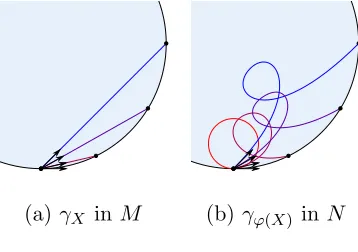
simple. (See Figure 1.3.)

By the first variation of arc length,`(γϕ(X))−`(γX) is equal to a constantL≥0.

If L >0, then γϕ(X) converges to a closed geodesic of length L as X converges to

a vector X0 tangent to the boundary. (See Figure 1.4.) We will call this closed

geodesic γX0.

(a) (b)

Figure 1.3: 1.3b is obtained from 1.3a by removing the upper hemisphere and

identifying antipodal points in the top boundary component. 1.3a and 1.3b have

the same scattering data but different lens data.

(a)γX inM (b)γϕ(X) inN

Figure 1.4: Closed geodesics?

convex as ∂M is convex. However, the convexity of the boundary of a manifold,

being a local property, is not determined by local scattering data as illustrated by

the invisible Eaton lens. The boundary of the invisible Eaton lens is actually totally

geodesic, and we have closed geodesics running along the boundary. The trickiest

part of the proof is to get rid of these closed geodesics using knot theory, (which

1.4

Scheme of the proof

As explained in the previous section, we need to close the gap between lens rigidity

and scattering rigidity, that is, to showL= 0. Recall thatL=`(γϕ(X))−`(γX), the

difference between the lengths of corresponding geodesics inM andN, whereM and

N are two Riemannian manifolds with the same scattering data relh:∂M _→∂N.

In section 2, we will prove thatN is homeomorphic a disk.

Pick any x_∈∂N. IfL >0, then there is a closed geodesicγx of length Lwhich

is tangent to ∂N at x. There are two such closed geodesics for each x, but we can

choose γx properly such that γx moves continuously as xmoves. In this section, we

will assume that γx has multiplicity 1. The actual proof will be more complicated

due to the possibility of higher multiplicities, but the idea of the proof is the same.

The paper will study the isotopy type of the projectivized unit tangent vector

field P _◦ γx˜ : R/Z → PΩN of γx where ˜γx : R/Z → ΩN is the unit tangent

vector field of γx (see (3.1.1) in section 3), PΩN = ΩN/{(x, ξ) ∼ (x,−ξ)} is the

projectivized unit tangent bundle of N, and P : ΩN → PΩN is the corresponding

quotient map.

In section 3 we shall define a family of knot invariants for contractible knots

embedded in PΩN, and then use those invariants to prove Theorem 1.4.1, which is

interesting on its own.

Theorem 1.4.1. P _◦γ˜ is an isotopically non-trivial knot in PΩN for any smooth

Remark 1.4.2. Theorem 1.4.1 is purely knot-theoretical as it involves nether

scat-tering data nor lens data. It is a bit surprising that this simple fact was not known

before even for plane curves. Actually, it would be a completely different story if the

projectivization were drop: Chmutov–Goryunov–Murakami [5] showed that every

knot type in ΩR2 (including the trivial type) is realized by the unit tangent vector

field along an immersed plane curve.

Notice that the union of P ◦γx˜ for all x ∈ ∂N is a torus immersed in PΩN.

We can perturb the immersion to an embedding. Then we can prove that the torus

is compressible by showing that P ◦γx˜ is contractible. (Actually, any embedded

torus in PΩN is compressible.) Next, we can show that the other generator of the

fundamental group of the torus is not contractible in P _◦˜γx. It follows that P _◦γx˜

bounds an embedded disk, which contradicts Theorem 1.4.1. Therefore, there is no

such closed geodesics.

In the actual proof, we shall prove Theorem 1.3.6 in section 4 using a similar

Chapter 2

Topology of

N

Through out the paper (except in section 3), M and N will be two Riemannian

surfaces with the same scattering data rel h : ∂M → ∂N where h is an isometry.

Also, M is assumed to be simple. ϕ : ∂ΩM _→ ∂ΩN is the induced bundle map

defined in (1.2.1). We aim to prove the following result in this section

Proposition 2.0.3. N is homeomorphic to a 2-disk if M is simple.

IfL:=`(γϕ(X))−`(γX) = 0, thenM andN have the same lens data, and hence

N is a 2-disk. Thus we shall assume that L >0 in this section.

Pick a point p0 ∈∂N, and letβ1 : [0,1]→∂N be a constant speed closed curve

of multiplicity 1, starting and ending atp0. There are two such curves corresponding

to different orientations but either one is fine.

Fix an orientation of ∂N and let Y0(x) be the unit vector tangent to ∂N at

as

βx(t) =γY0(x)(Lt),

where γY0(x) is the closed unit speed geodesic tangent to Y0(x) of length L. Write

β2 =βp0.

For any loopβ inN based atp∈N, we will denote by [β]p the based homotopy

class of β. Also, let h : π1(N, p) → H1(N,Z) be the abelianization map which

sends based homotopy classes to corresponding homology classes. We will write

[β] := h([β]p).

Proposition 2.0.4. [β1]p0 = [β2]− 2

p0.

Proof. We shall prove the equivalent statement

[β2]p0 = [β2]

−1

p0 [β1]

−1

p0 . (2.0.1)

Let Y : [0,1]p0 → ∂+ΩN be a smooth curve from Y0(x) to −Y0(x) such that

γYt(τ(Yt)) = β1(t).

DefineH : [0,1]_×[0,1]_→M as

Hs(t) =         

γYs(2τ(Ys)t) if 0≤t≤

1 2,

β1((2−2t)s) if 1₂ ≤t≤1.

Then [H0]p0 = [β2]p0 and [H1]p0 = [β2]− 1

p0 [β1]

−1

p0 , which implies (2.0.1).

Notice that βx are all in the same homology class. Denote bygC the homology

Assume thatgC 6= 0. SinceN is a surface with boundary, it deformation retracts

to a graph, (The deformation is quite simple. Take any cell structure onN. Remove

a 1-cell on the boundary and a 2-cell by deformation retraction if they intersect.

Repeat this process until all 2-cells are removed.) and hence H1(N,Z) = Zn for

some n ∈N. So gC =mg0 for some m > 0 and g0 prime. Then the multiplicity of

βx is at most m since it must divide m. Let m0 be the maximal multiplicity of βx.

Proposition 2.0.5. If gC 6= 0, then H(N,Z) is generated by g0.

Proof. For any g ∈π1(N, p0), letγg : [0,1]→N be the length minimizing

represen-tative of g that is of constant speed Tg. SinceA:=γ−1

g (N\∂N) is open, A= S

A

where _A is a family of disjoint open intervals. For any (a, b)_{∈ A}, sinceγg is length

minimizing, γg|[a,b] has to be a geodesic segment. If a 6= 0, then γ0g(a) has to be tangent to ∂N, orγg will have a corner atγg(a), contradicting the assumption that

γg is length minimizing. According to the scattering data, γ0

g(b) is also tangent to

∂N if γ_g0(a) is tangent to∂N. Henceγg|[a,b] is a closed geodesic tangent to∂N when

a ₆= 0. Similarly,γg_|[a,b] is closed geodesic tangent to∂N whenb 6= 1. Suppose that

a = 0 andb= 1. Ifγ0

g(0) is not tangent to∂N, then γg0(0)/|γg0(0)|=ϕ(X)∈∂+ΩN

for some X ∈ ∂+ΩM, and we have γg0(1)/|γg0(1)| = αM(X). Since M is a sim-ple manifold and X _∈∂+ΩM, γX is a length minimizing geodesic, and thusX and

αM(X) have different base points. It follows thatγg0(0) andγg0(1) also have different base points, contradicting our assumption thatγg is a loop. Therefore, in any case,

that _{|A| ≤} m0Tg/L < ∞. So we can write A = {(a1, b1),(a2, b2), . . . ,(ang, bng)}

where ng =|A| and 0≤a1 < b1 ≤a2 < b2 ≤ · · · ≤ang < bng ≤1.

Since γg_|[ai,bi] is a closed geodesic, [γg|[ai,bi]] = g

ki

0 for some ki > 0. Deleting

all those closed geodesics from γg, we obtain a curve running around ∂N l times

for some l ∈ Z. Its homology class will be [β1]±l = [β2]±2l = g0±2ml. Therefore,

h(g) = g±2m0l+Pngi=1ki

0 . Sinceh is surjective, H1(N,Z) is generated byg0.

Proposition 2.0.6. N is not a M¨obius strip.

Proof. Let π : N1 → N be a double over of N. Then N1 is an annulus with

two boundary components S1 and S2. There are p ∈ S1 and q ∈ S2 such that

d(p, q) = d(S1, S2). Letγ be the shortest curve fromptoq, then γ is perpendicular

to S1 and S2 at tis end points. Let ν be the unit normal vector at p. Since γ is

the shortest curve from p to q, its beginning part must coincide with γν. If the

end point γν(τN1(ν)) is on S1, we can shorten γ by deleting γν. If the end point

γν(τN1(ν)) is on S2, then γ can not be any longer. Thus`(γ) = τN1(ν)

Notice that, for any X _∈ ∂+ΩN1, π◦γX = γπ∗(X). Let Yt be a smooth curve

in ΩpN1 such that Y0 = ν, that Yt ∈ ∂+ΩN1 for t ∈ [0,1) and that Y1 is tangent

to ∂S1. Notice that the end point of π◦γYt =γπ∗(Yt) moves continuously (sinceN

has the same scattering data as the simple surface M), and hence the end point

of γYt moves continuously for t ∈ [0,1). Therefore, γYt connects p and S2 for any

t ∈ [0,1). However, we have `(γ) = τN1(ν) = τN(π∗(ν)) > L, and limt→1`(γYt) =

connecting S1 and S2.

Proof of Proposition 2.0.3. If gC ₆= 0, then H1(N,Z) is generated by g0 by

Propo-sition 2.0.5. Hence H(N,_Z) = _Z, which implies that N is a M¨obius strip, which

contradicts Proposition 2.0.6.

Therefore,gC = 0. It follows thatβ2 is contractible, and henceβ1 is contractible

by Proposition 2.0.4. Since every contractible simple closed curve on a surface

Chapter 3

Knot theory

In this chapter, N will denote a Riemannian surface, with or without boundary,

orientable or not. We assume that there is a Riemannian metric on N just for

convenience and all the results can be stated with only a smooth structure.

3.1

Projectivized unit tangent vector fields

Definition 3.1.1. The unit tangent vector field of a smoothly immersed curve γ

on any Riemannian surface N2 _{(possibly with boundary) is a smoothly immersed}

curve ˜γ in ΩN defined as

˜ γ(t) =

γ(t), γ

0_(t)

|γ0_(t)|

. (3.1.1)

Definition 3.1.2. Let P : ΩN _→ PΩN be the quotient map on the unit

smoothly immersed curve γ in N2_{, P ◦˜γ is called the projectivized unit tangent}

vector field (or the tangent line field) of γ.

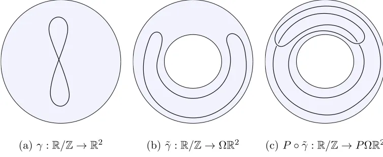
Remark 3.1.3. Chmutov–Goryunov–Murakami [5] showed that every knot type in

ΩR2 is realized by the unit tangent vector field along an immersed closed plane

curve. However, Theorem 1.4.1 shows that it is no longer possible to realize the

trivial knot after the projectivization. Figure 3.1 is an interesting example showing

that the unit tangent vector field of the figure eight curve is an unknot while the

projectivized unit tangent vector field of the figure eight curve is knotted.

(a)γ :R/Z→R2 (b) ˜γ :R/Z→ΩR2 (c) P◦˜γ :R/Z→PΩR2

Figure 3.1: The unit tangent vector field of the figure eight curve is unknotted while

the projectivized unit tangent vector field of the figure eight curve is knotted. Here

the solid tori (Ω_R2 _{and PΩ}

R2) are projected to annuli for illustration.

Proposition 3.1.4. For any smoothly embedded closed curve γ : R/Z → N in

a 2-dimensional manifold N, γ˜ is not contractible in ΩN and hence P _◦γ˜ is not

Proof. If γ is contractible, then γ bounds an embedded disk N1 inN [9, Theorem

1.7].

Let x = ˜γ(0), p = γ(0) and F = π−1_{(p). Denote by [˜γ]}

x the based homotopy

class of ˜γ. As in Figure 3.2, ˜γcorresponds to a vector moving alongγ for a complete

N1

γ(0)

γ(0.25) γ(0.5)

γ(0.75)

(a) ˜γ

N1

(b) Moving base

points towardsp

N1

(c) A generator of

π1(F, x)

Figure 3.2: ˜γ is homotopic to a generator ofπ1(F, x)

circle and being tangent to γ all the time, which is homotopic to a generator of

π1(F, x). Denote the generator of π1(F, x) by g.

Since

F −−−→i ΩN −−−→π N

is a fibration, we have an exact sequence of homotopy groups

π2(N, p) −−−→ π1(F, x)

i∗

−−−→ π1(ΩN, x)

π∗

−−−→ π1(N, p).

If N = S2, then π1(N, p) = 0 and π1(ΩN, p) = π1(RP3,∗) = Z/2Z. Hence

i_∗(π1(F, x)) = Z/2Z. In particular, i∗(e) 6= 0. A similar argument shows that

i_∗(e)₆= 0 when N =RP2. IfN ₆=_S2 _{andN 6=}

RP2, thenπ2(N, p) = 0. Hencei∗ is injective. In particular,

i_∗(e)6= 0.

This completes the proof of Proposition 3.1.4

3.2

Knot invariants

We shall define a family of knot invariants for contractible knots in the projectivized

unit tangent bundle PΩN and use these invariants to prove Theorem 1.4.1.

Let β : R/Z → PΩN be a contractible smooth knot in the projectivized unit

tangent bundle PΩN, whose projection to the surface N2 _{is a smoothly immersed}

curve γ :R/Z→N2 without self-tangencies.

Definition 3.2.1. β has a crossingat(l, l0)∈R/Z×R/Zifl 6=l0 andγ(l) =γ(l0).

Note that a triple crossing will be treated as three independent crossings according

to this definition.

Since β : R/Z → PΩN is contractible, we can lift β to ˆβ : R/Z → ΩN, a

knot embedded in the unit tangent bundle. ( ˆβ(t) is a unit vector at γ(t) but not

necessarily tangent to γ.)

( ˆβ(l),βˆ(l0_{)) and (γ}0_{(l), γ}0_(l0_{)) are of the same orientation. (See Figure 3.3.) A}

crossing will be called negative if it is not positive.

γ

₍

_l

₎

γ

₍

_l

₎

(a) A positive crossing

γ

₍

_l

₎

γ

₍

_l

₎

(b) A negative crossing

Figure 3.3: Each little arrow means a point on ˆβ

.

Lemma 3.2.3. Suppose that γ :_R/_Z→N is a smoothly immersed closed curve on

a surface N without self-tangencies, then all crossings of P ◦γ˜(t) are positive.

Proof. Suppose that P _◦ γ˜ has a crossing at (l, l0_{). Write β = P ◦ γ˜. Then}

( ˆβ(l),βˆ(l0_{)) = (γ}0_{(l), γ}0_(l0_{)), and hence they have the same orientation. Therefore}

the crossing at (l, l0) is positive.

Let X be any topological space. For any two curves α1 : [0,1] → X and

α2 : [0,1] → X such that α1(1) = α2(0), denote by α1∗α2 : [0,1] → X the curve

obtained by gluing α2 toα1. Also, defineR(α1) asR(α1)(t) :=α1(1−t). Ifα1 and

α2 are loops based at p, we have [α1]p[α2]p = [α1 ∗α2]p and [R(α1)]p = [α1]−p1.

topological space X are said to be in the same unoriented free homotopy class if γ1

is homotopic to either γ2 or R(γ2).

When β has a crossing at (l, l0), ˆβ(l) and ˆβ(l0) are two unit vectors with the same base point x = π(β(l)) and they are neither opposite to each other nor the

same (since β is an embedding). Hence there is a unique shortest curve ˆβ(l,l0₎ in

π−1_{(x) connecting ˆβ(l) and ˆβ(l}0_{). Separate ˆβ into two arcs by cutting at ˆβ(l) and}

ˆ

β(l0_{), obtaining two arcs ˆβ}

1 : [0,1]→PΩN and ˆβ2 : [0,1]→PΩN going from ˆβ(l)

to ˆβ(l0_).

Now, letβ₁0 = (P◦βˆ1)∗R(P◦βˆ(l,l0₎), andβ0

2 = (P◦βˆ(l,l0₎)∗R(P◦βˆ₂). Notice that

β0

1 ∗R(β20) is homotopic to β, and hence [β10]p[R(β20)]p = [β10 ∗R(β20)]p = [β]p = e. Hence [β0

1]p = [R(β20)]−p1 = [β20]p. In other words, β10 is homotopic to β20, and hence

β₁0 and β₂0 are in the same unoriented free homotopy class of PΩN.

Definition 3.2.5. The unoriented free homotopy class g(l,l0₎ ofβ0

1 is called the type

of the crossing of β at (l, l0_).

+

Figure 3.4: Smoothing a crossing. Here each little arrow means a point on ˆβ and

Definition 3.2.6. For each nontrivial unoriented free homotopy classg of closed

curves in the projectivized unit tangent bundle PΩN, define

Wg(β) = #_{positive crossings of β of type g_}

−#{negative crossings ofβ of type g}

3.3

W

is a knot invariant.

Theorem 3.3.1. For each non-trivial free homotopy class g, Wg can be extended

to all the contractible knots embedded in PΩN as a knot invariant.

We will show that Wg is a knot invariant by verifying that Wg is unchanged

under Reidemeister moves. A knot will gain or lose a crossing of trivial type after

going through a Reidemeister move of type I. It will gain or lose a pair of crossing

of the same type but opposite signs after going through a Reidemeister move of

type II. Reidemeister moves of type III will not affect crossing. The proof is rather

lengthy because of some technical difficulties.

We will assume that N is compact, and the general case follows automatically

since any manifold is σ-compact.

Definition 3.3.2. According to [1, Theorem 5], there is r >0 such that there is a

unique minimal geodesic segment joining p, q _∈ N if d(p, q)< r. The biggest such

r will be called the injectivity radius of N and we will denote it by inj(N).

π(q) on N. (So dh is a pseudo metric on PΩN.) Notice that p is a projectivized

unit tangent vector at π(p). When dh(p, q) < inj(N), there is a unique shortest

geodesic γ : [0,1] _→ N in N connecting π(p) and π(q). Let X : [0,1] _→ PΩN

be the parallel projectivized vector field along γ such that X(0) = p. Similarly,

let Y : [0,1] → PΩN be the parallel projectivized vector field along γ such that

Y(1) = q. Notice that the angle between X and Y is constant, which is smaller

or equal to π

2. Call this angle dv(p, q). Next, put d

0_{(p, q) = max(d}

h(p, q), dv(p, q)).

Note that dh, dv and d0_{(p, q) are all non-negative and symmetric, but they are not}

metrics.

Definition 3.3.3. For any p, q _∈ PΩN such that dh(p, q) < inj(N) and that

dv(p, q)< π₂, letγ0

p,q : [0,1]→ΩN be the curve that satisfies the following conditions.

1. γ0

p,q(0) =p and γ0p,q(1) =q.

2. π_◦γ is the minimal geodesic connecting π(p) and π(q).

3.

D dtγ

0

p,q

=dv(p, q). (3.3.1)

γ0

p,qwill be called the minimal linear curveconnecting pandq. A curve will be called

linear if it coincides withγ0

p,q for any pair of points p, q on the curve that are close

enough. A curve will be called piecewise linear if it consists of finitely many linear

Proof of Theorem 3.3.1. For any ε < min(inj(N),π

2) and n ≥ 4, we will define

a class of closed piecewise linear knots in PΩN called K(n, ε). A closed knot

β :R/Z→PΩN is in K(n, ε) if and only if the following condition holds:

1. β is contractible.

2. d0_(β(k n), β(

k+1

n ))< ε for k= 0,1, . . . , n−1.

3. β(k+_nt) =γ0

β(k n),β(

k+1 n )

(t) for t∈[0,1] andk = 0,1, . . . , n−1.

In other words, the “distance” (dh and dv) between any two adjacent vertices p

and q is at most ε and the edge between them is γp,q0 . K(n, ε) is an open subset of

(PΩN)n_{, and thus of dimension 3n.}

Let β _{∈ K}(n, ε) be a piecewise smoothcontractible knot with vertices _{xk =

β(k_n)} and edges {ek = γx0k,xk+1}. Its projection π◦β is said to have a singularity

at the vertex π(xi) if π(xi) is on the π◦ej for some i /∈ {j, j+ 1}.

Let_Kk(n, ε) be the set of knots in K(n, ε) whose projections onN have at most

k singularities. Also, let K0

k(n, ε) = Kk(n, ε)− Kk−1(n, ε), knots with exactly k

singularities. Then K0(n, ε) is a open submanifold of K(n, ε), and K10(n, ε) is a

submanifold of _K(n, ε) of co-dimension 1.

Notice that the Wg(β) can be defined for β ∈ K0(n, ε) as before without any

modifications. Consider a continuous family of knots βt ∈ K0(n, ε). As t varies,

crossings of βt also moves continuously with their types unchanged. Therefore, Wg

Next, we extend Wg toK1(n, ε). The old definition can not be adapted directly

since there might singularities. Pick any β0, β1 ∈ K0(n, ε) such that β0, β1 are in

the same component of _K1(n, ε). We aim to show thatWg(β0) =Wg(β1), and then

we can extend Wg toK1(n, ε) by making it constant on each component. Note that

Wg will remain the same on K0(n, ε).

Pick a smooth path H : [0,1] _{→ K}1(n, ε) from β0 to β1. Perturbing H if

necessary, we may assume that H intersects _K0

1(n, ε) transversely a finite number

of times. Let x0(t),x1(t), . . . ,xn(t) =x0(t) be then vertices ofH(t).

As long as H(t) stays in _K0(n, ε), each crossing will just be moving without

changing its type. When H(t) passes through _K0

1(n, ε), there are three

possibili-ties corresponding to three types of singularipossibili-ties for knots in K0

1(n, ε) listed below.

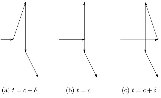
Suppose H(c) _{∈ K}0

1(n, ε) and H(t) ∈ K/ 10(n, ε) for t ∈ (c−δ, c)

S

(c, c+δ). Then

π_◦H(c) has a singularity atπ(xi(c)) which is on π◦ej wherexi(c) is thei-th vertex

of H(c) and ej(c) is j-th edge of H(c) (connecting xj(c) and xj+1(c)).

1. If π_◦ei(c) or π_◦ei₋1(c) is tangent to π◦ej(c), then the singularity is called

a cusp. This happens when i = j ₋1 or i = j + 2. In this case, H(c+δ)

has one more or one less crossing than H(c−δ) has. We will show that the

crossing involved is of the trivial type, (i.e.,g = 0,) and henceWg(H(c₋δ)) =

Wg(H(c+δ)) for any non-trivial unoriented homotopy classg of closed curves

immersed in PΩN.

(a) t=c₋δ (b) t=c (c)t=c+δ

Figure 3.5: 3.5c has one more crossing of the trivial type compared to 3.5a. This

corresponds to a Reidemeister move of type I.

more crossing at (l(t), l0(t)) than H(t0) has when c −δ ≤ t0 < c < t ≤

c+ δ. (See Figure 3.5.) For any t _∈ (c, c+δ], swapping l(t) and l0_{(t) if}

necessary, we may assume that l(t)∈ (i−_n1,_ni) and l0(t)∈ (i+1_n ,i+2_n ). Lift H : [0,1] → K(n, ε) to ˆH : [0,1] → (R/Z → ΩN). Since H(t) is an embedding,

H(t)(l(t))=₆ H(t)(l0_{(t)), and hence ˆH(t)(l(t)) and ˆH(t)(l}0_{(t)) are not opposite}

vectors. It follows that there is a unique minimal geodesic ˆα(t) : [0,1] →

π−1_{(x) connecting ˆH(t)(l(t)) and ˆH(t)(l}0_{(t)). Let α(t) = P ◦αˆ(t) and glue}

α(t) to H(t)_|[l(t),l0_(t)], obtaining a closed curve C(t). Then the type of the

crossing of H(t) at (l(t), l0(t)) is the unoriented homotopy class of C(t). It remains to show that C(t) is contractible.

Let l(c) = limt→c+l(t) and l0(c) = limt→c+l0(t), then C(c) can be defined as

before, which is homotopic to C(t) fort _∈(c, c+δ). We shall show that C(c)

Reparametrize C(c) as ¯β :R/Z→PΩN such that ¯β(0) =H(c)(l(c)), ¯β(1₃) =

xi+1(c), ¯β(2₃) = H(c)(l0(c)) and π( ¯β(1₃(1 + s))) = π( ¯β(1₃(1− s))) for any

s _∈[0,1]. To be precise, define ¯β as

¯ β(t) =

                  

H(c)(i+3t

n ) if t∈[0,

1 3],

H(c)(i+1

n + (3t−1)(l0(c)− i+1

n )) if t∈[

1 3,

2 3],

α(3₋3t) if t_∈[2

3,1].

Consider the homotopy G: [0,1]→(R/Z→PΩN) defined as

G(s)(t) =                    ¯

β(t) if 0_≤t_≤ 1

3(1−s),

T( ¯β(t), π( ¯β(1

3(1−s)))) if 1

3(1−s)≤t≤ 1

3(1 +s),

¯

β(t) if 1

3(1 +s)≤t ≤1,

whereT( ¯β(t), π( ¯β(₃1(1₋s)))) is a projectivized unit tangent vector atπ( ¯β(1₃(1₋

s))) obtained by transporting ¯β(t) parallelly along π_◦ej(c). Notice thatG(1)

is a closed curve in Ωπ(xi)N, where Ωπ(xi)N is a circle of length 2π, (using the

Sasakian metric). We are going to show that G(1) is contractible by showing

that `(G(1))<2π. For any piecewise smooth curve γ : [a, b]_→PΩN, define

its vertical length as

`v(γ) := Z b a D dtγ(t)

dt, where D

dt is the covariant derivative. Loosely speaking, `v(γ) measure the

is constant as s goes from 0 to 1. Notice that ¯β has three edges. The edge

from ¯β(0) to ¯β(1₃) and the edge from ¯β(1₃) to ¯β(2₃) both have vertical lengths

at most ε (by (3.3.1)), and the vertical length of the edge from ¯β(2₃) to ¯β(0)

(which is reparametrized α) is at most π. Since ε < π

2, `v( ¯β)< π+ 2ε <2π,

and hence `(G(1)) =`v(G(1)) = `v(G(0)) = `v( ¯β)<2π. It follows that G(1)

is contractible, and hence C(t) is contractible for anyt _∈[c, c+δ].

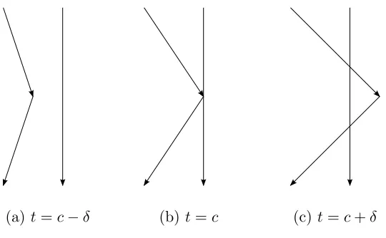
2. If π_◦ei(c) and π◦ei−1(c) are not tangent to π◦ej(c), and if π◦ei(c) and π ◦ei₋1(c) are on the same side of π ◦ej(c), then the singularity is called a

self-tangency. In this case, H(c+δ) has two more or two less crossings than

H(c₋δ) has. We can show that the two crossings involved are of the same

type g but opposite signs, and hence Wg(H(c+δ)) =Wg(H(c−δ)).

Without loss of of generality, assume that H(t) has two more crossing at

(l1(t), l01(t)) and (l2(t), l20(t)) than H(t0) has when c−δ ≤t0 < c < t ≤c+δ.

(See Figure 3.6.) Let l1(c) = limt→c+l1(t) and define l01(c), l2(c) and l02(c)

similarly. Switching l2 and l02 if necessary, we may assume that l1(c) = l2(c)

and l₁0(c) = l0₂(c). Also, either H(l1(c)) =xi or H(l10(c)) =xi. Without loss

of generality, we assume that H(l1(c)) = xi. Lift H : [0,1] → K(n, ε) to

ˆ

H : [0,1]→(R/Z→ΩN), and denote the vertices of ˆH(t) by ˆxk(t) and edges

by ˆek(t).

For anyt ∈(c, c+δ], we can separate ˆH(t) into two arcs by cutting at ˆH(l1(t))

and ˆH(l0

(a) t=c₋δ (b) t=c (c)t=c+δ

Figure 3.6: 3.6c has two more crossing of the same type but opposite signs compared

to 3.6a. This corresponds to a Reidemeister move of type II.

it to ˆH(l1(t),l01(t)), obtaining a closed curve C1(t). We can also separate ˆH(t)

into two arcs by cutting at ˆH(l2(t)) and ˆH(l20(t)). Pick the arc which does not

contain the lift of the vertex xi and glue it to ˆH(l2(t),l02(t)), obtaining a closed

curve C2(t). Next, define C1(c) and C2(c) by taking limits. It is then clear

that P ◦C1(t) andP ◦C2(t) are in the same unoriented homotopy class since

C1(c) = C2(c). Hence the two crossings at (l1(t), l01(t)) and (l2(t), l20(t)) are of

the same type.

Finally, it remains to show that the two crossings have opposite signs. Without

loss of generality, assume that the crossing at (l1(t), l01(t)) is positive. In other

words, ( ˆH(l1(t)),Hˆ(l01(t))) and ((π◦H)0(l1(t)),(π◦H)0(l10(t))) have the same

orientation. It follows that ( ˆH(l1(c)),Hˆ(l10(c))) and (limt→c+(π◦H)0(l1(t)),(π◦

H)0(l₁0(c))) have the same orientation. Since π ◦ ei(c) and π ◦ ei₋1(c) are

(limt→c+(π◦H)0(l2(t)),(π◦H)0(l02(c))) have the opposite orientation. Since

( ˆH(l1(c)),Hˆ(l10(c))) and ( ˆH(l2(c)),Hˆ(l20(c))) are the same, ( ˆH(l2(c)),Hˆ(l20(c)))

and (limt→c+(π◦H)0(l2(t)),(π◦H)0(l20(c))) have the opposite orientation, and

thus the crossing at (l2(t), l20(t)) is negative.

3. If π◦ei and π◦ei−1 are not tangent to π◦ej, and if π◦ei and π◦ei−1 are

on different sides of π _◦ej, then the singularity is called a transverse

self-intersection. In this case, all crossings moves continuously as tgoes fromc₋δ

toc+δ, although one crossing will be also a singularity att=c. The type and

the sign of that crossing will be unchanged, which follows from an argument

very similar to the one used for the previous case.

In any case, we have Wg(H(c−δ)) = Wg(H(c+δ)) for any non-trivial type g. It

follows that Wg(β0) = Wg(H(0)) = Wg(H(1)) = Wg(β1), and thus we may extend

Wg to _K1(n, ε) by making it constant on each component.

Next, we will extent Wg to the whole K(n, ε). Pick any β0, β1 ∈ K1(n, ε) such

that β0, β1 are in the same component of K(n, ε). We aim to show that Wg(β0) =

Wg(β1), and then we can extend Wg to K(n, ε) by making it constant on each

component.

The manifold _K(n, ε) has a natural stratified structure as follows. For any

γ _{∈ K}(n, ε), pick any neighborhood U of γ. If γ has k singularities, then let Uγ be

the component of UT

K0

k(n, ε) containing γ, which is a submanifold embedded in

x1

x2 x3

x4

x5

x6 x7

x8

x9

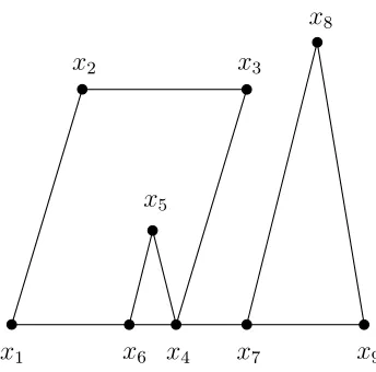
Figure 3.7: This is the projection of a knot β ∈ X3 to N. Notice that x4 is on

the edge from x9 to x1 and also the edge from x6 to x7. Hence, there are two

singularities involving x4. There are also two singularities involvingx6 andx7, and

thus β ∈ K0

4(9, ε). This counterexample shows that Xm = K03n−m(n, ε) is not true in general when m is big.

space whose m-dimensional stratum is Xm. We obviously haveX3n =K0(n, ε) and

X3n−1 = K01(n, ε). (Note that Xm = K03n−m(n, ε) is not true when m is big since the singularities are not necessarily independent. See Figure ??.) Pick a smooth

path H : [0,1] → K1(n, ε) from β0 to β1. Perturbing H if necessary, we may

assume that H intersects each stratum Xm transversely. In other words, H does

not intersect Xm at all if m < 3n−1. Hence H is actually a path in K1(n, ε),

and thus Wg(β0) =Wg(β1). Therefore, we can extend Wg to K(n, ε) by making it

constant on each component.

Now, we can extend Wg to a knot invariant for all contractible knots embedded

contractible knot β, we can approximate β by a piecewise linear knot β0 _{that is}

homotopic to β. Then we set Wg(β) = Wg(β0). Wg is well-defined according to Lemma A.0.9.

Now, we are ready to prove Theorem 1.4.1.

Proof of Theorem 1.4.1. Letβ =P◦γ˜be the projectivized unit tangent vector field

of γ.

If β is not contractible, then β is a non-trivial knot. Assume that β is

con-tractible. We are going to show that Wg(β)>0 for some g, whileWg(Unknot) = 0

for any g.

Assume thatγ has no self-intersections. Then β is not contractible by

Proposi-tion 3.1.4. So γ has at least one self-intersection.

We will start at any point on γ and trace along γ until hitting the trace. To be

precise, letq = max_{t:γ_|[0,t] has no self-intersection}. Then there isp∈[0, q) such

that γ(p) = γ(q) and β has a crossing at (p, q). By Lemma 3.2.3, the crossing of

β at (p, q) is positive. Separate ˆβ into two arcs by cutting at ˆβ(p) and ˆβ(q). Then

ˆ

β_|[p,q]will be one of these two arcs. Glue ˆβ|[p,q]to ˆβ(p,q), obtaining a closed curve ˆβ0.

We can gradually widen the angle of γ|[p,q] at the corner until it becomes a simple

smooth closed curve, and ˆβ0 _{will converge to the unit tangent vector field along that}

simple smooth closed curved. By Proposition 3.1.4, ˆβ0 _{is not contractible in ΩN.}

Actually, a stronger (but more technical) result can be proved with exactly the

same proof.

Theorem 3.3.4. Suppose that γ1 : [0,1]→N is smoothly immersed curve without

self-tangencies and that β2 : [0,1]→PΩN is a smoothly embedded curve connecting

the end points of β1 :=P◦˜γ. Glueβ2 toβ1, obtaining a closed curve β in PΩN. If

γ1 has at least one self-intersection, γ1 and π◦β2 have no intersections and π◦β2

has no self-intersections, then β is isotopically non-trivial.

Proof. Just let

β =

    

   

β1(2t) if t∈[0,1₂],

β2(2−2t) ift∈[1₂,1].

and γ = π _◦β. Let q = max_{t : γ_|[0,t] has no self-intersection}. Then there is

p∈[0, q) such that γ(p) = γ(q) and β has a crossing at (p, q).

Note that q < 1

2 because γ1 has at least one self-intersection. The rest of the

Chapter 4

Closed geodesics tangent to the

boundary

In this section, M and N will be two Riemannian surfaces with the same scattering

data rel h : ∂M _→∂N where h is an isometry. Also, M is assumed to be simple.

ϕ:∂ΩM →∂ΩN is the induced bundle map defined in (1.2.1). In this section, we

shall prove Theorem 1.3.6 by studying closed geodesics tangent to the boundary.

Recall that L = τN(ϕ(X))−τM(X) ≥ 0 is a constant. We need to show that

L= 0.

For any Y _∈ ∂0ΩN, Recall that γY is the limit of geodesic segments γX as

X _→Y where X _∈∂+ΩN. γY is a closed geodesic of length L.

Proposition 4.0.5. If L > 0, then P ◦γY˜ is contractible in PΩN for any Y ∈

Proof. Pick p_∈∂ΩN. LetY _∈∂0ΩpN be one of the two unit vector atpwhich are

tangent to ∂N. Put

Ys = cos(πs)Y + sin(πs)ν(x),

for each s_∈[0,1].

Now define a continuous family of loops H : [0,1]×R/Z→ΩN as

Hs(t) =                    γ0

Ys(3τ(Ys)t) if 0≤t≤

1 3,

αN(Y(2−3t)s) if 1₃ ≤t≤ 2₃,

Y(3t−2)s if 2₃ ≤t≤1.

We shall show that H1|[1

3,1] is contractible. Since N is a disk, there is a

diffeo-morphism ψ :N → {(x, y)∈ R2 : x2 +y2 ≤ 1}. For any X ∈ ΩN and x ∈ N, let

ξ(x, X) be the unit vector based at x such that ψ_∗(ξ(x, X)) and ψ_∗(X) have the same directions as two vectors in _R2_.

Since N is a disk, ∂N is homotopic the constant curve at p. So there is a

homotopy q: [0,1]_×[0,1]_→ N such that q(1,_·) =p and thatq(0, t) =π(αN(Yt)).

Next, define a continuous family of loops G: [0,1]_×R/_Z→ΩN as

Gs(t) =         

ξ(q(s,2t), αM(Y2t)) if 0≤t ≤ 1₂,

Y2−2t if 1₂ ≤t ≤1.

Let At be the angle that r1(t) :=ξ(p, αM(Y¯_t)) rotates by as ¯t goes from 0 to t. We

by as ¯t goes from 0 to t. Notice that ψ(q(0,¯t)) goes around the unit circle in R2

for a full circle as t goes from 0 to 1. Hence B1 = 2π. Let Ct be the signed angle

between r1 and r2. Since r1(0) and r2(0) have the same direction, Ct = Bt−At.

For any t_∈(0,1), αM(Y¯t) is not tangent to∂N, and hence Ct ∈[0, π] fort∈[0,1].

Since r1(1) and r2(1) have opposite directions,C1 =π, which implies that A1 =π.

Therefore, ξ(p, αM(Yt)) rotates counterclockwise by π as t goes from 0 to 1. On

the other hand, the Y2−2t rotate by π clockwise ast goes from 1₂ to 1. Hence G1 is

contractible. It follows that G0 is contractible, and thusH1|[1

3,1] is contractible.

SinceH0|[1

3,1] is constant andH0|[0, 1

3] coincides with ˜γY, H0 is homotopic to ˜γY.

Since H1|[1

3,1] is contractible and H1|[0, 1

3] coincides with ˜γ−Y, H1 is homotopic to

˜

γ₋Y. Therefore, ˜γY is homotopic to ˜γ−Y.

If we rotate each vector counterclockwise byπ, then ˜γ₋Y becomesR(˜γY). Hence ˜

γY is homotopic to R(˜γY). It follows that [˜γY] = [R(˜γY)] = −[˜γY], where [α]

means the homology class of α. Since N is a disk, ΩN is a solid torus, and hence

H1(ΩN,Z) = Z. Thus [˜γY] = 0, that is, ˜γY is contractible. Hence P ◦ γY˜ is

contractible in PΩN.

Fix an orientation of ∂N and let X0(x) be the unit vector tangent to ∂N at

x_∈∂N such thatX0(x) and∂N have the same orientation. Leth1 :R/Z→∂N be

an orientation preserving diffeomorphism. Pick ε > 0 small and let T :∂N _→∂N

be a diffeomorphism defined as

and let X1(x) ∈ ∂+ΩxN be the vector which is tangent to the geodesic from x to

T(x). Finally, put X2(x) = α(X1(T−1(x))). When T−1(x), x and T(x) are close,

bothX1(x) andX2(x) are close toX0(x), so we may assume that the angle between

X1(x) and X2(x) is smaller than π by pickingε small enough. See Figure 4.1.

N

X0(x)

X1(x)

X2(x)

X1(T−1(x))

T(x)

x T−1_(x)

Figure 4.1

Now X1(x) and X2(x) separate the circle ΩxN into two segments. Let A(x)

be the segment containing X0(x) (which is the shorter segment). Then A =

S

x∈∂NA(x) is an annulus with boundariesX1(∂N) andX2(∂N). We have a natural diffeomorphism u:R/Z×[0,1]→A whereu(s, t) is the unique vector in ∂Ωh1(s)N

such that

t= The angle between u(x, t) andX1(h1(s)) The angle betweenX1(h1(s)) and X2(h1(s))

.

In particular, we have u(s,0) = X1(h1(s)) andu(s,1) =X2(h1(s)).

from X1(x) to α(X1(x)) defined as

ηh1(s)(t) = u(s+εt, t).

See Figure 4.2.

N

ηx(0)

ηx(1)

T(x)

x

Figure 4.2: Values of ηx from 0 to 1

f(x,0) =f(x,1)

f(x,1−ε)

N

x

T(x)

Figure 4.3: Values of f(x,_·) from 0 to 1

Define

as

f(x, t) =     

   

P γX˜ 1(x)(

t

1−ε)

if 0_≤t_≤1₋ε,

P ηx(1−t ε )

if 1₋ε_≤t_≤1.

See Figure 4.3.

Proposition 4.0.6. f :∂N ×R/Z→PΩN is an embedding.

Proof. Suppose that f(x, t) = f(x0_{, t}0_{). If 0 < t < 1−ε, then π(f(x, t)) is not}

on the boundary, so π(f(x0_{, t}0_{)) is also not on the boundary, which implies that}

0< t0 <1−ε. However, π◦f(x,·)|(0,1−ε) and π◦f(x0,·)|(0,1−ε) are geodesics in N,

so they always intersect transversely, and thus f(x, t) and f(x0_{, t}0_{) are equal if and}

only if (x, t) = (x0_{, t}0_{). If 1−ε≤t≤1, then 1−ε≤t}0 _{≤1. Now f(x, t) =P(η}

x(t))

and f(x0, t0) = P(ηx0(t0)), where P : A → PΩN is injective because the angle between X1(x) and X2(x) is smaller than π. Hence f(x, t) = f(x0, t0) if and only

if ηx(t) = ηx0(t), which, by our definition of η, is equivalent to (x, t) = (x0, t0). Therefore,f is an embedding of the torusR/Z×∂N into the solid torusPΩN.

Proposition 4.0.7. f(x,_·) is contractible in PΩN.

Proof. We shall show thatf(x,_·) is homotopic toP_◦˜γX0(x). Asε→0,T converges

to the identity map,X1andX2 converge toX0, andf(x,₁₋t_ε) converges toP(˜γX0(t))

for t _∈[0,1₋ε]. Thus f(x,_·) is homotopic to P _◦˜γX0(x).

Proof. Define β1 :R/Z→∂N ×R/Z as

β1(t) = (h1(t),0),

and define β2 :R/Z→∂N ×R/Zas

β2(t) = (h1(0), t).

Let p=β1(0), then

π1(∂N ×R/Z, p) = {[β1]kp[β2]lp :k, l∈Z} 'Z2.

Let

f_∗ :π1(∂N ×R/Z, p)→π1(PΩN, f(p))

be the induced homomorphism between fundamental groups. Sinceπ1(PΩN, f(p)) =

Z, f∗ is not injective. Since [12, Corollary 3.3] a two-sided surface f is

incompress-ible if and only if f_∗ is injective, the torus f(∂N ×R/Z) has a compressing disk embedded in PΩN.

As ε _→ 0, f _◦ β1 converges to the projectivized unit tangent vector field

along ∂N, so f_∗([β1]p) 6= 0 by Proposition 3.1.4. Since f(h1(0),·) is homotopic

to γX0(h1(0)), both of them are contractible in PΩN by Proposition 4.0.5. Since

π1(PΩN, f(p)) =Z, there is no difference between free homotopy and based

homo-topy, hence f_∗([β2]p) = 0.

Now, let B be a compressing disk of the torus f(∂N _×R/Z), then ∂B is a

homotopic to f _◦β2 on f(R/Z×S). Any two simple closed essential curves on a

surface are isotopic to each other if and only if they are freely homotopic to each

other [9]. Therefore, ∂B is isotopic to f _◦β2 =f(h1(0),·) on f(R/Z×S)⊂PΩN.

Since ∂B bounds a disk B inPΩN, ∂B is isotopically trivial, and so is f(h1(0),·)

in PΩN. This completes the proof of Proposition 4.0.8

Notice (see below) that Proposition 4.0.8 contradicts Theorem 3.3.4 whenL >0,

which proves Theorem 1.3.6.

Proof of Theorem 1.3.6. Suppose that L > 0. Pick any x ∈ ∂M. Let γ1 = γX1(x)

and β2 =P ◦ηx.

If γ1 has no self-intersections, then γX0(x), the limit of γ1 as ε → 0, also has

no self-intersections. By Proposition 3.1.4, P ◦˜γX0(x) is not contractible in PΩN1,

which contradicts Proposition 4.0.5. Therefore, γ1 has at least one self-intersection.

Let β1 =P ◦˜γ1 Notice that γ1 and P ◦β2 have no intersections except at end

points and thatf(x,·) is the closed curve obtained by gluingβ1andβ2. By Theorem

3.3.4,f(x,_·) is isotopically non-trivial inPΩN1, which contradicts Proposition 4.0.8.

Appendix A

Approximating smooth knots by

piecewise linear knots

The goal of this section is to prove the following lemma, which allows us to

approx-imate knot isotopies using piecewise-linear knot isotopies.

Lemma A.0.9. Suppose that there is a continuous knot isotopyG: [0,1]×R/Z→

PΩN. Then there is continuous family of knot isotopiesH : [0,1]_×[0,1]_×R/Z→

PΩN such that H(0,·,·) = G, that H(l, s,·) is a knot embedded in PΩN for each

(l, s)∈[0,1]×[0,1], and that H(1, s,·)is a piecewise linear knot for each s∈[0,1].

The following proposition and its corollaries will be our main tool used in this

section.

Riemannian manifold. Suppose that G : K _×[a, b] _→ M is smooth and that each

G(s,·) is a smooth curve whose speed is never 0. For any ε > 0, there is δ > 0

such that the angles between G(s,_·)_|[t1,t2] and the minimal geodesic connecting its

end points are smaller than ε whenever _|t1−t2|< δ.

Proof. Pick any ε >0. There is ε1 >0 such that|θ|< ε if |cos(θ)−1|< ε1 and if

|θ_{| ≤}π.

DefineL:K_×[a, b]_×[a, b]_→R as

L(s, t1, t2) =

        

`(G(s,·)|[t1,t2]) ift2 ≥t1,

−L(s, t1, t2) if t2 < t1,

where `(G(s,_·)_|[t1,t2]) is the length of G(s,·)|[t1,t2]. Similarly, defineD:K×[a, b]×

[a, b]_→Ras

D(s, t1, t2) =

        

d(G(s, t1), G(s, t2)) if t2 ≥t1,

−D(s, t1, t2) if t2 < t1.

For any fixed s, we have

L(s, t1, t2)−D(s, t1, t2) =o((t2−t1)2) (A.0.1)

as t2 →t1. Put

Q(s, t1, t2) =

∂

∂t2D(s, t1, t2)

∂

∂t2L(s, t1, t2)

.

We shall show theQis continuous nearK_×∆[a, b] where ∆[a, b] is the diagonal

of [a, b]×[a, b]. Since G is continuous and K is compact, there is δ1 > 0 such

that d(G(s, t1), G(s, t2)) < inj(M) if |t1 −t2| < δ1. Since the squared distance

function is smooth within the injectivity radius, D2 _{is smooth on K ×V}

δ1 where

Vδ1 = {(t1, t2) ∈ [a, b]×[a, b] :|t1−t2| < δ1} and hence

∂

∂t2D is continuous. Also,

∂

∂t2L is obviously continuous on K×[a, b]×[a, b] (sinceL(s, t1,·) is just the signed

arc length). Therefore, Qis continuous on K_×Vδ1. Since Qis continuous andK is

compact, there is δ∈(0, δ1) such that |Q(s, t1, t2)−Q(s, t1, t1)|< ε1 if |t1−t2|< δ,

that is, _|Q₋1_|< ε1 on K×Vδ.

For any (s, t1, t2)∈K×Vδ\∆[a, b], letθ(s, t1, t2) be the angle betweenG(s,·)|[t1,t2]

and the minimal geodesic connecting its end points at the endpoint G(s, t2). By

the first variation of arc length,

cosθ(s, t1, t2) =

∂

∂t2D(s, t1, t2)

∂

∂t2L(s, t1, t2)

=Q(s, t1, t2).

Hence θ < εonK×Vδ. Therefore the angles betweenG(s,·)|[t1,t2]and the minimal

geodesic connecting its end points are smaller than ε whenever _|t1−t2|< δ.

For any compact Riemannian surfaceN, we can apply the above proposition to

unit-speed linear curves of length _≤1 in PΩN (which has the Sasakian metric on

it), which is a compact family of curves in PΩN. For any p, q _∈ PΩN such that

d(p, q) < inj(PΩN) and that dh(p, q) < inj(N), let γp,q be the minimal geodesic

connecting pandq. Recall thatγ0

Corollary A.0.11. Assume that N is a compact Riemannian manifold. For any

ε > 0, there is δ > 0 such that the angles between γp,q and γ0

p,q are smaller than ε

for any p, q _∈PΩN such that 0< d(p, q)< δ.

Suppose that p, q, r _∈ PΩN are close enough that there are minimal linear

curves γ0

p,q, γq,r0 and γp,r0 . Denote by A(p, q, r) the sum of the three angles between

γ0

p,q, γq,r0 and γp,r0 . Since the sum of the inner angles of small geodesic triangles are

close to π, Corollary A.0.11 implies that A(p, q, r) is also close to π when p, q and

r are close enough.

Corollary A.0.12. Assume that N is a compact Riemannian manifold. For any

ε > 0, there is δ > 0 such that _|A(p, q, r)−π|< ε for any p, q, r ∈PΩN such that

d(p, q), d(p, r), d(q, r)_∈(0, δ).

The following result follows from Proposition A.0.10 and Corollary A.0.11.

Corollary A.0.13. Assume that K is a compact smooth manifold and N is a

compact Riemannian manifold. Suppose that G:K_×[a, b]_→PΩN is smooth and

that each G(s,·) is a smooth curve whose speed is never 0. For any ε >0, there is

δ >0 such that the angles between G(s,_·)_|[t1,t2] and γ 0

G(s,t1),G(s,t2) are smaller than ε

whenever _|t1−t2|< δ.

Proof of Lemma A.0.9. We shall assume that G is smooth since it is standard to

approximate continuous isotopies by smooth isotopies.

Putε = 0.1. By Corollary A.0.13, there is δ1 >0 such that the angles between

G(s,_·)_|[t1,t2]andγ 0

A.0.12 there is ε0 >0 such that

|A(p, q, r)−π|< ε (A.0.2)

for any p, q, r ∈ PΩN such that d(p, q), d(p, r), d(q, r)∈ (0, ε0). Also, by corollary

A.0.11, there is ε1 ∈ (0, ε0) such that the angles between γp,q0 and γp,q are smaller

than ε for any p, q ∈PΩN such that 0 < d(p, q)< ε1. SinceG is continuous, there

is δ2 ∈(0, δ1) such that d(G(s, t1), G(s, t2))< ε1 if d(t1, t2)< δ2.

For each (s, t) _∈ [0,1]_×R/Z, let I(t) = R/Z\(t−δ2, t+δ2), then D(s, t) :=

d(G(s, t), G(s, I(t))) > 0. Let ε2 = min(ε1,inf(s,t)∈[0,1]×R/ZD(s, t)), then ε2 > 0. Since G is continuous, there is δ ∈ (0, δ2) such that d(G(s, t1), G(s, t2)) < 1₂ε2 if

d(t1, t2)< δ.

Pick n∈N such that nδ >1. Define H : [0,1]×[0,1]×R/Z→PΩN as

H(l, s,k+t

n ) =

         γ0

G(s,k n),G(s,

k+l n )

(t_l) if 0 ≤t < l

G(s,k+_nt) if l ≤t ≤1

where k _{∈ Z}/n_Z, and t _∈ [0,1]. It is obvious that H(0,_·,_·) = G and H(1,_·,_·) is

an isotopy of piecewise linear knots. We shall show that each H(l, s,·) is a knot

embedded in PΩN.

Suppose thatH(l, s,_·) has a self-intersection, that is,H(l, s,k1+t1

n ) =H(l, s, k2+t2

n )

for some ki ∈Z/nZand ti ∈[0,1) such that k1 6=k2 or t1 6=t2.

Since G(s,_·) is an embedding, we have either t1 < l or t2 < l. Without loss of

γ0

G(s,k1 n),G(s,

k₁₊l n )

is in Nε₂ 2 (G(s,

k1

n)), the ball of radius ε2

2 centered at G(s,

k1

n). Put

p = G(s,k1

n) and q = G(s, k1+l

n ). Since d( k1

n, k1+l

n ) < δ <

1

3δ2, d(p, q) < ε1. Define

Q: [0,1]_→R as

Q(t) = ∂ ∂td(p, γ

0

p,q(t)) ∂

∂t`(γp,q0 |[0,t])

By the first variation of arc length, Q(t) = cosθ(t) where θ(t) is the angle between

γ0

p,q|[0,t]and the minimal geodesic connecting their end points at the end pointγp,q0 (t).

Since d(p, q)< 1

2ε2 < ε1,θ(t)< ε= 0.01, and henceQ(1)>0. IfQ(t) = 0 for some

t ∈ [0,1), then let t0 = sup{t ∈ [0,1) : Q(t) = 0}. Then we have Q(t0) = 0 and

Q(t)>0 fort ∈(t0,1]. Since

d(p, γ_p,q0 (t0)) =d(p, q)−

Z 1

t0

∂ ∂td(p, γ

0

p,q(t))dt

=d(p, q)−

Z 1

t0

∂

∂t`(γp,q|[0,t])

Q(t) dt

< d(p, q)

< ε1,

θ(t0) < ε, and hence Q(t0) > 0, which contradict our assumption that Q(t0) = 0.

So Q(t)> 0 for any t _∈[0,1], which implies that d(p, γ0

p,q(t)) is strictly increasing.

Hence d(p, γ0

p,q(t)) ≤ d(p, q) < ε22 for all t ∈ [0,1), that is, γ 0

G(s,k1+l n ),G(s,

k₁ n)

is in

Nε2

2 (p). It also follows thatγ 0

G(s,k1+l n ),G(s,

k₁ n)

has no self-intersections, and thusk1 6=

k2.

Assume that d(k1

n, k2

n) ≥ δ2. Then G(s, k2

n) ∈/ Nε2(G(s,

k1

n)). Hence we have

Nε2 2 (G(s,

k1

n)) T

Nε2 2 (G(s,

k2

n)) = ∅. When t2 ≤ l, H(l, s, t4) is on γ_G0_(s,k₂ n),G(s,

k₂₊l n )

which is contained in Nε₂ 2 (G(s,

k2

n)), and hence H(l, s, t4) ∈ Nε22(G(s,

k2

n)).

How-ever, for the same reason, H(l, s, t3) ∈ Nε2 2 (G(s,

k1

n)), and hence H(l, s, t3) 6=

H(l, s, t4), which contradicts our assumption. When t2 ≥ l, H(l, s, t4) = G(s, t4).

Since d(k2

n, t4) = t n <

1

n < δ, d(G(s, k2

n), G(s, t4)) < ε2

2 , and hence H(l, s, t4) ∈

Nε2 2 (G(s,

k2

n)). Again, H(l, s, t3) 6= H(l, s, t4), which contradicts our assumption.

Therefore,d(k1

n, k2

n)< δ2. We shall assume that k2

n ∈(

k1

n, k1

n+δ2), and the other case

(k1

n ∈(

k2

n, k2

n+δ2)) can be addressed similarly. Then we haved(H(l, s, k1+l

n ), H(l, s, k2

n))<

ε2.

We shall show that d(G(s,k2

n), H(l, s, t4)) < ε2. If t2 ≥ l, then H(l, s, t4) =

G(s, t4). We have d(G(s,k_n2), G(s, t4)) < ε2 since d(k_n2, t4) < δ. If t2 < l, then

d(G(s,k2

n), H(l, s, t4)) < d(G(s, k2

n), H(l, s, k2+l

n )) < ε2. Using the same argument,

we have d(G(s,k1+l

n ), H(l, s, t3))< ε2.

Write p1 =H(l, s,k1_n+l), p2 =H(l, s,k_n2) and p3 =H(l, s, t3) =H(l, s, t4). Then

the angle between γ0

pi,pj and G(s,·) is at most ε for any i 6= j. Hence the angle

between γ0

p1,p2 and γ 0

p1,p3 and the angle between γ 0

p1,p2 and γ 0

p2,p3 are at least π−2ε.

Hence A(p1, p2, p3)>2π−4ε, which contradicts (A.0.2).

Bibliography

[1] Stephanie B. Alexander, I. David Berg, and Richard L. Bishop,The riemannian

obstacle problem, Illinois Journal of Mathematics31 (1987), no. 1, 167–184.

[2] G. Besson, G. Courtois, and S. Gallot, Entropies et rigidit´es des espaces

lo-calement sym´etriques de courbure strictement n´egative, Geom. Funct. Anal. 5

(1995), no. 5, 731–799. MR 1354289 (96i:58136)

[3] Dmitri Burago and Sergei Ivanov, Boundary rigidity and filling volume

min-imality of metrics close to a flat one, Ann. of Math. (2) 171 (2010), no. 2,

1183–1211. MR 2630062 (2011d:53079)

[4] , Area minimizers and boundary rigidity of almost hyperbolic metrics,

Duke Mathematical Journal 162 (2013), no. 7, 1205–1248.

[5] S. Chmutov, V. Goryunov, and H. Murakami, Regular Legendrian knots and

the HOMFLY polynomial of immersed plane curves, Math. Ann. 317 (2000),

no. 3, 389–413. MR 1776110 (2001h:57009)

[7] Christopher B. Croke and Bruce Kleiner, A rigidity theorem for simply

con-nected manifolds without conjugate points, Ergodic Theory Dynam. Systems

18 (1998), no. 4, 807–812. MR 1645381 (99j:53035)

[8] J.E. Eaton, On spherically symmetric lenses, IRE Trans. Antennas Propa.

AP-4 (1952), 66–71.

[9] D BA Epstein, Curves on 2-manifolds and isotopies, Acta Mathematica 115

(1966), no. 1, 83–107.

[10] Mikhael Gromov, Filling riemannian manifolds, J. Differential Geom 18

(1983), no. 1, 1–147.

[11] J.H. Hannay and T.M. Haeusser,Retroreflection by refraction, J. Mod. Opt40

(1993), no. 8, 1437–1442.

[12] A. Hatcher, Notes on basic 3-manifold topology, 2000.

[13] Allen Hatcher, Algebraic topology, Cambridge University Press, Cambridge,

2002. MR 1867354 (2002k:55001)

[14] M. Kerker, The scattering of light and other electromagnetic radiation,

Aca-demic Press, 1969.

[15] Ren´e Michel, Sur la rigidit´e impos´ee par la longueur des g´eod´esiques, Invent.

[16] Leonid Pestov and Gunther Uhlmann, Two dimensional compact simple

Rie-mannian manifolds are boundary distance rigid, Ann. of Math. (2)161 (2005),