University of Pennsylvania
ScholarlyCommons
Publicly Accessible Penn Dissertations
1-1-2013
Issues in Group Sequential/Adaptive Designs
Hong Wan
University of Pennsylvania, [email protected]
Follow this and additional works at:http://repository.upenn.edu/edissertations Part of theBiostatistics Commons
This paper is posted at ScholarlyCommons.http://repository.upenn.edu/edissertations/815 For more information, please [email protected].
Recommended Citation
Wan, Hong, "Issues in Group Sequential/Adaptive Designs" (2013).Publicly Accessible Penn Dissertations. 815.
Issues in Group Sequential/Adaptive Designs
Abstract
In recent years, there has been great interest in the use of adaptive features in clinical trials (i.e., changes in design or analyses guided by examination of the accumulated data at an interim point in the trial) that may make the studies more efficient (e.g., shorter duration, fewer patients). Many statistical methods have been developed to maintain the validity of study results when adaptive designs are used (e.g., control of the Type I error rate). Group sequential designs, which allow early stopping for efficacy in light of compelling evidence of benefit or early stopping for futility when the likelihood of success is low at interim analyses, have been widely used for many years. In this dissertation, we study several aspects of statistical issues in group sequential/ adaptive designs. Sample size re-estimation has drawn a great deal of interest due to its permitting revision of the target treatment difference based on the unblinded interim analysis results from an ongoing trial. A possible risk of ublinded sample size re-estimation is that the exact treatment effect being observed at interim analysis might be back-calculated from the modified sample size, which might jeopardize the integrity of the trial. In the first project, we propose a pre-specified stepwise two-stage sample size adaptation to lessen the information on treatment effect that would be revealed. We minimize expected sample size among a class of these designs and compare efficiency with the fully optimized two-stage design, optimal two-stage group sequential design and designs based on promising conditional power. In the second project, we define the complete ordering of a group sequential sample space and show that a Wang-Tsiatis boundary family or an exponential spending function family can completely order the sample space. We also propose a simple method to transform a spending function to a completely ordered sample space when using the sequential p-value ordering. This method is also extended to β-spending functions for p-p-values to reject the alternative hypothesis. In the third project, we propose a simple approach for controlling the familywise error rate in a group sequential design with multiple testing. We apply sequential p-values at the interim analysis from a group sequential design to the sequentially rejective graphical procedure which is based on the closure principle. We also use simulations to study the operating characteristics of multiple testing in group sequential designs. We show that in terms of expected sample size, using a group sequential design in multiple hypothesis testing is more efficient than fixed sample size designs in many scenarios.
Degree Type
Dissertation
Degree Name
Doctor of Philosophy (PhD)
Graduate Group
Epidemiology & Biostatistics
First Advisor
Susan S. Ellenberg
Subject Categories
ISSUES IN GROUP SEQUENTIAL/ADAPTIVE DESIGNS
Hong Wan
A DISSERTATION
in
Epidemiology and Biostatistics
Presented to the Faculties of the University of Pennsylvania
in
Partial Fulfillment of the Requirements for the
Degree of Doctor of Philosophy
2013
Supervisor of Dissertation
Signature
Susan S. Ellenberg, Ph.D.
Professor of Biostatistics
Graduate Group Chairperson
Signature
Daniel F. Heitjan, Ph.D.
Professor of Biostatistics
Dissertation Committee
Kathleen J. Propert, Sc.D., Professor of Biostatistics
Keaven M. Anderson, Ph.D., Executive Director, Merck Research Lab David J. Margolis, MD, Ph.D., Professor of Dermatology
ISSUES IN GROUP SEQUENTIAL/ADAPTIVE DESIGNS
COPYRIGHT
2013
Acknowledgments
This is really a dream come true. Pursuing a Ph.D. at Penn is probably the
biggest project I have done so far. I would like to thank Dr. Susan Ellenberg and
Dr. Keaven Anderson for their time, patience, and enthusiastic encouragement in
the past five years. I would specially like to thank Dr. Keaven Anderson, who is
officially a co-supervisor of this work, for his tremendous effort to guide me through
all the challenges in my research. I would like to thank my other committee members
Dr. Kathleen Propert, Dr. Andrea Troxel, and Dr. David Margolis for the advice
and discussion. I would also like to thank Merck & Co. and Shire for the financial
support. Finally, I would like to thank my wife, Yandong, for her support and patience
ABSTRACT
ISSUES IN GROUP SEQUENTIAL/ADAPTIVE DESIGNS
Hong Wan
Susan Ellenberg
In recent years, there has been great interest in the use of adaptive features in
clinical trials (i.e., changes in design or analyses guided by examination of the
ac-cumulated data at an interim point in the trial) that may make the studies more
efficient (e.g., shorter duration, fewer patients). Many statistical methods have been
developed to maintain the validity of study results when adaptive designs are used
(e.g., control of the Type I error rate). Group sequential designs, which allow early
stopping for efficacy in light of compelling evidence of benefit or early stopping for
futility when the likelihood of success is low at interim analyses, have been widely
used for many years. In this dissertation, we study several aspects of statistical
is-sues in group sequential/adaptive designs. Sample size re-estimation has drawn a
great deal of interest due to its permitting revision of the target treatment difference
based on the unblinded interim analysis results from an ongoing trial. A possible
risk of ublinded sample size re-estimation is that the exact treatment effect being
observed at interim analysis might be back-calculated from the modified sample size,
which might jeopardize the integrity of the trial. In the first project, we propose a
a class of these designs and compare efficiency with the fully optimized two-stage
design, optimal two-stage group sequential design and designs based on promising
conditional power. In the second project, we define the complete ordering of a group
sequential sample space and show that a Wang-Tsiatis boundary family or an
ex-ponential spending function family can completely order the sample space. We also
propose a simple method to transform a spending function to a completely ordered
sample space when using the sequential p-value ordering. This method is also
ex-tended to β-spending functions for p-values to reject the alternative hypothesis. In
the third project, we propose a simple approach for controlling the familywise error
rate in a group sequential design with multiple testing. We apply sequential p-values
at the interim analysis from a group sequential design to the sequentially rejective
graphical procedure which is based on the closure principle. We also use simulations
to study the operating characteristics of multiple testing in group sequential designs.
We show that in terms of expected sample size, using a group sequential design in
multiple hypothesis testing is more efficient than fixed sample size designs in many
Contents
1 Introduction 1
2 Stepwise two-stage sample size adaptation 6
2.1 Introduction . . . 6
2.2 A two-stage design with a limited set of stage two sample size possibilities 8 2.3 Reparameterizing the design . . . 11
2.4 Unrestricted 2-stage designs . . . 13
2.5 Results . . . 14
2.5.1 Stepwise Adaptive Design Characteristics . . . 14
2.5.2 Stepwise Adaptive Design Compares with Designs Based on Promising Conditional Power . . . 20
2.6 Discussion . . . 23
3.2 Review of Group Sequential Testing . . . 32
3.3 Review of Sample Space Ordering . . . 34
3.4 Complete Ordering of Sample Space . . . 37
3.5 Illustrative Example . . . 55
3.6 Sample Space Ordering for β-Spending Function . . . 58
3.7 Discussion . . . 63
4 Application of Sequential P-value Methods to Multiplicity Issues for Group Sequential Designs 65 4.1 Introduction . . . 66
4.2 Methodology . . . 68
4.2.1 The closure principle . . . 68
4.2.2 Bonferroni-based closed test procedures . . . 69
4.2.3 Sequentially rejective graphical procedure . . . 70
4.2.4 Our proposal . . . 72
4.3 Results . . . 74
4.3.1 O’Brien-Fleming-type spending function for both primary and secondary endpoints . . . 77
4.3.2 O’Brien-Fleming-type spending function for primary endpoint and Pocock-type spending function for secondary endpoint . . 80
4.4 Discussion . . . 83
List of Tables
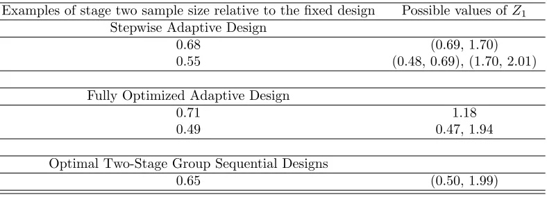
2.1 How stage 2 sample size knowledge translates into possible stage 1
results by design type for optimal designs with prior θ∼N(0,(δ/2)2),
90% power and 5% Type I error, one-sided . . . 18
3.1 Sequential Inference for Nosocomial Pneumonia (NP) Study . . . 57
3.2 Sequential Inference under Sample Space Ordering by β-Spending for
Nosocomial Pneumonia (NP) Study . . . 63
4.1 Probability π for a successful trial, individual powerπi, and expected
sample size for different design options, scenarios and strategies to
stop the trial (α=0.025 and β=0.2) with 100000 simulations. One
pri-mary and one secondary endpoint for each treatment group.
O’Brien-Fleming-type spending function for efficacy boundary for all endpoints
4.2 Probability π for a successful trial, individual power πi and expected
sample size for different design options and scenarios (α=0.025 and
β=0.2) with 100000 simulations. One primary and one secondary
endpoint for each treatment group. O’Brien-Fleming-type spending
function for efficacy boundary and Pocock-type spending function for
List of Figures
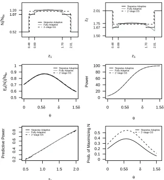
2.1 Total sample sizeN/Nf ix(top left) and the boundary value (top right)
at the second stage for designs optimized for prior θ ∼N(δ/2,(δ/2)2)
with 90% power and 5% Type I error, one-sided; expected sample size
(middle left), power (middle right), predictive power (bottom left),
probability of maximizing N after first interim analysis (bottom right)
over a range of θ for the design optimized for prior θ∼N(δ/2,(δ/2)2). 17
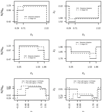
2.2 Total sample size N/Nf ix and the boundary value at the second stage
for designs optimized for prior θ ∼ N(0,(δ/2)2) (top), for prior θ ∼
N(δ,(δ/2)2) (middle), and for priorθ ∼N(δ/2,(2δ)2) vs. θ ∼N(δ/2,(δ/2)2)
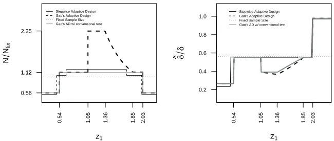
2.3 Total sample sizeN/Nf ix (left) and observed treatment effect at study
boundary (right). Stepwise adaptive design and Gao’s adaptive designs
have n1/n2 = 0.5, the stepwise adaptive design is optimized for prior
θ ∼N(δ/2,(δ/2)2), and the maximum sample size for Gao’s adaptive
design can be up to double the size of the sample size for a two-stage
group sequential design to have 90% conditional power when the
first-stage test statistic fall into promising zone. . . 23
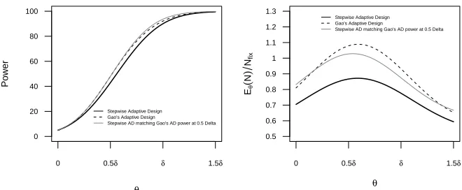
2.4 Power Curve (left) and expected sample size (right). Grey line shows
the power curve for a stepwise adaptive design which matched the
power of Gao’s adaptive design at 0.5δ. . . 24
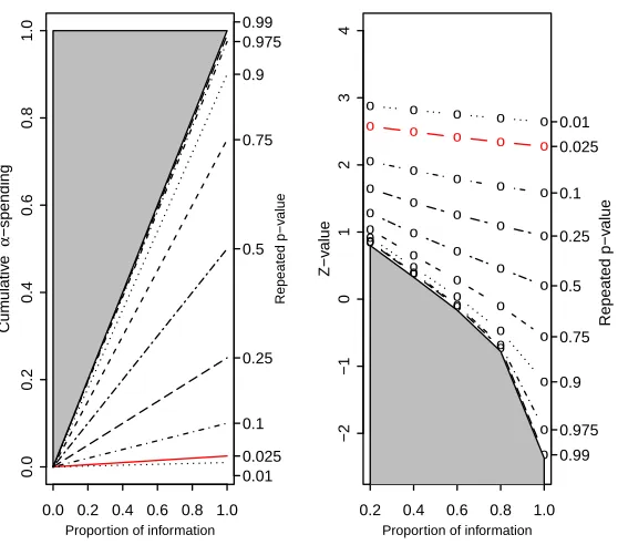
3.1 Ordering of Sample Space by total Type I error associated with the
bound: Pocock design with 5 equally spaced interim analyses. . . 39
3.2 Ordering of Sample Space by total Type I error associated with the
bound: Power spending function with ρ= 1 . . . 45
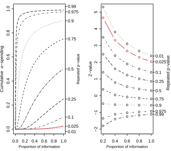
3.3 Ordering of Sample Space by total Type I error associated with the
bound: O’Brien-Fleming-type spending function . . . 46
3.4 Ordering of Sample Space by total Type I error associated with the
bound: Exponential Spending Function with ν = 0.8, which
3.5 Ordering of Sample Space by total Type I error associated with the
bound: Exponential Spending Function with ν = 0.2, which
approxi-mates Pocock boundary . . . 49
3.6 Boundaries as a function of Type I error: Exponential Spending
Func-tion with ν = 0.8, which approximates O’Brien-Fleming boundary . . 50
3.7 Ordering of Sample Space by total Type I error associated with the
bound: Power Family withρ= 1 and α0 = 0.025 . . . 53
3.8 Boundaries as a function of Type I error: Power Family with ρ = 1
and α0 = 0.025 . . . . 54
3.9 Boundaries as a function of Type II error: Exponential Spending
Func-tion withν = 0.8. The sample size is fixed as the design withα = 0.025
and β = 0.1. . . 60
3.10 Boundaries as a function of Type II error: Power Family with ρ = 1
and β0 = 0.1. The sample size is fixed as the design with α = 0.025
and β = 0.1. . . 61
4.1 Multiple testing strategy for two primary hypotheses H1, H2 and two
Chapter 1
Introduction
Clinical trials often take long time and a lot of resources to conduct. Interim
anal-yses are often performed in clinical trials because of ethical and economical reasons.
There is an ethical need to ensure that patients are not exposed to unsafe, inferior
or ineffective treatments. Early stopping may also allow highly effective medicines to
come to market faster for patients who do not have good treatment options. Early
completion can also free up resources for studies addressing other pressing medical
issues.
In recent years, the potential use of adaptive designs in clinical trials have attracted
great interest because of the potential gain of efficiency in drug development processes
(e.g., shorter duration, fewer patients). The Pharmaceutical Research and
Manufac-turers of America (PhRMA) has formed an adaptive design working group to promote
the usage of adaptive designs and related methodology (Gallo et al. (2006)). The
issues in confirmatory clinical trials planned with an adaptive design” (EMA (2007)).
The Food and Drug Administration (FDA) recently released the draft guidance on
adaptive design clinical trials and discussed various aspects of usage, considerations,
challenges of application of adaptive design trials (Food and Drug Administration
(2010)). The FDA draft guidance defines an adaptive design clinical study as “a
study that includes a prospectively planned opportunity for modification of one or
more specified aspects of the study design and hypotheses based on analysis of data
(usually interim data) from subjects in the study.” Various aspects of clinical trials
could be modified at interim analysis; these include, but are not limited to, study dose,
treatment duration, study endpoints, randomization, study design, study hypotheses,
sample size, etc.
Sample size re-estimation based on unblinded interim effect size estimates has
drawn a great deal of interest due to its permitting revision of the hypothesized
treat-ment difference from an ongoing trial while preserving the Type I error rate. When
there is uncertainty about the assumptions of treatment effect at the design stage, it
would be valuable to check these assumptions and make a midcourse adjustment to
maintain the study power. Several adaptive design methods have been proposed to
re-estimate sample size using the observed treatment effect after an initial stage of a
clinical trial while preserving the overall Type I error at the time of the final
analy-sis (Proschan and Hunsberger (1995); Cui et al. (1999); M¨uller and Sch¨affer (2001)).
inverted to reveal the exact treatment effect at the interim analysis (Ellenberg et al.
(2006)). In Chapter 2, we propose using a step function with an inverted U-shape of
observed treatment difference for sample size re-estimation to lessen the information
on treatment effect revealed. This will be referred to as stepwise two-stage sample
size adaptation. This method applies calculation methods used for group sequential
designs. We minimize expected sample size among a class of these designs and
com-pare efficiency with the fully optimized two-stage design, optimal two-stage group
sequential design and designs based on promising conditional power. The tradeoff
between efficiency versus the improved blinding of the interim treatment effect is also
discussed.
Armitage, McPherson, and Rowe (1969) had numerically shown that repeated
testing at a fixed level at interim analyses inflates the overall Type I error rate. Group
sequential designs (Pocock (1977); O’Brien and Fleming (1979); Lan and DeMets
(1983); Jennison and Turnbull (2000); etc.) have been developed and are well accepted
to control the Type I error rate with possible early stopping to either accept or reject
the null hypothesis. P-values are often used to measure the strength of evidence
against the null hypothesis in favor of the alternative. An ordered outcome space
is required to compute a p-value. Unlike a fixed sample design, a group sequential
trial might stop early and the densities for the group sequential statistics used to
stop the trial lack a monotone likelihood ratio. There are several ways to order the
and Mehta (1984); maximum likelihood estimate (MLE) ordering by Emerson and
Fleming (1990); likelihood ratio ordering or z-score ordering by Chang (1989); score
test ordering or B-value ordering by Rosner and Tsiatis (1988); and sequential p-value
ordering by Liu and Anderson (2008a). In Chapter 3, we review the existing sample
space orderings for group sequential designs and we show the advantage of sequential
p-value ordering because this method uses the totality of the accumulating data,
taking into account the entire sample path, while the other orderings only consider
the data where the boundary was crossed or the data at the current analysis. We
show that some spending functions could not completely order the sample space
when sequential p-value ordering is used to test the null hypothesis (Type I error).
We propose a simple method to transform such a spending function to one which
can completely order a group sequential design sample space. We also extend the
sequential p-value ordering to test the alternative hypothesis (Type II error). The
two one-sided sequential p-values against the null or alternative hypothesis may be
useful for a Data Monitoring Committee (DMC) making an appropriate decision.
Much of the work on group sequential methods was developed under a single
end-point. Clinical trials often involve more than one endend-point. It is of interest to extend
the group sequential methods in the multiple endpoint/testing context. Less
litera-ture is available for this topic. In Chapter 4, we propose to apply sequential p-values
methods to closed test based multiple testing procedures to control the familywise
study power and expected sample size of a group sequential design with two primary
and two secondary endpoints. We study the operating characteristics of this design
under many different scenarios of design parameters and using different spending
Chapter 2
Stepwise two-stage sample size
adaptation
2.1
Introduction
Different adaptive design methods have been proposed to modify sample size based
on unblinded results from interim analysis while preserving the Type I error rate.
Proschan and Hunsberger (1995) proposed a two-stage adaptive design to re-estimate
second-stage sample size based on conditional power assuming the observed interim
treatment effect. Liu and Chi (2001) varied this approach based on conditional power
computed under the minimum treatment effect of interest. Anderson and Liu (2004)
showed that the latter approach improves efficiency compared to the former approach.
and Sch¨affer (2001) showed the overall Type I error can be preserved unconditionally
under any general adaptive change given that the conditional Type I error is preserved.
Posch et al. (2003) investigated an ‘optimal’ reassessment rule which minimizes the
expected sample size over some set of fixed alternatives with an overall desired power
at the minimum treatment effect of interest. They described the optimal second-stage
sample size as a polynomial function of the first-stage test statistic given the stopping
boundaries and preplanned weights of the group sequential designs. Lokhnygina and
Tsiatis (2008) proposed a fully optimized, decision-theoretic two-stage adaptive group
sequential design to achieve the minimum expected sample size averaged over a normal
prior or some fixed alternatives for the treatment effect. This optimal two-stage design
is adaptive in that the sample size at the second stage depends on the data from the
first stage. They used backward induction algorithm to solve for a Bayesian sequential
decision problem following Schmitz (1993), and Barber and Jennison (2002).
The re-estimated sample size in the second stage from these adaptive designs is a
continuous function of the observed test statistic (treatment effect) at the first interim
analysis. Given the study design and the second-stage sample size, the treatment
effect at the interim analysis might be back-calculated. This is generally considered
a poor feature of these designs (Ellenberg et al. (2006)). One way to reduce the
information revealed about the treatment effect in the interim analysis is to make the
second-stage sample size a step function of interim treatment effect, i.e., to provide
In this paper, we outline a pre-specified two-stage design with a limited set of
stage two sample size possibilities and minimizing the expected sample size under
the assumption of a normal prior for the treatment effect. We compare this design
with the fully optimized two-stage adaptive design (Lokhnygina and Tsiatis (2008)),
optimal two-stage group sequential designs (Anderson (2007)) and designs based on
promising conditional power (Gao et al. (2008), Mehta and Pocock (2011)). We
conclude with a discussion in the final section.
2.2
A two-stage design with a limited set of stage
two sample size possibilities
Assume X1, X2, . . . are independent and identically distributed with a Normal
(θ,1) distribution. Let θ represent the single parameter of interest, which is the
treatment effect in our case. Assume n1 is the first-stage sample size and there are
m−1 possible stage two sample sizes at the first interim analysis. Fori= 1,2, . . . , m,
ni is a sequence of positive integers and denote
Zi = ni X
j=1 Xi/
√
ni.
We will assume n1 < ni, i = 2,3, . . . , m, but that otherwise these numbers are not
ordered in any particular way. The amount of statistical information about θ after
1≤nj ≤ni we have
E{Zi} = θ
p
Ii, (2.2.1)
Cov(Zj, Zi) =
q
Ij/Ii (2.2.2)
Jennison and Turnbull (2000) refer to this as the ‘canonical form’ when used with
group sequential designs where n1 < n2 < . . . < nm. It is the asymptotic form for
a broad variety of group sequential designs with endpoints having different
distribu-tions.
We consider two-stage designs both since the two-stage design should be simple
to implement and because it minimizes what is revealed about the interim treatment
effect. For some initial sample size n1 we compute a test statistic Z1 and for some
integer m >1 we consider boundary values a1 < a2 < . . . < am. The trial is stopped
after the analysis of n1 patients for a positive efficacy finding if Z1 ≥ am, while if
Z1 < a1 the trial is stopped for futility. For i = 2,3, . . . , m, if ai−1 ≤ Z1 < ai the
trial continues to the second stage with a sample size of ni > n1, a test statistic Zi is
computed based on the mean of the entireni observations, and for some real valuebi
efficacy is established if Zi > bi. In this two-stage design setting,b1 = am. Note that
for i= 2,3, . . . , mthere is no restriction on the ordering of the ni values. If they are
all equal or if m = 2, this becomes a two-stage group sequential design.
The probability of crossing an upper bound at the first interim analysis with n1
observations is
Fori= 2,3, . . . , mthe probability of the first interim test statistic being betweenai−1
andai and then crossing the upper bound afterni observations at the second stage is
αi(θ) =Pθ{{ai−1 ≤Z1 < ai} ∩ {Zi ≥bi}}. (2.2.4)
Similarly, the probability of crossing a lower bound at the first interim analysis
with n1 observations is
β1(θ) = Pθ{Z1 < a1} (2.2.5)
Fori= 2,3, . . . , mthe probability of the first interim test statistic being betweenai−1
and ai and then failing to cross the upper boundary at the second stage afterni > n1
observations is
βi(θ) = Pθ{{ai−1 ≤Z1 < ai} ∩ {Zi < bi}}. (2.2.6)
These probabilities can be computed using group sequential design computations
as outlined in Jennison and Turnbull (2000). The total probability of crossing an
upper bound at any time is
α(θ) =
m
X
i=1
αi(θ) (2.2.7)
and the Type I error for the design is α(0). The probability of being below a lower
boundary (a1for the first interim analysis andbifor stage two analysis afternipatients
for i= 2,3, . . . , m) is
β(θ) =
m
X
i=1
βi(θ) (2.2.8)
2.3
Reparameterizing the design
The design can be parameterized by using the sample sizes and boundaries, e.g.,
ni,ai andbi, fori= 1,2, . . . , m. Our goal is to achieve the minimum expected sample
size over a range of alternatives. We will reparameterize the design here, beginning
with boundary crossing probabilities under the null hypothesis and relative sample
sizes at the different stages of the design.
The overall Type I error for the design is
α≡α(0) =
m
X
i=1
αi(0) (2.3.1)
The probability of a negative finding under the null hypothesis is
1−α =β(0) =
m
X
i=1
βi(0) (2.3.2)
Leaving ni fixed for i = 1,2, . . . , m we can map back and forth from a
parame-terization using a1 and ai, bi, i = 2,3, . . . , m, to another using α and αi(0), βi(0),
i = 2,3, . . . , m. We briefly discuss the method for doing this. First, consider the
bounds at the first stage. Since β1(0) = P{Z1 < a1} we havea1 = Φ−1(β1(0)) where
Φ−1() represents the inverse of the standard normal cumulative distribution function.
Next, note that for i= 2, . . . , m
P0{Zi < ai}= Φ(ai) = β1(0) +
i
X
j=2
(αj(0) +βj(0)) (2.3.3)
and thus
ai = Φ−1 β1(0) +
i
X
j=2
(αj(0) +βj(0))
!
Fori= 2,3, . . . , m the value of bi is a solution to the equation
βi(0) =P0{{ai−1 ≤Z1 < ai} ∩ {Zi < bi}}. (2.3.5)
where βi, ai and ai−1 are fixed. This is a standard computation for deriving group
sequential designs that is outlined in Jennison and Turnbull (2000). With the
repa-rameterization from ai and bi to αi(0) and βi(0) we now have a method of choosing
designs that control Type I error.
Next we consider sample size parameterization to control power. We let ri =
ni/n1 > 1 represent the relative increase in sample size at the second stage of the
trial based on interim results at stage 1, i = 2,3, . . . , m. The initial parameters
defining the distribution weren1, . . . , nm,a1, . . . , am,b2, . . . , bm. Note b1 =am in this
two-stage design setting. Thus, there were a total of 3m −1 parameters defining
the design. The complete reparameterization now consists of n1, α, ri, αi(0) and
βi(0), i = 2,3, . . . , m, which still has 3m−1 parameters. Any two designs with all
parameters other thann1 equal will have the same Type I error structure. The power
to reject θ= 0 when, in truth, θ =δ >0, 1−β(δ), is strictly increasing as a function
of n1 in this case. δ represents the minimal treatment difference of interest. A root
finding algorithm can find a minimum value ofn1 that provides a desired power level.
2.4
Unrestricted 2-stage designs
An appropriately selected and unrestricted parameter space can make
optimiza-tion problems particularly tractable. We develop an unrestricted reparameterizaoptimiza-tion
of the design. We assume α and β(δ) are fixed at desired levels. It may be easier to
optimize the unrestricted value n1 rather than β(δ) if power is not restricted. Note
that we are treatingn1 as a proportion of the sample size of a fixed design (nf ix) with
Type I error αand power 1-β(δ), and thus as a continuous variable rather than as an
integer value here.
We consider a real value xai and let
αi(0) =
αexp(xai)
1 +Pm
j=2exp(xaj)
(2.4.1)
i= 2,3, . . . , m. Similarly, we consider a real value xbi and let
βi(0) =
(1−α) exp(xbi)
1 +Pm
j=2exp(xbj)
(2.4.2)
i= 2,3, . . . , m. Note that
α1(0) =
α
1 +Pm
j=2exp(xaj)
, (2.4.3)
and
β1(0) =
1−α
1 +Pm
j=2exp(xbj)
, (2.4.4)
Finally, we consider a real value xri and let ri = 1 + exp(xri), i = 2,3, . . . , m.
Now our parameter space consists of fixed values αand β(δ) and 3m−3 unrestricted
probability parameter space and then to the appropriate boundary cutoffs. A simple
optimization function such as the R nlminb function can be used to find a design to
minimize the expected sample size given a fixed Type I error, power and δ value.
2.5
Results
2.5.1
Stepwise Adaptive Design Characteristics
The fully optimized two-stage design from Lokhnygina and Tsiatis (2008) suggests
that the sample size for the second stage is an inverted ‘U’ shape curve of the test
statistic from the first stage to achieve the minimum expected sample size over a
range of alternatives. Posch et al. (2003) also suggests a similar shape of the optimal
second-stage polynomial while minimizing expected sample size averaged over some
fixed alternatives, i.e., only upsizing the trial when the treatment effect in the first
interim is an intermediate effect furthest from stage one boundaries.
In light of the inverted ‘U’ shape curve from Lokhnygina and Tsiatis (2008) design,
we present the stepwise adaptive design, which is an optimal design with two choices
of second-stage sample sizes with m = 4. We set the choice of second-stage sample
size to one value when the first-stage test statistic is close to either the futility bound
or efficacy bound at the first interim, i.e.,n2 =n4. The other choice of sample size is
chosen when the first-stage test statistic falls into an intermediate region away from
that is not particularly close to the null or alternate hypothesis effect size. This feature
can further blind the treatment effect at the first interim analysis. The expected
sample size was integrated over a normal prior distribution for θ with mean and
standard deviationδ/2. The prior mean might be chosen based on the best knowledge
of the treatment effect before the trial started. The prior standard deviation might
be chosen to reflect the range of the interest. The specific choice ofδ/2 was arbitrary.
We’ll show the results later about the impact of the choice of the prior mean and
standard deviation on the optimization of the trial design. The second-stage sample
sizes and the cutoffs for selecting among stage two sample sizes were selected through
the optimization algorithm which minimizes the expected sample size. The first-stage
sample size was selected to produce the desired power 1−β(δ).
Figure 2.1 (top) shows the stepwise adaptive design, the fully optimized
two-stage adaptive design (Lokhnygina and Tsiatis (2008)) and optimal two-two-stage group
sequential designs (Anderson (2007)). We focus on the proposed stepwise adaptive
design first. The top left figure shows total sample size N for the optimal design
expressed as a percentage of the fixed sample size design, Nf ix, as a function of the
standardized statistic at first interim analysis, Z1. The top right figure shows the
boundary value at the second stage, Z2, as a function of Z1. For error probabilities
α = 0.05 and β = 0.1, Nf ix = (1.64 + 1.28)/δ2 and the boundary for a one stage
study would be Φ−1(0.95) = 1.64. In this two-stage design, the first interim analysis
is less than 0.48 then the trial will stop for futility. If the standardized test statistic
Z1 exceeds 2.01, the trial will stop for efficacy. If the standardized test statistic Z1
falls into the region [0.69, 1.70], the final total sample size would be 1.20Nf ix and the
second-stage boundary would be 1.75. Otherwise, if the standardized test statisticZ1
falls into the other area of the continuation region, the final total sample size would
be 1.07Nf ix. and the second-stage boundary is 1.67.
While Figure 2.1 (top) also compares the study designs from this stepwise adaptive
design with the fully optimized two-stage adaptive design (Lokhnygina and Tsiatis
(2008)) and optimal two-stage group sequential designs (Anderson (2007)). The
step-wise adaptive design gives two choices of second-stage sample size: the total sample
size close to the sample size from a fixed design when the first interim test
statis-tic is close to the futility bound or efficacy bound; the total sample size increases
about 20% compared to the sample size from a fixed design when the first interim
test statistic is intermediate. The stepwise adaptive design is simplified compared to
the fully optimized two-stage adaptive design. Comparing to the optimal two-stage
group sequential design, the stepwise adaptive design has the sample size and
bound-ary close to the fixed sample size design when the interim test statistic is close to the
first-stage boundaries. The maximum sample size and corresponding second-stage
boundary from stepwise adaptive design is a bit higher compared to group sequential
design but not much higher. Knowing the sample size adaptation following stage 1
trans-z1
N
Nfi
x
0.48 0.69 1.70 2.01
0.52 1.07 1.07 1.20 Stepwise Adaptive Fully Adaptive 2−stage GS z1 z2
0.48 0.69 1.70 2.01
1.50 1.67 1.75 2.01 Stepwise Adaptive Fully Adaptive 2−stage GS θ Eθ ( N ) Nfi x
0 0.5δ δ 1.5δ
0.5 0.6 0.7 0.8 0.9 1 Stepwise Adaptive Fully Adaptive 2−stage GS θ P o w e r
0 0.5δ δ 1.5δ
0 20 40 60 80 100 Stepwise Adaptive Fully Adaptive 2−stage GS
0.5 1.0 1.5 2.0
0.2 0.4 0.6 0.8 z1 Predictiv e P o w
er Stepwise Adaptive Fully Adaptive 2−stage GS
θ
Prob
. of Maximizing N
0 0.5δ δ 1.5δ
0 0.1 0.2 0.3 0.4
0.5 Stepwise Adaptive2−stage GS
Figure 2.1: Total sample size N/Nf ix (top left) and the boundary value (top right)
at the second stage for designs optimized for prior θ ∼ N(δ/2,(δ/2)2) with 90%
power and 5% Type I error, one-sided; expected sample size (middle left), power (middle right), predictive power (bottom left), probability of maximizing N after first
interim analysis (bottom right) over a range of θ for the design optimized for prior
Table 2.1: How stage 2 sample size knowledge translates into possible stage 1 results
by design type for optimal designs with prior θ ∼ N(0,(δ/2)2), 90% power and 5%
Type I error, one-sided
Examples of stage two sample size relative to the fixed design Possible values ofZ1 Stepwise Adaptive Design
0.68 (0.69, 1.70)
0.55 (0.48, 0.69), (1.70, 2.01)
Fully Optimized Adaptive Design
0.71 1.18
0.49 0.47, 1.94
Optimal Two-Stage Group Sequential Designs
0.65 (0.50, 1.99)
lated into an approximate range for the interim observed treatment effect. Table
2.1 shows the examples of the range of possible Z-values that correspond to different
known stage 2 sample sizes.
Figure 2.1 (middle and bottom) compares the expected sample size, overall power,
and predictive power of this stepwise adaptive design with the fully optimized
two-stage adaptive design and optimal two-two-stage group sequential designs. The stepwise
adaptive design had nearly identical expected sample size and overall power over a
range of alternatives compared to the fully optimized two-stage adaptive design and
optimal two-stage group sequential designs. Predictive power is defined as a weighted
average of conditional power (conditioning on the first-stage test statistic) with prior
θ ∼N(δ/2,(δ/2)2). The stepwise adaptive design and fully optimized adaptive design
have higher predictive power when the first-stage test statistic is close to the upper
to the lower futility bound compared to optimal two-stage group sequential design.
We also compare the probability of maximizing sample size for the stepwise adaptive
design and the optimal two-stage group sequential design. The stepwise adaptive
design has a lower probability of requiring the maximum total sample size compared
to the optimal two-stage group sequential design as shown in Figure 2.1 (bottom
right), though the maximum sample size is a bit larger for the stepwise adaptive
design.
The designs shown above are based on a prior distribution of θ ∼N(δ/2,(δ/2)2),
which is the situation when the investigator has some prior information and is neutral
on treatment effect between the null and alternative hypothesis. Early Phase II
development of experimental drugs might fit this situation. We also explored the
stepwise adaptive design which uses different prior distribution. Figure 2.2 (top)
shows the design with prior θ ∼ N(0,(δ/2)2) and Figure 2.2 (middle) shows the
design with prior θ ∼ N(δ,(δ/2)2). With prior mean =0, the experimenter does
not have much confidence in the treatment effect; the stepwise adaptive design only
increases the sample size when the interim statistics looks promising. With prior
mean =δ, the experimenter has more confidence in the treatment effect, the stepwise
adaptive design only increases the sample size when the interim test statistic does
not look promising. We also investigate the impact of a flatter prior distribution on
the design. Figure 2.2 (bottom) shows the design with prior θ ∼ N(δ/2,(2δ)2) vs.
region and an earlier first interim analysis which would be conducted after 0.29Nf ix
observations. This is inconsistent with common recommendation of conducting the
first interim analysis at around 50% information time. This suggests that the time
to adapt also depends on how much prior information we have. For many trials
with delayed endpoints, the only possible time for adaptation would be at early time
points.
2.5.2
Stepwise Adaptive Design Compares with Designs Based
on Promising Conditional Power
Chen et al. (2004) showed that the conventional test could be performed without
inflating the Type I error if one increased the sample size only when interim results
were promising, which was defined as conditional power of 50 percent or greater. Gao
et al. (2008) and Mehta and Pocock (2011) further extended this idea to a broader
range of promising zones in which the sample size may be increased up to an upper
bound based on conditional power and the conventional tests may be applied without
inflating Type I error.
Define z1 as the first-stage test statistic, ˜n2 as the incremental sample size at
the second stage, and ˆδ1 as the observed treatment effect at stage 1. Mehta and
Pocock (2011) partitioned the conditional power value,CPδˆ1 (z1, ˜n2), into three zones:
unfavorable zone, promising zone and favorable zone. CPδˆ1 (z1, ˜n2) < CPmin defined
z1
N
Nfi
x
0.29 0.71 2.22 0.42 0.99 1.23 Stepwise Adaptive 2−stage GS z1 z2
0.29 0.71 2.22 1.52 1.68 2.22 Stepwise Adaptive 2−stage GS z1 N Nfi x
0.25 1.53 1.96 0.47 0.97 1.22 Stepwise Adaptive 2−stage GS z1 z2
0.25 1.53 1.96 1.70 1.85 1.96 Stepwise Adaptive 2−stage GS z1 N Nfi x
−0.15 0.48 0.69 1.70 2.01
0.29 0.52 1.07 1.07 1.20
Prior with sigma = 0.5*Delta Prior with sigma = 2*Delta
z1
z2
−0.15 0.48 0.69 1.70 2.01
1.67 1.75 2.01
Prior with sigma = 0.5*Delta Prior with sigma = 2*Delta
Figure 2.2: Total sample size N/Nf ix and the boundary value at the second stage
for designs optimized for prior θ ∼ N(0,(δ/2)2) (top), for prior θ ∼ N(δ,(δ/2)2)
(middle), and for prior θ ∼N(δ/2,(2δ)2) vs. θ∼ N(δ/2,(δ/2)2) (bottom) with 90%
that the interim result is so disappointing that it is not worth increasing the sample
size. CPmin ≤CPδˆ1(z1,n˜2)<1−β defined the promising zone, with results that are
not disappointing but not good enough for the conditional power to equal or exceed
the unconditional power specified at the design stage. CPδˆ1(z1,n˜2) ≥ 1−β defined
the favorable zone, in which the interim results are favorable. This approach can be
extended to a two-stage group sequential design with possible early stopping at stage
one. We present the stepwise adaptive design with the constraint of n1/n2 = 0.5
and Gao’s method on two-stage group design where nmax/n2 = 2, n1/n2 = 0.5 and
1−β = 0.9 in Figure 2.3 (left). The sample size in Gao’s adaptive design is up to
double the sample size of the two-stage group sequential design when the interim test
statistic is in the promising zone. We also compare the second-stage critical values
for different designs. Mehta and Pocock (2011) mentioned that the Type I error was
preserved even when the conventional test was performed, and suggested using the
second-stage boundary of the unfavorable zone/the favorable zone for the promising
zone. Figure 2.3 (right) shows the observed treatment effect at the study boundary
when the trial is stopped for designs with α = 0.05. The observed treatment effect
at the boundary of Gao’s adaptive design is much smaller than the stepwise adaptive
design due to the big sample size increase in the promising zone even if we use the
conventional test. Figure 2.4 show the power and expected sample size from the
stepwise adaptive and Gao’s adaptive design. When we match the power of the
z1
N
Nfi
x
0.54 1.05 1.36 1.85 2.03
0.56 1.12 1.12 2.25
Stepwise Adaptive Design Gao's Adaptive Design Fixed Sample Size Gao's AD w/ conventional test
z1
δ
^ δ
0.54 1.05 1.36 1.85 2.03
0.2 0.4 0.6 0.8 1.0
Stepwise Adaptive Design Gao's Adaptive Design Fixed Sample Size Gao's AD w/ conventional test
Figure 2.3: Total sample size N/Nf ix (left) and observed treatment effect at study
boundary (right). Stepwise adaptive design and Gao’s adaptive designs haven1/n2 =
0.5, the stepwise adaptive design is optimized for prior θ ∼ N(δ/2,(δ/2)2), and the
maximum sample size for Gao’s adaptive design can be up to double the size of the sample size for a two-stage group sequential design to have 90% conditional power when the first-stage test statistic fall into promising zone.
the stepwise adaptive design if the true mean is δ and the expected sample size is
generally smaller for the stepwise adaptive design.
2.6
Discussion
Lokhnygina and Tsiatis (2008) presented a fully optimized two-stage design that
has minimum expected sample size averaged over a range of alternatives. In this
paper, we simplified this design and presented a method to create a pre-specified
optimal two-stage design with a limited set of stage two sample size possibilities to
lessen the information revealed at the interim analysis.
In this paper, we focus the stepwise adaptive design with two choices of
second-stage sample size for the prior distribution of θ ∼ N(δ/2,(δ/2)2). We set the choice
θ
P
o
w
e
r
0 0.5δ δ 1.5δ
0 20 40 60 80 100
Stepwise Adaptive Design Gao's Adaptive Design
Stepwise AD matching Gao's AD power at 0.5 Delta
θ
Eθ
(
N
)
Nfi
x
0 0.5δ δ 1.5δ
0.5 0.6 0.7 0.8 0.9 1 1.1 1.2 1.3
Stepwise Adaptive Design Gao's Adaptive Design
Stepwise AD matching Gao's AD power at 0.5 Delta
Figure 2.4: Power Curve (left) and expected sample size (right). Grey line shows the power curve for a stepwise adaptive design which matched the power of Gao’s
adaptive design at 0.5δ.
either the futility bound or efficacy bound at the first interim analysis, i.e.,n2 =n4,
and to a different value when the first-stage test statistic falls into an intermediate
region away from the first-stage stopping boundaries,i.e., an intermediate treatment
effect is observed that is not particularly close to the null or alternate hypothesis effect
size. This feature of the design improves blinding of the interim treatment effect by
lessening the information revealed at the interim analysis. Each second-stage sample
size corresponds to one range or two ranges of the first interim analysis test statistic,
as shown in Table 2.1. If the study proceeds to the second stage with sample size of
0.68Nf ix, we know only that the standardized first-stage test statistic is between 0.69
and 1.70. If the study proceeds to the second stage with sample size of 0.55Nf ix, we
know only that the standardized first-stage test statistic is either between 0.48 and
0.69 or between 1.70 and 2.01. The fully optimized two-stage adaptive design has
of second-stage sample size. The optimal two-stage group sequential design has only
one choice of second-stage sample size and reveals the least information (only gave
one range of first-interim analysis test statistic). The stepwise adaptive design and
the optimal two-stage group sequential design therefore reveal less information about
the interim treatment effect than the fully optimized adaptive design.
We have seen that the efficiency loss from the stepwise adaptive design may be
min-imal compared to the substantially more complicated fully optimized design
(Lokhny-gina and Tsiatis (2008)). The stepwise adaptive, fully optimized adaptive designs and
optimal two-stage group sequential designs have similar expected sample size and
overall power over the range of θ. Advantages of the stepwise adaptive design over
the optimal two-stage group sequential design are that the minimum second-stage
sample size is much smaller, and the stepwise adaptive design is less likely to require
the maximum sample size compared to the optimal two-stage group sequential design.
Notice the shape of the stepwise adaptive design is not symmetric. This is also true
for the fully optimized two-stage adaptive design (Lokhnygina and Tsiatis (2008)).
This might be caused by the optimization process which requires a minimum expected
sample size for a given prior. We design a symmetric stepwise adaptive design with
equal length of continuation region when the first-stage test statistic is close to the
futility bound or efficacy bound at the first interim. We compare the expected sample
size for the current stepwise adaptive design with this symmetric stepwise adaptive
sample size design is 0.77096 compared to 0.77107 for the symmetric stepwise adaptive
design.
Levin et al. (2011) recently presented a completely pre-specified optimal adaptive
design. This design is similar to our stepwise adaptive design in that we both used step
functions. Levin et al. (2011) only considered the symmetric design and optimized the
design by assigning half the weight on the null and half the weight on the alternative
and achieved the optimization through adding more steps to the design. Our design
focuses on the design with fewer steps and minimizes the expected sample size over
a range of alternatives.
Chuang-Stein et al. (2006) pointed out that the interim treatment effect size can
be highly variable and potentially too unreliable to be used directly for sample size
re-estimation purposes. And in general, the sample size re-estimation design based
on conditional power is likely not optimized for expected sample size. Jennison and
Turnbull (2003) have demonstrated that mid-course sample size modification based
on the observed treatment effect come with the cost of efficiency when compared with
group sequential designs. The stepwise adaptive design is an extension of standard
group sequential design. This design is pre-specified at the design stage as the group
sequential design and also provides the opportunity of sample size adaptation with
great efficiency. The stepwise adaptive design provides a solution by combining the
prior information and the information within a trial.
two-stage adaptive and with optimal two-stage group sequential designs, but reveals
less information about interim treatment effect than the fully optimized adaptive
Chapter 3
Sample Space Ordering and
Inference for Group
Sequential/Adaptive Designs
3.1
Introduction
Armitage, McPherson, and Rowe (1969) numerically showed that if significance
tests at a fixed level are repeated at interim analyses, the Type I error rate (or α) is
greatly increased over the nominal level. Simple group sequential methods for a
pre-defined number of equally spaced interim analyses were developed by Pocock (1977)
Fleming (1979) designs to a class of group sequential tests, also referred as boundary
families. But the boundary family designs assume the maximum number of analyses,
K, be fixed in advance and require equally spaced interim analyses. Lan and DeMets
(1983) suggested an alternative method to construct discrete sequential boundaries
by using α-spending functions. The boundary at a decision time is determined by
α(t), where t is the timing of the interim analysis, which is also called information
time. Information time t is defined as Ii/Imax for i = 1, . . . , K, where Ii is the
statistical information at analysis iand Imax represents the maximum planned
infor-mation at the time of design. Kim and DeMets (1987) and Hwang, Shih, and DeCani
(1990) individually extended the method of Lan and DeMets (1983) to a general
one-parameter family of α-spending functions, α(t;γ) = α×hγ(t), where the parameter
γ specifies the rate of α-spending. The function h(t) is increasing in t ∈ (0,1) with
h(0) = 0 and h(t) = 1 for t ≥ 1. Pampallona, Tsiatis, and Kim (2001) extended
the Type I error spending method of Lan and DeMets (1983) by incorporating an
analogous Type II error (or β) spending function for interim analyses to test futility.
Anderson and Clark (2010) discussed additional one- and two-parameter spending
families. Their two- or three-parameter spending function families provide additional
flexibility to customize the shape of spending functions to fit more than one desired
critical value. The spending function approach has become common because of its
flexibility in accommodating unequally-spaced analyses and allowing some leeway in
of treatment effects. This is compared to boundary families which require a fixed total
number of analyses, generally performed at equally-spaced intervals. The boundaries
constructed by α- andβ- spending functions are determined by the past and current
information times but not by future information times, and not by the total number
of analyses. These are the properties of the spending function approach that allow
flexibility in resetting timing of analyses during the course of the trial.
Group sequential designs with asymmetrical boundaries permit clinical trial
stop-ping for efficacy when the interim results cross the upper boundaries or stopstop-ping for
futility when the interim results cross the lower boundaries. Boundaries of the group
sequential design define the acceptance or rejection of the null hypothesis of the group
sequential test on their own, however the boundaries do not provide additional
in-formation about the relative strength of the evidence to reject the null hypothesis.
Fori= 1,2, . . . , K, letZi be the test statistic against the null hypothesis H0 in favor
of the alternative hypothesis H1 at analysis i. Let Ci be the continuation region at
analysis i and CK =∅. Ω is the sample space defined by a classical group sequential
design, that is, the set of all pairs (i, zi) wherezi ∈/ Ci so that the test can terminate at
stageiwith (T, ZT) = (i, zi). A p-value for testingH0 can be stated as the probability
under the null hypothesis of obtaining (i, zi) as extreme or more extreme than the
observed (i∗, zi∗), where “extreme” refers to the ordering of Ω. A fixed sample design
(with no monitoring) has unique ordering of the sample space under the normality
0 as z → ∞, and the p-value converges to 1 as z → −∞ for a fixed sample design.
But this is not the case for a group sequential trial. Since the number of observations
varies between different stages, there are many ways to order the possible outcomes.
We start with a brief review of the basic concepts of group sequential testing
and existing sample space orderings for group sequential designs, including
stage-wise ordering by Tsiatis, Rosner and Mehta (1984); maximum likelihood estimate
(MLE) ordering by Emerson and Fleming (1990); likelihood ratio ordering or z-score
ordering by Chang (1989); score test ordering or B-value ordering by Rosner and
Tsiatis (1988), and sequential p-value ordering by Liu and Anderson (2008a). We
prefer to use sequential p-value ordering because this method uses the totality of
the accumulating data which takes into account the entire sample path, while the
other orderings only consider the data where the boundary was crossed or the data
at the current analysis. We will show that spending functions with the form of
α(t) = α×h(t) do not completely order the sample space using the power spending
function as an example. This has the disadvantage that there is often a broad range
of the sample space at an interim analysis where the p-value is 1. The exponential
spending function from Anderson and Clark (2010), αe(t;ν) = αt
−ν
, has a different
form from most commonly used spending functions. We will define what we mean
by the complete ordering of a group sequential sample space and show that a
Wang-Tsiatis boundary family or an exponential spending function family or Lan-DeMets
propose a simple method to transform a spending function to a completely ordered
sample space when using the sequential p-value ordering, a power spending function
will be used as an example. This method is also extended to β-spending functions
for p-values to reject the alternate hypothesis. We’ll then give examples to illustrate
our approach.
3.2
Review of Group Sequential Testing
Consider a group sequential trial with K > 1 analyses which generates the
se-quence of test statistics Z1, Z2, . . . , ZK. Let θ represent the single parameter of
inter-est, which is the treatment effect in our case. The amount of statistical information
about θ at analysis i is denoted by Ii, i = 1,2, . . . , K, with 0 < I1 < I2 < . . . < IK.
In many situations Ii is proportional to the number of observations (or events) at
interim analysis i, i = 1,2, . . . , K. Assume that the distribution of test statistics
Z1, Z2, . . . , ZK for the K analyses follows a multivariate normal distribution with
E{Zi} = θ
p
Ii, (3.2.1)
Cov(Zj, Zi) =
q
Ij/Ii (3.2.2)
for 1≤j ≤i≤K. Jennison and Turnbull (2000) refer to this as the ‘canonical form’
for group sequential designs.
We consider testing the null hypothesisH0 :θ = 0 against the alternativeH1 :θ=
LetCi be defined as the continuation region at stagei,i.e.,Ci =Tij=1{aj ≤Zj < bj},
for i= 1, . . . , K−1. Note thatCK =∅ withaK =bK. Let ai be the lower boundary
and it is also called the futility boundary. Letbi be the upper boundary and it is also
called the efficacy boundary. Fori= 1, . . . , K−1, the trial is stopped for efficacy at
the ith interim analysis to reject H0 if Zi ≥ bi, is stopped for futility to reject H1 if
Zi < ai, and continues if ai ≤ Zi < bi. At the final analysis, the null hypothesis H0
is rejected if ZK ≥bK.
First, we consider a binding lower boundary, i.e., the trial must be stopped once
either the upper or the lower boundary is crossed. For i = 1, . . . , K, the probability
of crossing an upper bound at analysis i without previously crossing any bound for
any θ is
αi(θ) = Pθ{{Zi ≥bi} i−1 \
j=1
{aj ≤Zj < bj}} (3.2.3)
The value αi(0) is commonly referred to as the amount of α (Type I error) spent at
analysis i, for i = 1, . . . , K. The total Type I error for a trial will be denoted by
α(0) ≡PK
i=1αi(0).
For i = 1, . . . , K, the probability of crossing a lower bound at analysis i without
previously crossing any bound for any θ is
βi(θ) =Pθ{{Zi < ai} i−1 \
j=1
{aj ≤Zj < bj}}. (3.2.4)
The valueβi(δ) is commonly referred to as the amount ofβ (Type II error) spent at
analysis i, for i = 1, . . . , K. The total Type II error for a trial will be denoted by
β(δ)≡PK
Sometimes the futility boundary is considered just a guideline, which means that a
study can continue even though the futility boundary has been crossed withZi < ai,
for i = 1, . . . , K −1. The futility boundaries are then called non-binding futility
boundaries. In this case, the boundaries ai and bi are defined by replacing αi(θ) in
(3.2.3) with α+i (θ) where
α+i (θ) =Pθ{{Zi ≥bi} i−1 \
j=1
{Zj < bj}} (3.2.5)
and
α+(θ)≡
K
X
i=1
α+i (θ). (3.2.6)
.
3.3
Review of Sample Space Ordering
It is important to provide the strength of evidence to reject the null hypothesisH0 :
θ = 0 after a trial is complete or even during a trial. For a trial with no monitoring,
the p-value should be uniformly distributed under H0, i.e., P r{p-value ≤ p} = p
for all 0 ≤ p ≤ 1. As the z-value increases from −∞ to ∞, P r(Z > z) decreases
from 1 to 0 for a one-sided test. For a group sequential trial, a p-value for testing
H0 can be stated as obtaining (i, zi) as extreme or more extreme than the observed
(i∗, zi∗), where “extreme” refers to the ordering of the sample space Ω, which is the
(2006) summarized four sample space orderings by using the value of (i, zi) at trial
termination:
A. Stage-wise ordering by Tsiatis, Rosner and Mehta (1984), (i0, zi0)(i, zi) if (1)
i0 =i and zi0 ≥zi (2) i0 < i and zi0 ≥bi0 (3) i0 > i and zi ≤ai.
B. Maximum likelihood estimate (MLE) ordering by Emerson and Fleming (1990),
(i0, zi0)(i, zi) if z0i/
√
Ii0 > zi/
√
Ii, whereIi is the statistical information.
C. Likelihood ratio ordering or z-score ordering by Chang (1989), (i0, z0i)(i, zi)
if zi0 > zi.
D. Score test ordering or B-value ordering by Rosner and Tsiatis (1988), (i0, zi0)
(i, zi) if zi0
√
Ii0 > zi
√
Ii.
For MLE, z-score, and B-value ordering, the p-value depends on the information
levels or group sizes beyond the observed stopping stage T = τ, while stage-wise
ordering has the property that the p-value does not depend on the information
lev-els or group sizes beyond the observed stopping stage T = τ. Stage-wise ordering
automatically ensures that the p-value is less than the significance level α of the
group sequential test if and only if H0 is rejected. Jennison and Turnbull (2000)
and Proschan, Lan and Wittes (2006) recommended stage-wise ordering. However,
stage-wise ordering also has limitations: (1) Stage-wise ordering does not provide a
p-value when the test statistic has not crossed either boundary. (2) Stage-wise
order-ing does not provide final analysis for data over-runnorder-ing, which might happen due to
the interim analysis (although this has been dealt with by Whitehead (1992)). (3)
When a test statistic is on an interim boundary, stage-wise ordering rejects the null
hypothesis at a significance level less than α. (4) A stage-wise p-value can not be
arbitrarily small after the first interim analysis, even if the test statistic is big or
evidence to reject the null is strong;i.e., the p-value for crossing at an analysis after
the first interim is always larger than the nominal p-value for a case where the first
interim bound is crossed.
Liu and Anderson (2008a) introduced an extended group sequential design (EGS
design), which is a group sequential design with the stopping time τ, taking values
of 1,2, . . . , K. τ may precede, coincide with, or exceed the boundary crossing time.
An EGS test is defined as positive if any interim or final efficacy bound is crossed,
which corresponds to the event SK
i=1[{τ =i}
T Si
j=1{Zj ≥ bj}] occurs. For an EGS
test indexed by a parameter µ∈(0,1), there existbi(µ) for i= 1,2, . . . , K, such that
P0{Z1 ≥b1(µ) [
Z2 ≥b2(µ) [
. . .[ZK ≥bK(µ)}=µ.
The class of boundaries indexed by µ∈(0,1) is defined as a well-ordered class if the
boundary bi(µ) is continuous and decreasing in µ and converges to ∞ as µ → 0 for
any i= 1,2, . . . , K.
Liu and Anderson (2008a) considered ordering the sample space using the totality
of the accumulating data. For any sample path ω = {τ;Z1, . . . , Zτ}, a repeated
is defined as pi = min1≤j≤i{µˆ(j)}. The final sequential p-value is defined as
pτ = min{µˆ(i) :i= 1, . . . , τ}.
Any two sample paths, ω0 and ω00, are said to follow the order if and only if their
final p-values, p0τ0 and p00τ00, follow the order of p0τ0 ≥ p00τ00. If ω0 ω00 and ω00 ω000,
then ω0 ω000. Thus the ordering is well defined.
The fundamental difference between Liu and Anderson (2008a) sequential p-value
ordering and other orderings including stage-wise, MLE, z-value, and B-value ordering
is that the sequential p-value ordering uses the totality of the accumulating data
which takes into account the entire sample path ω ={τ;Z1, . . . , Zτ}, while the other
orderings only consider the data where the boundary was crossed {τ;Zτ} or at the
most recent analysis. Liu and Anderson (2008a) summarized several features of the
sequential p-values: (a) The final p-value, pτ, adheres to the ITT principle that
all available data are analyzed; (b) sample paths reaching the same boundary have
identical p-values; and (c) pτ is always significant if the significance boundary is
crossed at any stage, not requiring Zτ ≥ bτ. We prefer to use sequential p-value
ordering from Liu and Anderson (2008a) because this method uses the totality of the
accumulating data and does not reverse inference once it is made.
3.4
Complete Ordering of Sample Space
To completely order the sample space as the fixed sample design, we define the
decreasing in µ, converging to ∞ as µ → 0, and converging to −∞ as µ → 1 for
any i = 1, . . . , K for a group sequential trial. A completely ordered sample space is
a well ordered sample space, but the reverse is not necessarily true. A sample space
can be well ordered without the boundary converging to −∞ asµ→1 for at least 1
i∈1, . . . , K for a group sequential trial.
The Pocock design from the boundary families is an example of complete ordering
of sample space based on a sequential p-value ordering. The sample space in the
boundary scale has complete coverage from −∞ to +∞ in the z-value scale for any
i = 1, . . . , K. And similarly, the sample space has complete coverage from 0 to 1 in
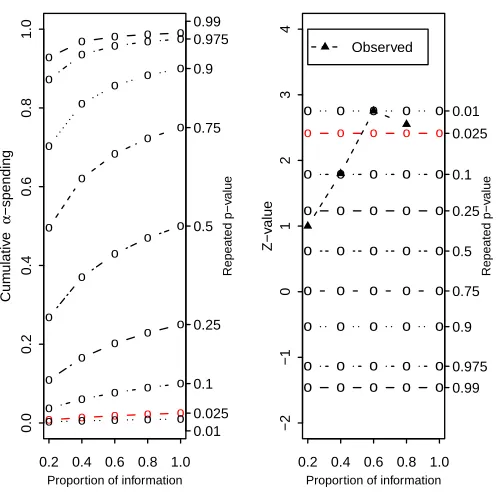
the probability scale for any i = 1, . . . , K. Figure 3.1 gives an example of a Pocock
design with 5 analyses. At the 3rd analysis, the test statistic crossed the boundary
for the pre-specified α=.025. The trial continued after the 3rd interim analysis and
stopped at the 4th interim analysis to collect more safety data. The repeated p-values
were 0.337, 0.098, 0.010, and 0.018, respectively. The sequential p-values were 0.337,
0.098, 0.010, and 0.010. The final sequential p-value was 0.010.
Boundary family tests, e.g., the Wang-Tsiatis family, including Pocock,
O’Brien-Fleming boundary, produce completely ordered sample spaces when using sequential
p-values to order the sample space. But the reduced flexibility of the boundary
fam-ily tests prevents their broader application in real situations, since change the timing
of interim analyses during the trial will result in changing the bounds already used.
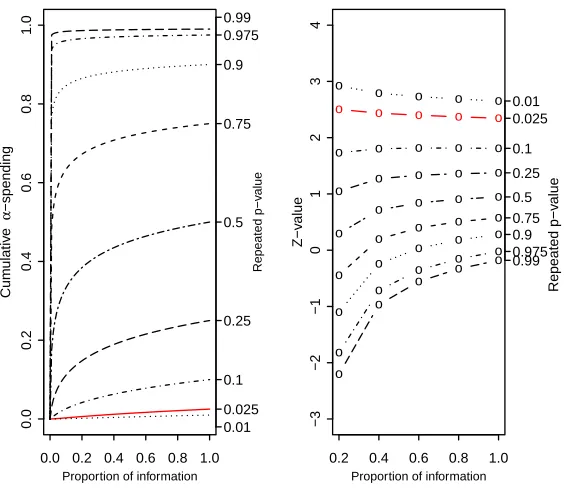
flexibil-o o o o o
0.2 0.4 0.6 0.8 1.0
0.0 0.2 0.4 0.6 0.8 1.0 0.01 0.025 0.1 0.25 0.5 0.75 0.9 0.975 0.99 Repeated p−v alue
Proportion of information
Cum
ulativ
e
α
−spending
o o o o o o o
o o o o o o o o o o o o o o o o o o o o o o o o
o o o o o
o o o o
o o o o o
0.2 0.4 0.6 0.8 1.0
−2 −1 0 1 2 3 4 0.99 0.975 0.9 0.75 0.5 0.25 0.1 0.025 0.01 Repeated p−v alue
Proportion of information
Z−v
alue
o o o o o
o o o o o
o o o o o
o o o o o
o o o o o
o o o o o
o o o o o
o o o o o
Observed
ity in changing the timing of interim analyses while keeping intact the bounds used
before. Lan and DeMets (1983) introduced spending functions to approximate the
Pocock boundary (α(t) =α(1 + log(1 + (e−1)t))) and the O’Brien-Fleming
bound-ary (α(t) = 2(1−Φ(Φ−1(1√−α/2)
t ))). Kim and DeMets (1987) introduced a spending
function based on the power function (α(t, ρ) = αtρ). Hwang, Shih, and DeCani
(1990) proposed a general one-parameter spending function to construct customized
group sequential boundaries (α(t, γ) = α11−−expexp((−−γtγ))). Anderson and Clark (2010)
introduced an exponential spending function α(t) = αt−ν and a general spending
function α(t;ν) = 2(1−F(F−1√(1−α)
tν )) (Equation 10 in Anderson and Clark (2010)).
Both O’Brien-Fleming-type spending function and the exponential spending function
are special cases of equation 10 of Anderson and Clark (2010). With the exception of
the exponential family and O’Brien-Fleming-type spending function, other spending
functions have the form α(t) = α×h(t) with t ∈(0,1) as the timing of the interim
analysis. We attempt to order a sample space by using spending functions as follows:
set up a spending function for each α level, compute corresponding bounds for each
interim, if an interim or final analysis crosses a bound, it is significant at that level.
We set significance by the ’most significant’ bound reached. This will require that the
spending function produces ordered sets of bounds as we have seen for the Pocock
de-sign where no bounds crossed others. Theorem 1 below gives sufficient conditions for
well ordered sample space and shows that the spending functions likeα(t) =α×h(t)