Investigate Stick-Slip Intervals With One Equation Of Motion And Analyse The Effect Of The Friction Noise

96

Investigate Stick-Slip Intervals with One Equation

Of Motion And Analyse The Effect Of The Friction

Noise

Ammar A. Yousif Mohammed, InzarulfaishamAbd Rahim

ABSTRACT: An attempted to understand the noise generated during the car brake was led the researcher to search for oscillation systems that represent the brake disc-pad.They were found that the oscillation between the disc and the padduring the noise generated wereself-sustained stick-slip oscillations and can be present in a one degree of freedom. In this article an attempted was investigated to solve the stick-slip oscillation by MATLAB software with one mathematical equation only instead of using three separated equation resultedfrom different three oscillation equation condition interval. Find out the sign function had made this method possible. However, stick-slip oscillation forone degree of freedomwas solved in this paper by using this method. Study of the effect of changing the dynamic properties was investigated also to predict the noise generatesby changing these parameters. The contact interaction between mass and the belt was solved to find out the relation between the friction andthe relative velocity. The relative velocity curve was conducted through solving the system frictionequation by means of numerical time integration method ODE45. Friction-relative velocity values were used later inside ABAQUS software with beam on rotating rigid disc with different contact angle and condition. This study investigates the effect of the friction on the noise generated from brake at low frequency. The vibration responses showed that the friction relative velocity ratio is responsible for the separation of the system amplitude value. Changing the contact angle could change the noise generated and presented higher fundamental frequency. As a result, this method was approved to be correct method to study stick- slip phenomena.

Keywords:stick-slip, natural frequency, squeal, contact angle, rigid body dynamic, runge-kutta method

————————————————————

1 INTRODUCTION

Stick-slip is associated with the different between kinetic and static friction coefficient, Martins et al.[1]. The compound word stick–slipwas first coined by Bowden and Leben [2]at University of Cambridge.The stick-slip is the reason of the noise at the final stage of braking, Pilipchuk and Tan [3].Since the friction have two coefficients then the resulting motion possesses also a non-smooth behavior.The nature of stick-slip response is also dependent on the ratio of friction coefficients μ = μk/μs at the sliding interface [4]. This type of motion was also observed in non-linearity systems that have a dry friction,Popp[5]. It is reported that the building during earthquake showing a stick–slip motion, S. Nagarajaiah [6].Analysis of stick-slip motions has a fascinated researchers for several decades, starting from Den Hartog’s [7] formulateof a single-degree-of-freedom system with combined Coulomb and viscous friction elements.Usually the oscillator wasmodelled as a lumped mass, which slides on a moving belt and is attached by elastic and a dissipative element to the inertial surroundings.

This classical model showeda surprising effect, thus though thepresence of friction and the steady-state may be linearly unstable if the sliding friction characteristic is declining. Brake creep/groan takes place due to a change in the brake pressure leading to stick slip friction excitations between rotor and disc under very low speeds. Groan may also occur on brake application, as reported by Brecht [8]; it typically can be a long event for brake release on takeoff and short for vehicle braking to stop.Cao et al. [9] simulation showed that groan occurs most readily under the lowest speeds and lightest brake pedal release. There is also clear dependence on road gradient, and under certain conditions, it may occur in both manual and automatic transmissions.For instance, abdelhamid [10] suggested a class of creep/groan problems where both brake and axle resonate in virtually the same frequency band. Driving conditions (slow take off, slow stop, etc.) may lead to relative motions between brake pad and disc having stick-slip orbits, steady sliding solutions or purely sticking (stationary vehicle). Abdelhamid [10] has identified multiple frequencyharmonics of the creep/groan and showednumerically the limit cycle (stick-slip orbit) behavior, in a qualitative manner, by using a nonlinear forcing function with a single mode system. Q. Feng[11] investigated a simple model to study stick-slip motion. He modeled an appropriate model that has low time cost on computer simulation. The articles compared the result of two systems before and after the model development. This study investigated that the new model is more convenience to show the random friction system and save a lot of time on computer. P. Filip [12], conduct that the variation in contact stiffness due to formation of friction layers on the interface surface and the stick–slip phenomenon due to the variation in the coefficient of friction are the reasons of the non-linearity of the motion. M North [13]said that the change of the rotor dynamic characteristics is the base of the system to generateinstabilities in both normal and frictional forces direction. Manish Paliwal et al [14] rebuildShin et al model with incorporation of the layer stiffness at the contact surface due to the formation of friction layers. By manipulationthe parameters values, the effect of layer stiffness on the instability could be _________________________

 Ammar A. Yousif, Have Master Degree in Mechanical Vibration from UniversitiSains Malaysia, E-mail:

[email protected]. Currently live in USA.

97 observed clearly. The combination of the system parameters

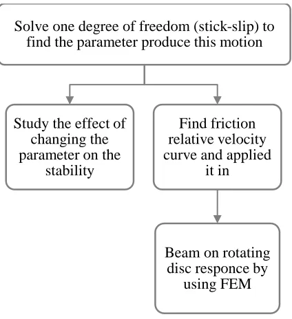
such as mass ratio, damping, and stiffness can make the coupling stiffness between the pad and the rotor to growth and generated stabilize or destabilize system due to the growing of friction layer. H. Hetzler [15] reviews the stability behavior in a vicinity of the steady-state under consideration of a more sophisticated friction model by using mass on moving belt (one degree of freedom system) in an attempted to predict the bifurcation occurrence. This means, that the system may exhibit either an unstable fixed-point or a stable fixed-point. From the previous review the researchers showedthat themass on moving beltis the one most commonly adopted in studies on disc brake squeal whichhas a long and rich history. Although, several models have been, and continue to be, proposed and developed, the classical model for stick-slip. These studied showed that the researcher after developed or build a certain model tried to manipulate the parameters to investigate the system instabilityand match it with the real system condition. However, study stick slip one degree of freedom by one mathematical equation represents three interval of motion instead of using three separated equation for three interval still did not presented. The aim of the paper is to present, solve, predicts the stick slip motion and applied it in finite element software. The paper progress was explained in the next flowchart 1.

Flowchart 1 illustrates the paper progress work

2 STICK-SLIP ONE-DEGREE OF FREEDOM

The aim of this study is to find the friction relative velocity values theoretically and use it to represent the contact between the beam-disc surfaces. Therefore, solving stick-slip for one degree of freedom will help us to find the values which were used later to present stick slip motion in ABAQUS software. Figure 1 shows the system of stick-slip for one degree of freedom: a mass M on a belt, the belt moves at constant speed (v ). The mass is a rigid body having position X (t) at time t. It is subjected to gravity loading Mg, linear spring-loading KX, linear damping force Cd _dt, and a friction relative velocity force. The spring, K is attached parallel to the damper, C and connected to mass, M. The mass bottom is in contact

with a moving band while the mass left side is connected to the spring pivot. The initial length of the spring is Xo with a pivoted point. The band is moved by a constant speed.

Figure 1 Mass at position X (t) on a belt that moves at constant speed

µ is friction coefficient which is a function of the relative velocity (vr=d _dt−v ). It appears that |μ| ≤μ_swhen the mass was at rest on the moving belt (vr=0, stick phase), but when the mass starts sliding |μ| ≥ μ_k (vr≠0, slip phase). However, friction force is time-dependent during stick and velocity-dependent during slip. The friction force is always in the same direction of the belt movement. μ_s, μ_k is the static and kinetic coefficient of friction, respectively. The equation which represents the motion will be:

MẌ +CẊ +KX=F Equation 1

F=μ_sN(Sgn(Ẋ −V ) −σ(Ẋ −V )),

ArdéshirGuran [16]

Equation 2

σ=sigma= friction coefficient versus relative velocity slope

(grade),

V

b _{=belt velocity, N=normal force. By substituting}

equation (2) with equation (1) yield

MẌ +CẊ +KX=μ_sN(Sgn(Ẋ −V ) −σ(Ẋ −V ))

Equation 3

Equation (3) can be rearranged as:

MẌ + (C+ μ_SNσ)Ẋ +KX

= μ_SNSgnN(Ẋ −V ) +σV

Equation 4

The Signum function sgn (vr) or sign (vr) is mathematically described as :

sgn(vr) = {+₋1₁forv_forvr>0

r<0 Equation 5

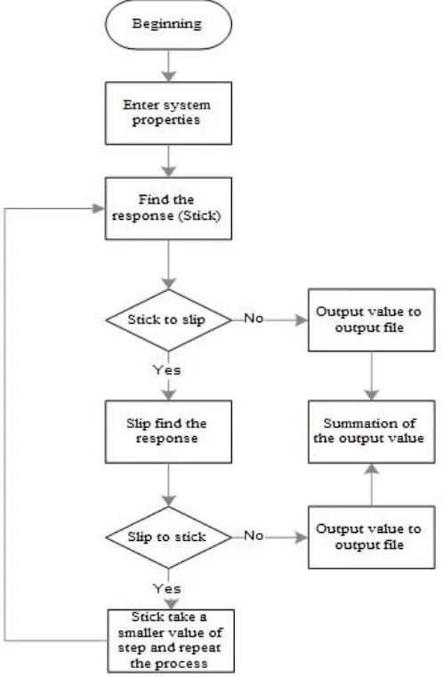
The equation 4 showed that the system is nonlinear due to the change of friction force with the relative velocity. The equation showed also that the friction plays an important value in the damping. The response corresponding to the initial condition can be calculated using fifth-order Runge-Kutta method which was built in MATLAB software as ODE45. The solution method was illustrated in flowchart 2

Solve one degree of freedom (stick-slip) to

find the parameter produce this motion

Study the effect of

changing the

parameter on the

stability

Find friction

relative velocity

curve and applied

it in

Beam on rotating

disc responce by

98

Flowchart 2 stick-slip motion response

3 DYNAMIC ANALYSIS AND DISCUSSION

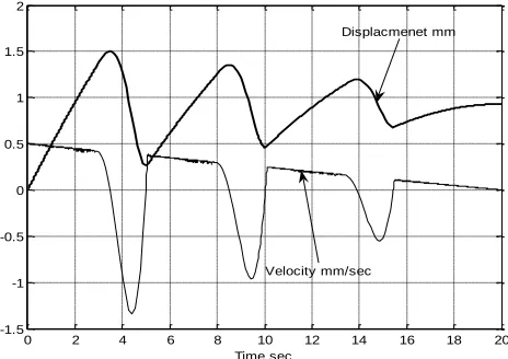
The simulation required a few trials to determine the mass, damping and stiffness values which should be used with the system equation 4 in order to get stick-slip motion same as Ko and Brockely[17] experimental result. The value to achieve stick-slip motion for the system shown in the Figure 2 was; Mass (M) =1 Kg, spring stiffness (K) =5 N/mm, Damping C=1.5 (N. mm)/Sec, Static friction coefficient (μ_S) =0.5, Sigma=0.3, normal load=10, initial displacement=0.0, belt velocity=0.5 mm/sec and mass initial velocity= 0.5 mm/sec. These values were stick-slip achieved was considered as the baseline condition for this analysis. The response depend on the initial condition Ẋ ,Ẍ=0. In the present work, a simple and efficient formula was presented to simulate stick-slip vibrations with signum function. Using signum function in MATLAB software simplifies the method required to solve the stick slip equation. The advantage is that the system can be integrated with any standard ODE-solver available in mathematical packages as MATLAB or ODE-solver of existing software libraries. However, the system can be integrated without need to halt, thus will minimizes the start-up costs. Figure 2 shows the time-varying position X (t) of the mass when there is no external harmonic excitation.

Figure 2 Displacement (mm) and velocity (mm/sec) versus time where, σ=0.5; μ_s=0.5; K=5N/mm; C=1.5N.mm/sec;

N=10N; V =0.5mm/sec

99 of displacement 0.75mm indicated that the mass is at the

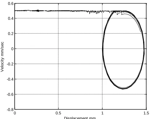
middle of the displacement X (t) trying to return back to the zero position. Thus the potential energy transfer to kinetic energy and lead the mass to be at maximum velocity. However viscous damping and dry friction will drain the energy until a stationary state is achieved with belt velocity equal to mass velocity. Figure 2 was return to plot in a phase plane, figure 3, in order to understand about the velocity-displacement relation.

Figure 3 Phase plot of velocity versus displacement in stick slip motion

The stick appears as horizontal lines in the velocity-displacement phase plot, figure 3, where (d

dt=0). The position (response) of the mass will change linearly with time as long as the mass continues to stick. When the displacement is 1.4mm the sticking stops and the mass start to slip. During the stick the static friction magnitude will increase until it reaches the maximum value of (μ_s).

4 SYSTEM FREQUENCY

The natural frequency is the main cause of the squeal. The squeal appeared at the frequency equal to the system natural frequency. Therefore, it is important to calculate the natural frequency of the system in order to avoid the squeal as in figure 4.

Figure 4 Frequency amplitude plot for one degree offreedom(stick-slip)

The formula 1 was rearrange by assumed that ( ω= √1−ξ ωn) to find the amplitude versus the frequency.

A(ω) = | F

√(K−ω ) +cω | Equation6

F is the friction force. However, the result showed that the system amplitude (peak-zero) increased when the frequency is increased. Then the frequency reach to 0.33Hz the figure showed the maximum amplitude 1.85 mm. The peak indicates that the system reach to its natural frequency. The system amplitude decreased when the frequency increased above 0.33Hz. By comparing the result of figures 4 and 2 it can be appear clearly that the system in the figure 2 vibrates at the natural frequency. To avoid the stick-slip motion the system frequency should be far from its natural frequency. However, increase the velocity of the system can change the system frequency and decrease the stick-slip phenomenon amplitude (peak -zero). The effect of high frequency is to smooth out the discontinuously of the friction. This explains the possibility of eliminating negative slop of the friction and prevents the occurrence of self-excited oscillation.

5 STUDY THEEFFECT OF CHANGING

STICK-SLIP PARAMETERS

The aim of this study was predicting the effect of change the stick-slip parameter on the system stability. The belt velocity in the brake system represents disc speed thus it is important to study the effect of increase the disc velocity on noise. The result in the figure 2 was built on belt linear velocity equal to 0.5 mm/sec. The belt velocity was increased from 0.5 mm/sec to 1 mm/second as in figure 5 in order to study relation between stick-slip and velocity, see figure 3. The simulation was run with same parameters in the section 3.

Figure 5 The system response and velocity, belt velocity is increased to 1 mm/sec.

By increasing the belt velocity the stick period decreased and the motion tends to be close to quasi-harmonic oscillation. The system showed small peak in the velocity curve when the motion changes from slip to stick. This peak indicated the tendency of the mass to continue slipping. Therefore, there is 0 0.1 0.2 0.3 0.4 0.5 0.6 0.7

0.4 0.6 0.8 1 1.2 1.4 1.6 1.8 2

Frequency HZ

A

m

p

li

tu

d

e

m

m

0 2 4 6 8 10 12 14 16 18 20

-4 -3 -2 -1 0 1 2

Time (Sec) Velocity mm/sec

100 still energy in the spring, which might be enough to accelerate

the block above the belt velocity again, and cause another step within the same cycle. It can be observed that the amplitude of the block increased when the belt velocity is increased (peak-peak). By comparing figures 5 and 2, it can be observed that by increasing the belt velocity the slip period increased from 1.4 sec to 2.4 sec. Also by increasing the belt velocity the number of oscillations is increase from 0.25Hz at velocity 0.5mm/second to 0.27Hz at 1mm/sec. This means that increase the disc velocity could make the oscillation increase. The result is similar to that of Ouyang and Mottershead[18] “increase the velocity of the stick slip belt increased the vibration”.Satish Gandhi [19] in his thesis showed the relation between the relative velocity and the amplitude at constant damping value where increase the relative velocity conduct higher amplitude. By compare Satish Gandhi [19] figure with the result of the figure 5, the agreement can be observed where increase the relative velocity lead to increase the amplitude to 1.8 as in figure 4 compare to figure 2. The simulation was run with increase the friction coefficient from 0.5 to 0.8. Figure 6 showed long stick period at the beginning due to increase the static friction coefficient which required higher spring energy to pull it back than figure 2. The number of oscillation was decrease from 0.25Hz at figure 2 to 0.21Hz at figure 6 due to contribute of the friction inside the damping coefficient, see the equation 4. Increase the friction coefficient minimizes the amplitude of oscillation (peak-peak) from 1.5mm at figure 2to 1.25mm at figure 6. This means that the friction is contributed to decrease the amplitude (peak-peak) and the number of oscillation.

Figure 6 The system response with increase the coefficient of friction from 0.5 to 0.8, σ=.5; μ_s=0.8; m=1 Kg; N=10 N; C=1.5

N.mm/sec; v=0.5 mm/sec; K=5N/mm

The period of stick in figure 6 is 4.6 second which it is longer than 2.4 second in figure 2, while the slip period is equal. The amplitude (Peak to zero) in figure 6 (2.5mm) become higher than figure 2 (1.5mm). From entire the discussion it can be said that increase the friction coefficient will make the pad deformation higher but the vibration lower due to increase the friction. The simulation was run again with decrease the damping coefficient result in an increase the number of oscillating (0.33Hz) and decrease the amplitude 0.5mm

(peak-peak), figure 7, than the number of oscillation and the amplitude in figure 2 (0.25Hz, 1.5mm), respectively.

Figure 7 System response due to change the value of damping from 1.5 to 0.1 N. mm/sec, σ=0.5; μ_s=0.5; M=1Kg;

N=10N; V =0.5mm/sec; K=5N/mm

The stick interval is 0.8 second and the slip interval is 2 second, while in the figure 2 was 2.4 second and 1.4 second, respectively. This indicates that decrease the damping the system motion tends to show slip motion only. This mean there was always energy inside the spring, in other words the system cannot reach to the maximum velocity because the dissipation energy was decreased and the potential energy could not be equal to kinetic energy in one point. This could explain why the velocity amplitude in the figure 8 is less than the velocity amplitude in the figure 2. It can be observed that decrease the damping value achieve high amplitude (peak-zero) than figure 2. This result indicated that with low damping high deformation (peak-zero) and number of oscillation appeared in the pad. From the Figure 8 when the damping decreases the system velocity amplitude decreases (peak-peak) if it compare with figure 2, so by decreasing the velocity amplitude (peak-peak) or decreasing the damping coefficient the oscillation amplitude (peak-zero) will decrease but the number of oscillation (peak-peak) will increase. When the relative motion is very small, it is hard to think about the kinematic and static friction as being distinct processes. The result in the figure 7 confirms Meziane and Errico[20] phenomenon of squealing, that the coulomb friction coefficient decreases as velocity increases. Satish Gandhi [19] found the same result as in the figure 7 and 8 by using the condition method to solve stick-slip.

0 2 4 6 8 10 12 14 16 18 20

-2 -1.5 -1 -0.5 0 0.5 1 1.5 2 2.5

Time (Sec) Displacement mm

Velocity mm/sec

0 2 4 6 8 10 12 14 16 18 20

0 0.5 1 1.5

Time (sec)

D

is

p

la

c

m

e

n

e

t

m

101

Figure 8 velocity versus time after change the value of damping from 1.5 N.mm/sec to 0.1 N.mm/sec, sigma=.5; μ_s=0.5; M=1Kg; N=10N; C=0.1N.mm/sec; v =0.5mm/sec;

K=5N/mm

The velocity as a function for displacement (figure 7 with 8) was re-plotted in figure 9. Figure 9 showed that the steady limit cycle occurs when the velocity increased. The cycle showed that there is no stable equilibrium point. Since the plot is a close circle, it means that motion is periodic. This was due to the fact that the dynamic friction coefficient was not very different from the static friction coefficient. Also from the figure 9 the tendency to generate the squeal becomes lower.

Figure 9 Phase plot of velocity versus displacement; σ=0.5;

μ_s=0.5; M=1Kg; N=10N; C=0.1N.mm/sec; v =0.5mm/sec; K=5N/mm

The simulation was done for different value of static friction coefficient in order to see the effect of changing these parameters on the stick-slip motion, Figure 10. Increase the static friction coefficient result in an increase the time for the stick. However, the energy required from the spring to pull the mass back should be increased, according to that the mass

cannot return to the zero position when the static friction is high result in amplitude become high also.

Figure 10 System response for different values of (μ_s); sigma=0.5; M=1Kg; N=10N; C=1.5N.mm/sec; V =0.5mm/sec;

K=5N/mm

It can observed also that with decrease the coefficient of static friction the motion approached quasi-harmonic oscillation this will eliminate the effect of discontinuity but it's not applicable because it is going to reduce the brake efficiency. Figure 10 showed that the number of oscillation increase by decrease the friction coefficient from 0.2Hz at friction coefficient 0.9 to 0.3Hz at friction coefficient 0.2. However, decrease the friction coefficient result in decrease the noise. The simulation was run with different value of contact stiffness while the other parameter is same as section 3. Figure 11 illustrates the relation between the stiffness and the amplitude of oscillation. Increase the stiffness decreased the amplitude (peak-peak) due to increase the kinetic energy of the spring. Figure 11 showed that the number of oscillation increase from 0.097Hz at 2N/mm to 0.416Hz at 12N/mm. However, increase the stiffness mean increase the stick-slip motion and decrease the amplitude (peak-zero). This could be explained by the limit cycle size where the lower stiffness means bigger limit cycle.

Figure 11 Stick-slip for different stiffness value, σ=0.5; μ_s=0.5; M=1Kg; N=10N; C=1.5N/mm/sec; V =0.5mm/sec

0 2 4 6 8 10 12 14 16 18 20

-0.6 -0.4 -0.2 0 0.2 0.4 0.6 Time (sec) v e lo c it y m m /s e c

0 0.5 1 1.5

-0.8 -0.6 -0.4 -0.2 0 0.2 0.4 0.6 Displacement mm V e lo c it y m m /s e c

0 2 4 6 8 10 12 14 16 18 20

-1 -0.5 0 0.5 1 1.5 2 2.5 Time (sec) D is p la c e m e n t m m mus=0.2 mus=0.5 mus=0.9

102 The simulations for different damping coefficient values were

conducted in order to investigate the effect of damping on stick-slip motion, Figure 12.

Figure 12 System response due to different value of damping coefficient; σ=0.5; μ_s=0.5; M=1Kg; N=10N; V =0.5mm/sec;

K=5N/mm

The result showed that decrease the damping from 2N.mm/sec to 0.5N.mm/sec increase the number of oscillation from 0.154Hz to 0.3125Hz. The mass did not return to zero position with low damping because energy dissipation is lower than high damping. In other words, the gradient of the negative slop (relative velocity-friction gradient) increase.

Figure 13 Velocity response due to different value of damping coefficient; σ=0.5; μ_s=0.5; M=1Kg; N=10N; V =0.5mm/sec;

K=5N/mm

Figure 13 showed increase the stick interval by increase the damping result from changing the friction coefficient which it’s already inside the damping matrix. Increase the velocity in figure 13 indicates to increase the dissipation energy which pulls the mass back. The simulation is conducted with different mass value (3, 2, 1) Kg while the other parameters stay constant, figure 14. The result showed that increase the mass has no significant effect on the amplitude (peak-peak). Increase the mass value mean increase the potential energy required to pull the mass back. For M=3Kg the frequency is 0.16Hz while for M=1Kg the frequency is 0.23Hz. This indicates that the number of oscillation increased by decrease

the mass. However, increase the mass can reduce or damp the vibration of the system but the deformation (peak-zero) increase.

Figure 14 System response due difference mass value: Sigma=0.5; μ_s=0.5; M=3Kg; N=30N; C=1.5N.mm/sec;

V =0.5mm/sec; K=5N/mm

6 BELT (DISC) VELOCITY DECLERATION WITH

THE TIME

The velocity deceleration analysis is carried out on one mass which is subjected to friction as a relative velocity function and solved by using Runge-Kutta method (ODE 45). The case of decelerate sliding is important because deceleration is often caused by brake friction. The belt (disc) speed is considered slowly varying linearly with the time until it completely stop. The belt velocity is assumed to decelerate from 0.5mm/sec to zero at 20 second. The result was plotted in the figure 15. The figure showed that the displacement amplitude decrease with the time as the velocity amplitude. The decrease in the velocity amplitude is due to the decrease of the energy that transfers from the supplier (belt) to the mass.

Figure 15 Displacement and velocity versus time, σ=0.5; μ_s=0.5; m=1Kg; N=10N; C=1.5N.mm/sec; V = (0.5-0.025t)

mm/sec; K=5N/mm

0 5 10 15 20 25 30

-1 -0.5 0 0.5 1 1.5 2 Time (Sec) D is pl ac em en t (m m ) C=2 C=1.5 C=0.5

0 5 10 15 20 25 30

-2.5 -2 -1.5 -1 -0.5 0 0.5 1 Time (Sec) V e lo c it y m m /s e c C=2 C=0.5

0 2 4 6 8 10 12 14 16 18 20

0 0.5 1 1.5 2 2.5 3 3.5 4 4.5 Time (Sec) D is p la c e m e n t m m M=3 kg M=2 Kg M=1 Kg

0 2 4 6 8 10 12 14 16 18 20

103 The velocity was plotted versus the displacement in figure 16.

The aim of the study is to understand about the system stability. The result describes the energy pumping from the deceleration belt to the block. Figure 16 showed that the system is stable system, due to the tendency of the system to move to the stable (settle) point. The source of the energy is the driver belt and the energy transmitted to the spring-mass-damper system by the frictional force, and it is not enough to overcome the energy loss through the damper. Thus the friction and the damping combine to act as a mechanism for removing energy from the system. In this case any noise was generated will depend on the initial condition only.

Figure 16 velocity versus displacement

The result which was presented in figure 16 is agreement with Pilipchuk and Tan [3] result. The authors found the effect of decreasing belt velocity on the system by using velocity-displacement phase. The authors system consists of two degree of freedom. They showed that the system velocity-displacement plot tends to the settle point. The authors include in them studied the effect of micro-slip approach beside that the jump phenomenon. This is the reason why the drawing showed a rise in the amplitude before the mass stopped.

7 PLOT FRICTION RELATIVE VELOCITY CURVE

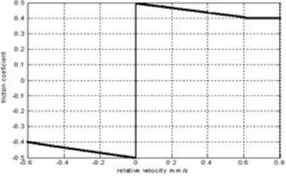
The equation 2 was solved by using ODE45 in order to find the value of friction coefficient versus relative velocity. These values are going to use inside ABAQUS software to represent the contact friction versus slip velocity in beam-disc system.

Figure 17 Friction coefficients versus relative velocity mm/second

Figure 17 showed that at zero relative velocity when the belt and the mass move together (stick), the friction coefficient will increase until it reaches to the maximum value (0.5). The friction coefficient value will decrease when the relative velocity between the mass and the belt generated (slip). When the mass returns to stick the relative velocity will be equal to zero and the friction coefficient may be any arbitrary value between 0.5 and zero. After that the friction coefficient will increase until the slip occurs again. However, by increasing the relative velocity the friction coefficient will decrease until the relative velocity 0.6mm/sec the friction coefficient be a constant value and equal 0.4. The friction behavior is a consequence of the dynamic of the system rather than the interaction properties. At zero sliding velocity, the friction coefficient changed with time. The initial negative slope corresponds to negative damping, and thus causes oscillation to grow up until a balance of dissipated is attained. The results of stick-slip analysis were return to present in flowchart 3.

Flowchart 3 illustrate the stick-slip analysis result

0 0.5 1 1.5

-1.4 -1.2 -1 -0.8 -0.6 -0.4 -0.2 0 0.2 0.4 0.6

Displacement (mm)

V

el

oc

ity

(

m

m

/s

)

M=1, K=10, N=10, mus=0.5, slop=0.3, initial mass velocity=0.5,

enter c and v parameters Beginning Use

ODE45

Increase quasi-harmonic

velocity

when the velocity is decrease linearly from

0.5 to 0

Damping Coefficient

C=1.8

Damping coefficient

C=0.1

Quasi Harmonic Increase

the vibration amplitude

Sticking increase with time until the system stop

104

8 UNDERTANDING THE MECHANISM WHICH

GENERATE FRICTION-INDUCED VIBRATIONS

Eliminating brake noise which is generated during the brake application is an important issue in an improvement of comfort cars. This section presents a study about disc brake groan by using beam and disc. During the braking operation, the friction between the pad and the disc can induce dynamic instability. This instability was mostly unwanted as it generates noise, increase wear, and diminish accuracy. Understanding the mechanisms which generate friction-induced vibrations can help to avoid this unwanted motion (noise). The mechanical interactions in the brake system are very complicated, including a nonlinear contact effects at the friction interface. This section focuses on the groan generated at low frequency due to the nonlinearity of the contact. The earliest research about brake groan suggested that the variation in the friction coefficient with sliding velocity was the cause of self-excited vibration. Not only the difference between the static and dynamic coefficient of friction was the reason for the groan noise at low frequency, but the drop in kinetic friction with increased sliding velocity led to a stick-slip motion and self-excited vibration.

9 STICK-SLIP MOTION, BEAM ON ROTATING

DISC BY USING FE SOFTWARE

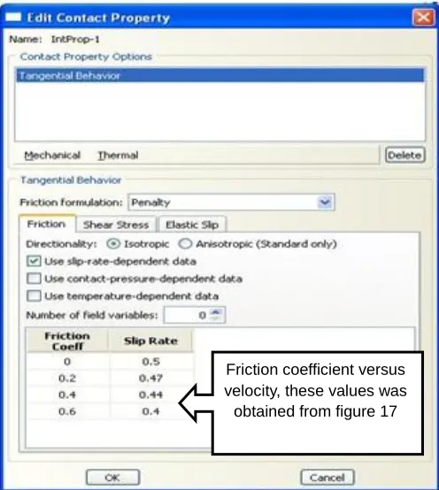
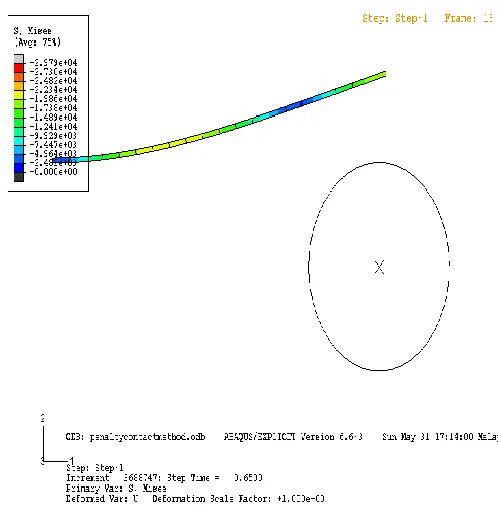
The aim of this study is to find the response of the saw tooth oscillations indicating the occurrence of stick-slip response at low velocity. The following calculation for beam-on-disc was done with kinematic contact method. The left end of the beam was constrained in all the directions but the right end of the beam was not (free end), the boundary condition was illustrated in Figure 19. The friction curve which was found by using MATLAB Software figure 17 was used to represent the surface interaction between the disc and the beam, as in figure 18.

Figure 18 contact property from ABAQUS software

The aim of use ABAQUS software was the ability of this software to change the friction value automatically as the relative velocity value change. ABAQUS understand the maximum value of the friction coefficient as a static value while the lower value as the kinematic friction. ABAQUS change the value of the friction based on the stress generating during the contact. An explicit dynamic finite element was used as a method to simulate the behavior of the system mechanism. The lower beam face contributes as a salve surface for the contact purpose while the master surface was the outer disc diameter. The disc is considered as a master surface because it was a rigid [ABAQUS help]. Because of the disc was a rigid body the reference point required. The reference point represents the point which has six degree of freedom (three transitions and three rotations). The center of the disc was considered as reference point in order to choose it as the point of center rotation. It is possible to model the disc using surface element but in order to reduce the processing time and limitation imposed on the number of elements; a rigid surface is used to represent the disc.

Figure 19 Beam on rigid rotating disc boundary condition The reference point should be fixed in the direction that does not have any rotational velocity; otherwise inertia force should be applied in reverse direction of this motion [ABAQUS help]. The beam material was the same as the pad back-plate material so as to get a better understanding of the pad response to the stick-slip interaction. The measurement was taken at the end point of free beam end.

Figure 20 The stress on beam for final step of the motion Friction coefficient versus

105 The disc was rotated by constant angular velocity 15.2 rev/ min

clockwise which it is equal to the stick-slip linear velocity, this value was conducted form mass-moving belt figure 2. Beam dimension is 100×1 mm and the disc diameter is 25 mm. The beam was deformed body and the rigid disc was undeformed body with the effect the of stick-slip contact. The two bodies were meshed by using a free mesh. The beam and the disc (surface roughness and imperfections) are not taken into account, neither the thermal effect, in this simulation. The response of the free beam end (all the beam elements are constrained kinematically to each other) in the horizontal and vertical direction is found, as seen in Figure 21 and Figure 23. The node atfigure 20 refers to the interaction point which is always in contact, however there is a separation at certain times depend on the friction coefficient and the contact type, as shown in the Figure 22. From Figure 21, the effects of the stick enforce the beam to deflect in the horizontal direction until 0.00029 mm (maximum displacement). At this value the static friction reaches to its maximum value. The beam oscillates about (-0.00015) mm. The beam does not oscillate around its zero equilibrium position due to the effect of static friction which enforces the beam to stick with the disc before the beam return to equilibrium position. When the beam node comes into contact with the disc, the normal stress will increase and causes the node to change from stick to slip. The normal stress at that moment will be bigger than the pressure from the beam. The normal stress decreases after that, so the node returns to the slip rate as before the separation from the disc surface. The separation of the contact surfaces corresponds to local shocks between the two contacting bodies.

Figure 21 Displacement (mm) at beam node1 in horizontal direction versus time (second) with disc rotational velocity

equal 15.2 rev/min

A modal study was performed in order to monitor the movement of the system during the separation as shown in Figure 22.

Figure 22 Beam on disc mode shape, at system frequency 15.2 rev/min

Figure 23 shows the amplitude of oscillation in vertical direction where it is higher than the horizontal direction. By comparing Figures 21 and 23, the peak of the amplitude in each oscillations appeared at same time. This indicates that stick-slip oscillation pushed the beam to move in two directions at the same time but with different amplitude. As a result the effect of the normal force that appeared is higher than the effect of friction force on the beam. The difference in the amplitude in Figure 23 is due to the friction coefficient value. Whenever the mass is stationary, the force of the friction can take any magnitude between zeros to maximum value of static friction.

106 The beam displacement was conducted in figure 21 and 23

while the velocity versus time was conducted in figure 24 and 25. When the system tends to change the friction coefficient from static to kinetic a self-excited vibration can be generated. The velocity will increase as in Figure 24. Increase the velocity did not affect the amplitude of oscillation in horizontal or vertical direction. Increase in the velocity may not always lead to decrease the amplitude of the oscillation and reduce the instability. Friction forces are always parallel to the surface, and the rotation of a disc segment will result in a transverse component of the friction force. These forces that change their direction as the geometry changes are non-conservative and can result in instabilities as mention by Joe et al. 2008. However, the system oscillation velocity start to increase indicated to generate self-excited vibration.

Figure 24 Horizontal velocity at beam node1 with disc rotational velocity 15.2 rev/min

Figure 25 shows that the vertical velocity has increased with the time. The vertical velocity is higher than horizontal velocity due to the difference in beam amplitude. This result indicates that while the system operates in the velocity-range of self-excitation vibration (0-500) kHz, the velocity can increase and it is difficult to remove the self-excited motion. The result in Figure 4-31 indicates that the normal weight only can drive the system into instability. This result is agreed by Ouyang, et al [18] where they found that at very low speeds the in-plane flexibility leads to stick-slip behavior which couples with the transverse motion through the friction force and can raise the insta ilities known in the industry as “ rake groan”.

Figure 25 Vertical velocity versus time of beam at node1

10 BEAM ON ROTATING DISC WITH KINEMATIC

CONTACT METHOD

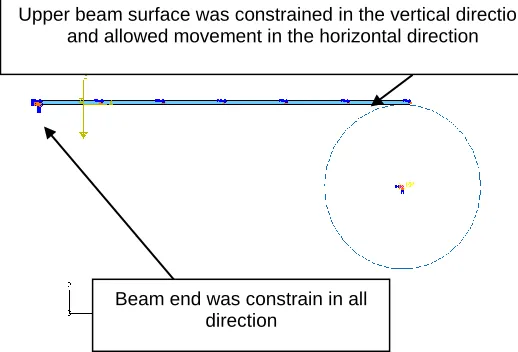
The left end of the beam was constrained in all directions and the upper surface of the beam was constrained from movement in the vertical direction only. The friction curve found by MATLAB Software was used to represent the surface interaction between the disc and the beam. An explicit dynamic finite element was used to simulate the behaviour of the system’s mechanism during frictional contact. Kinematic contact method was applied between the lower surface of the beam and the outer surface of the disc. The aim of this study was to represent the contact between the pad and the disc without surface separation in order to observe the effect of self-excited vibration on the system.

Figure 26 beam on disc boundary condition with rotating velocity 0.5 mm/sec

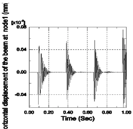
Figure 27 illustrates that the stick-slip motion is the main source to generate the self-excited vibration in low frequency. The horizontal displacement in Figure 27 is higher than the horizontal displacement in Figure 21. This indicates that adding constrain to the system (allow the motion to be in one direction only) led the energy to discharge in other direction. However, the vibration is periodic but the effect of nonlinearity contact made the amplitude to be different between each other.

Beam end was constrain in all direction

107

Figure 27 Horizontal displacement of the beam at node1 The friction force as shown in the Figure 28 kept the mass in equilibrium position (0.0, 0.0) and it was match the beam at the equilibrium position until the friction limit overcome. The force which kept the mass in equilibrium was the value for the static friction force. Once the static value is overcome, the frictional force reverts to the kinetic value. Figure 27 showed that the amplitude of oscillation increased with the time. This increment indicates that the increase in the instability with time as a result of the self-excitation.

Figure 28 Horizontal velocity for the beam at node1 The results in Figures 27 and 28 conclude that, in dry friction the design of the brake components could influence the vibration noise behavior of the brake system because the constrain of the upper surface change the result.

11 BEAM ON DISC WITH PENALTY CONTACT

METHOD

The following simulation for beam on disc was done with penalty contact method where the boundary condition was applied as in the Figure 19. From Figure 29, it observed that the reason for oscillation was the variation of friction coefficient with the relative velocity and made the beam to oscillate at its natural frequency at 0.85 second.

Figure 29 Horizontal displacements versus time at beam node1

108

Figure 30 Vertical displacement at node1 for the beam In this system the disc is a rigid wire, without mass and so without frequency for that the disc frequency does not included in this calculation. The vibration in Figure 30 is due to the beam natural frequency only, as can be observed from the beam deflection shown in Figure 31. This result confirms the experimental result of Yokoi and Mikio[23] (the squeal frequencies of higher modes are equal to the natural frequency of the rod in disc beam system). The normal jump of the slider represents a very specific feature of dry friction, and it can occur in a typical situation: at the very beginning of sliding after the static contact of two surfaces (slip after stick).

Figure 31 Beam on rotating disc deflection with penalty contact method showing the effect of friction on the instability

The total load at the separation time is a summation of the initial normal load (N) and transverse (vertical, mÜ ) motion of

the beam. From Figure 30, it can be said about the car brake system that the pad may not be in complete contact with the disc all the time but there will be a region of pad contact that might move during the braking process due to the dynamics of the brake system. The system is described to be unstable when the vertical motion of the system beam becomes so violent that the total normal force become negative or several times larger than the initial normal force (N) and so the motion tends to diverge as also illustrated in Figure 31. Mezian and Errico[21] agreed that the separation is the cause of instability; this unstable state is characterized by the stick-slip-separation wave. The authors also showed that the instabilities described the shock phenomenon at the contact interface. The velocity of the horizontal direction in Figure 32 has increased three times than Figure 29, for same disc speed. This indicates that increase the instability due to the increase in the contact stiffness causes the increase in the beam horizontal velocity. Non-linearity provided by the stick–slip phenomenon includes not only variation in the coefficient of friction but also the variation in contact stiffness due to formation of friction layers on the interface. However, this non-linearity and the increase in the contact stiffness cause the velocity increment. The growth of friction layers affects the contact stiffness considerably, thereby affecting stability of the system. It was observed that with the increase in coupling stiffness, defined by the stiffness of the friction layer, the instability in the beam (pad) increases. This result is in agreement with Paliwal et al [14] and Oden [22] results.

109

Figure 33 Illustrated is the relation between the vertical velocity and the time

The velocity in Figure 33 is higher than the velocity of Figure 25, approximately five times. The velocity did not increase sinusoidal with the time as in Figure 33. Increase in the contact stiffness cause an increase in the velocities and displacements in all direction of the motion. When instability occurs, the contact surface of the pad can stick, slip or separate locally from the surface of the disc. The separation of the contact generated impact forces that cause the groan to occur (at low velocity), Ibrahim [24] obtained the same result but the amplitude was lower, the difference being in the velocity value.

12 THE EFFECTS OF CONTACT ANGLE ON THE

VIBRATION AMPLITUDE

The following calculation for beam on rotating disc has been done with kinematic contact method where the boundary condition is illustrated in Figure 34. The left end of the beam is restrained in all directions while the entire beam has free motion.

Figure 34 Beam on rotating disc with Kinematic contact method, the angel of the contact is 30 degrees

The angle of contact was set to 30 degrees. The force of the contact between the disc and the beam was a beam weight only. The disc rotation velocity is 15.2 revolutions per minute (clockwise), same as horizontal beam position. The beam is a

deformed body while the disc is rigid undeformed body. The aim is to study the effect of the pad contact angle on the groan with stick-slip motion. Beam dimension is 100×1 mm and the disc diameter is 25 mm. The motion variation of the system depends on the structural configuration of the friction system that can cause changes in the normal and friction force. Negative damping acts as an energy input/accumulating mechanism to a self-excited system.

110

Figure 36 Horizontal velocity for the beam at node1

13 CONCLUSIONS

The coefficient of friction plays an important role in system stability. It was proven that the brake noise was due to the variation of the spring stiffness and the damping coefficient. This means that the reduction or generation of brake noise can also be achieved by changing these two parameters. However, the motion is governed by static friction force in the stick phase and a velocity dependent kinetic friction in the slip phase. Stick is due to the high static friction between the surfaces, and slip is due to the lower kinetic friction during the slip itself. As the sliding speed increases there is a critical speed when stick slip vibration disappear. Increase the friction coefficient damped the oscillation while decrease the damping value increase the pad deformation and decrease the stick-slip oscillation (noise). Increase the mass value damped the oscillation or stick-slip motion. Increase the stiffness led to increase the stick-slip oscillation. Decrease the friction coefficient decrease the stick-slip oscillation but it reduce the brake efficiency at the same time. The boundary condition plays an important role in generating stick-slip motion. It was found that by increasing the mass value, the sticking interval gets longer and quasi-harmonic. The transfer from stick to slip was the reason to increase the stress between the surfaces result in a shock or spark made the two surfaces separate. More constrain for the pad result in an increase the oscillation in all other direction which it does not constrain.As affirmation above the result prove that the solution method of stick slip is correct and the application result is match with other people works

REFRENCES

[1]. Martins, J.A.C., Oden, J.T., Simoes, F.M.F., 1990. A study of static and kinetic friction. Int. J. Eng. Sci. 28, 29–92.

[2]. F.P. Bowden, L. Leben, The nature of sliding and analysis of friction, Proc. R. Soc. London, Ser. A 169 (1939) 371–391.

[3]. Pilipchuk and Tan, 2004. Creep-slip capture as a possible source of squeal during decerated sliding, Nonlinear Dynamics 35.

[4]. Shaw, S.W.: On dynamic response of a system with dry friction. J. Sound Vib. 108(2), 305–325 (1986).

[5]. K. Popp, P. Stelter, Nonlinear oscillations of structures induced by dry friction, in: Proceedings of IUTAM Symposium on Nonlinear Dynamics in Engineering Systems, Stuttgart, 1989.

[6]. S. Nagarajaiah, A.M. Reinhorn, M.C. Constatinou, Torional coupling in sliding base-isolated structure, ASCE J. Struct. Engrg. 119 (1) (1993) 130–149.

[7]. Den Hartog, J.P.: Forced vibrations with combined Coulomb and viscous friction. Trans. ASME APM-53-9, 107–115 (1931).

[8]. Brecht, J., Hoffrichter, W., Dohle, A.: Mechanisms of brake creep-groan. SAE Technical Paper 973026 (1997)

[9]. Cao, Q., Ouyang, H., Mottershead, J.E., Brookfield, D.J., James, S.: Stick-slip vibration in a disc brake system. In: Proceedings of the Braking 2002 – From the Driver to the Road, Leeds, UK, pp. 101–109, (2002).

[10]. Abdelhamid, M.K.: Creep-groan of disc brakes. SAE Technical Paper 951282, Proceedings of the 1995 NoiseVibration Conference, Traverse City, MI (1995).

[11]. Q. Feng, A discrete model of a stochastic friction system, Comput. Methods Appl. Mech. Engrg. 192 (2003) 2339–2354.

[12]. P. Filip, Friction and wear of polymer matrix composite materials for automotive braking industry, in: Braking 2002, IMechE, International Conference of Automobile Braking, Leeds, UK, 2002, pp. 341–354.

[13]. M. North, A mechanism of disc brake squeal, in: 14th FISITA Congress, no. 9 in 1, 1972.

[14]. Manish Paliwa et al. Noise and vibration analysis of a disc–brake system using a stick–slip friction model involving coupling stiffness. Journal of Sound and Vibration 282 (2005) 1273–1284.

[15]. H. Hetzler *, D. Schwarzer, W. Seemann. “Analytical investigation of steady-state stability and Hopf-bifurcations occurring in sliding friction oscillators with application to low-frequency disc rake noise”. Communications in Nonlinear Science and Numerical Simulation 12 (2007) 83–99

[16]. A Book: ArdéshirGuran et al. 2001. Dynamics with friction: modelling, analysis and experiment, part II. World scientific publishing Co. Pte. Ltd.

111 [18]. Ouyang, H., Mottershead, J.E., Cartmell, M.P. and

Friswell, M.I. 1998. Friction-induced parametric resonances in discs: effect of a negative friction-velocity relationship. Journal of Sound Vibration, Vol. 209, No. 2, pp.251–264.

[19]. A Thesis: Satish Gandhi, 1998. Study of Friction Effects on System Dynamics Using Low-Order Lumped-Parameter Models, M.S. thesis, Panjab University, India.

[20]. Meziane and Errico, 2006. Instability genereated by friction in a pad-disc system during the breaking. Journal of sound and vibration.

[21]. Mcmillan, A., J. 1997. A non-liner friction model for self-excited vibration. Journal of Sound and Vibration. 205(3), 323-335

[22]. Oden, Becker and Tworzydlo, 1992. Numerical modeling of friction-induced vibration and dynamic insta ilities.‖ Friction induced vi ration, chatter, squeal and chaos ASME 1992.

[23]. M. Yokoi and M. Nakai, 1980. A fundamental study on frictional noise, 2nd report: The generating mechanism of squeal noise of higher modes. Bull. JSME 23, No. 186, 2118 –2124.process.

[24]. Ibrahim, R. A., 2002. Friction-Induced Noise and Related Problems in Automotive Brakes. Recent Research Developments in Sound & Vibration, 99-131, Transworld Research Network, Kerala, India.