e-ISSN: 2278-067X, p-ISSN: 2278-800X, www.ijerd.com
Volume 14, Issue 2 (February Ver. I 2018), PP.16-20
Analysis of Improved DV-Distance Algorithm for Distributed
Localization in Wsns.
1
Sudha H. Thimmaiah and
2G.Mahadevan
1
Research Scholar, Dept. of ECE, PRIST University, Thanjavur, Tamil Nadu, India.
2Principal, Dept. of CSE, Annai College of Engineering, Kumbakonam, Tamil Nadu, India.
Corresponding Author:
[email protected]
ABSTRACT: Node localization is one of the important supporting technologies in Wireless Sensor Networks. The process of node localization depends on the accuracy of determining the position of the nodes in the required environment. Most of the applications of WSNs require the knowledge of the location of the sensors. The main task of a wireless sensor node is to sense and collect data from a certain domain, process the data and transmit the same to the anchor node. In this paper, both the DV-distance localization algorithm and the improved version of the same is analysed for localization errors. In the DV-distance algorithm, the cumulative distance is obtained by the use of distance vector routing whereas, in the improved DV-distance algorithm hops are introduced between anchor and unknown nodes to determine the distance. Simulation results show that, localization accuracy of the improved algorithm is better than the DV-distance algorithm.
KEYWORDS: Algorithm, DV-distance, Localization, Wireless Sensor Networks,
--- --- Date of Submission: 10 -02-2018 Date of Acceptance: 26-02 2018 ---
---I.
Introduction
Wireless Sensor Networks is one of the recent networking fields which have gained significance in several key research areas. A wireless sensor network is composed of a large number of sensor nodes densely deployed in the sensor network domain. The sensor nodes in the network domain must be able to sense and collect data, process the data and transmit the data to the anchor or beacon node in most applications. Wireless Sensor Networks have wide application prospects including search and rescue, disaster relief, target tracking and smart environments. Hence, location awareness is a key factor for the success of the applications. According to the different information needed in the process of node localization, positioning algorithm can be classified into two kinds: Range-based and Range-free [1]. Dragos Niculescu in Rutgers University, who depended on the distance vector routing and GPS principles, proposed a series of distributed positioning algorithms which is well known as Ad Hoc Positioning System – APS [2]. It includes six algorithms: DV-Hop, DV-Distance, Euclidean, DV-Coordinate, DV-Bearing and DV-Radial. Amongst these, the most popular and successful algorithm is the DV-Hop and DV-Distance localization algorithms.
II.
Review Of DV-Distance Algorithm
The DV-Distance is similar to the DV-Hop, but with the difference that distance between neighbouring nodes is measured using Received Signal Strength Indication (RSSI) and the data is propagated in meters rather than hops. The cumulative distance is then calculated by using the method similar to the distance vector routing. DV-Hop localization approach is composed of three phases:
In the first phase, a typical distance vector routing mechanism is employed. Beacons flood their location information throughout the network with the initial hop-count of zero. Each node that relays the message increases the hop-count by one. After the flooding procedure, every node can obtain the minimum hop count to each beacon.
In the second phase, each beacon, after obtaining the position and hop-count information to all other beacons, estimates the average distance per hop. For example, beacon I calculated the average distance per hop, called the hop size HS, using the formula,
HSi = ∑√ ( xi – xj)2 + (yi – yj)2 / ∑ hj
Where ( xi , yi ) and ( xj, yj ) are the coordinates of beacons i and j respectively, and hj is the hop-count value
In the last phase, before conducting the self-localization, each sensor estimates the distance to each beacon based on its hop-count and the hop-size to this beacon. For example, sensor k, can get the distance dkj, the distance from sensor k to beacon j by using, dkj = hj X HSj. After obtaining all the distance information, each sensor conducts the triangulation or maximum likelihood estimation to estimate its own location. This localization algorithm will only work well in isotropic networks [3].
The DV-Distance localization algorithm in6 uses the method of distance vector routing to obtain the cumulative distance. When the unknown nodes get three or more cumulative distances from anchors, then the trilateration method is used to calculate the localization. The DV-distance localization algorithm can be divided into three steps [7].
In the first step, each anchor node broadcasts a beacon to be flooded through the network containing the anchors localization with node ID and RSSI. Each receiving node calculates the distance between its adjacent nodes based on the RSSI theoretical model. Then they will count the cumulative distance or the polyline-distance (disi.j) from themselves to anchors that they can receive by cumulating the
polyline-distance between hop to hop.
In the second step, once an anchor node i gets the polyline-distance to another anchor node j, it calculates an correction ratio (cori.j) of polyline-distance (disi.j) to Straight-line (Disi.j) between the two anchors i,j based
on (1), which is then flooded to the entire network as the network correction. When an unknown node k accepts the information from one anchor node j, it uses the polyline-distance (disi.j) from anchor nodes to
compute the amended distance (DisCorrk.j) between itself and the anchor node as the following Equation (2)
In the last step, when the unknown nodes get three or more distances from anchors, and then unknown nodes calculate their localization by trilateration or maximum likelihood estimation.
DV-Distance replaces the hops in DV-Hop with the polyline-distance which is calculated based on the RSSI model. Thus, it reduces the error due to consider that the rough distance of each hop is equal. The implementation of the algorithm is easy, but, with the ranging error increasing, the localization error also sharply increases [4]. The DV-Distance localization algorithm for localization is used when all the nodes in the network have the ranging capability.
III.
Review Of Improved DV-Distance Algorithm
The improved DV-Distance algorithm takes into account most of the jumping segment of the unknown node and anchors from its nearest anchor node to other anchors is overlap. So, when the unknown node selects the distance correction parameter (Correction), the unknown node selects the original distance correction parameter which has been broadcasted to the networks, if the anchor is the closest node to this unknown node. Otherwise, the unknown nodes use corrections of its nearest anchor node to the other anchor nodes, instead of the unknown node to the other anchor nodes. The proposed algorithm, only requests the anchors have the capability to save the Corrections [5].
In the first step, the proposed algorithm is similar with DV-Distance. The difference is that it uses the method similar with the distance vector routing to get the cumulative distance and the cumulative hops.
In the second step, once an anchor gets the polyline distance to other anchors, it calculates the correction with the following Equation (3)
Where, disi.jis the polyline-distance of anchor i and j, Disi.jis the beeline-distance of anchor i and j, Hopi.jis the
Then, it saves the Correction and the anchor ID to its established list in the memory, and then broadcasts the Correction which is the correction parameter form the nearest anchor node to the network, using controlled flooding. This scheme could ensure that the most nodes receive the Correction from beacon node that has the least distance. When the unknown node gets the Correction from an anchor node, and then it saves this Correction as the correction parameter between this unknown node and its nearest anchor node. Then, the unknown node returns its node ID and other anchor ID which has been saved in the Memory list of this unknown node, and then the answer anchor node sends the corrections which the unknown node need back to the unknown node. The unknown node gets the corrections to all the anchors that its ID has been saved. Then, it calculates the corrected distance with the following equation (4)
(4)
Where, disk.i is the polyline-distance of anchor i and unknown node k, Correctionk.i is the correction of anchor i
and unknown node j, DisCorrk.i is the cumulative-distance of anchor i and unknown node.
In the last step, implementing the trilateration positioning gets the coordinates of all unknown nodes.
IV.
Methodology / Implementation
Wireless Sensor Networks consists of three kinds of nodes – target node, unknown node and anchor node. The number of hops and polyline distance of each unknown node should be found out with respect to anchor nodes, the number of hops and polyline distance between target node and anchor node should be determined. The correction is done for all the parameters using improved DV-Distance method and trilateration to get the localization co-ordinates [6, 7]. MATLAB 9.0 is used to simulate the improved DV-Distance algorithm. The proposed algorithm is divided into three modules: (1) WSN Deployment (2) Improved DV-Distance method (3) Trilateration
(1) WSN Deployment
In this module, the specification of anchor nodes and unknown nodes is given as the input, the co-ordinates of each node are generated randomly and the communication range between one node and the other is defined to get the set of nodes within the communication range to form the connected WSN and represented in figures 1 and 2.
Input: The number of anchor and unknown nodes Output: Connected WSN
Random Distribution of Sensor Nodes
Fig 2. The Sensor nodes communicating within the sensing range.
(2) Improved DV-Distance method:
Improved DV-Distance algorithm is applied to the connected WSN and represented in figure 3. Input: Connected network, polyline distance, number of hops, beeline distance.
Output: the corrected distance of each unknown nodes to the nearest anchor nodes.
(3) Trilateration:
The trilateration method is applied to obtain the estimated position of unknown nodes as shown in figure 3. Input: the corrected distance of each unknown nodes to the nearest anchor nodes.
Output: The estimated localization co-ordinates of unknown nodes. Localization of all unknown nodes
Fig 3. Plot between each node and the estimated position of x-coordinate and y-coordinate values after the improved DV-Distance and trilateration method is applied for the estimation position of unknown nodes.
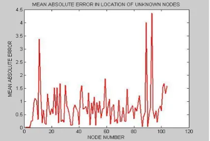
Performance of localization
Figure 4 represents a plot of node numbers on the X – axis and the mean absolute error in the Y – axis and hence the performance of localization.
V.
Results And Discussion
The simulation results showed the deployment of random nodes, their connections within the communicating range, the estimation of localization with improved DV-Distance algorithm and trilateration method [8,9]. The obtained localization of unknown nodes shows very little error compared to the exact localization values. The mean absolute error in the localization of unknown nodes is almost an average throughout with only a few peaks at some nodes [10, 11].
VI.
Conclusion
Hence, the estimation of the location accuracy is improved and thus verified. Further improvement in the location accuracy can be increased with more computing complexity and storage capacity of anchor nodes.
References
[1]. Shu Wang, Yujie Yan, Fuping Hu and Xiaoxu Qu. “Wireless Sensor Networks Theory and Applications”. Beijing University of Aeronautics and Astronautics Press, 141-164, 2007.
[2]. Nicolescu, D. and Nath, B. “DV based positioning in ad hoc networks”. Journal of Telecommunication Systems, 22(1/4): 267-280, 2003.
[3]. Sun Limin, Li jianzhong and Chen Yu. “Wireless Sensor Networks [M]”. Tsinghua University Press, 148-154, 2005.
[4]. Wang Fubao, Shi Long and Ren Fengyuan. “Self-localization systems and algorithms for wireless sensor networks”. Ruan Jian Xue Bao / Journal of Software, 16(5): 857-868, 2005.
[5]. Dianhong Wang, Hongdong Jia, Fenxiong Chen, Fei Wen and Xingwen Liu. “An Improved DV-Distance Localization Algorithm for Wireless Sensor Networks”. Proceedings of the 2nd IEEE International Conference on Advanced Computer Control, ISBN-978-1-4244-5848-6/10/ 472-476, 2010.
[6]. Nicolescu, D. and Nath, B. “Ad-Hoc positioning systems (APS)”. Proceedings of the 2001 IEEE Global Communications Conference (GCC „01).New York, USA, 2926-2931, 2001.
[7]. Yang Feng, Shi Haoshan and Zhu Lingbo. “An Intelligent Localization System Based on RSSI Ranging Technique for WSN”. Journal of Transducer Technology, 21(1): 135-140, 2008.
[8]. Zhang Donghong, Li Kejie and WU Deqiong. “An Improved DV-Distance Self-localization Algorithm”. Journal of Projectiles, Rockets, Missiles and Guidance, 3: 275-277, 2008.
[9]. Liu Lin and Fan Pingzhi. “An Improved positioning algorithm with reduced node location error for wireless sensor network”. Journal of Signal and System, 12(2): 1-4, 2007.
[10]. Xiao Chen and Benliang Zhang. “Improved DV-Hop Node Localization Algorithm in Wireless Sensor Networks”. International Journal of Distributed Sensor Networks, Article ID 213980. doi:10.1155/2012/213980, 2012.
[11]. Shi, L. and Wanf, F.B. “Self-localization systems and algorithms for wireless sensor networks”. Journal of Software, 16(5): 857-868, 2005.