75
ARTIFICIAL NEURAL NETWORKS FOR COMPRESSION OF
DIGITAL IMAGES: A REVIEW
1VENKATA RAMA PRASAD VADDELLA, 2KURUPATI RAMA
1Professor of IT, Sree Vidyanikethan Engineering College, Tirupati, India
2Head of Electronics and Communication Engineering,
Government Polytechnic, Chandragiri, Near TIirupati, India
E-mail: [email protected]
ABSTRACT
Digital images require large amounts of memory for storage. Thus, the transmission of an image from one computer to another can be very time consuming. By using data compression techniques, it is possible to remove some of the redundant information contained in images, requiring less storage space and less time to transmit. Artificial Neural networks can be used for the purpose of image compression. Successful applications of neural networks to vector quantization have now become well established, and other aspects of neural networks for image compression are stepping up to play significant roles in assisting the traditional compression techniques. This paper discusses various neural network architectures for image compression. Among the architectures presented are the Kohonen self-organized maps (KSOM), Hierarchical Self-organized maps (HSOM), the Back-Propagation networks (BPN), Modular Neural networks (MNN), Wavelet neural Networks, Fractal Neural Networks, Predictive coding Neural Networks and Cellular Neural Networks (CNN). The architecture of these networks, and their performance issues are compared with those of the conventional compression techniques.
Keywords: Neural Networks, Image compression,Vector quantization
1. INTRODUCTION
Digital image compression is a key technology in the field of communications and multimedia applications. A large number of techniques have been developed [13] to make the storage and transmission of images economical. These methods can be lossy or lossless. Over the last decade, numerous attempts have been made to apply artificial neural networks (ANNs) for image compression [9, 34, and 35]. The Kohonen self-organizing maps (SOM) [16],[1], Hierarchical SOMs (HSOMs)[3], Back-propagation networks (BPNs) [15], Modular Neural networks (MNNs) [32], and Cellular Neural Networks[30 ], among others have been proposed in the literature. Research on neural networks for image compression is still making steady advances. In this paper, we discuss the various neural network architectures for compression of still images. A comparison on the performance of these networks is made with those of the conventional algorithms for image compression. This paper consists of five
sections. Section 2 discusses the SOMs and HSOMs for image compression using VQ. Section 3 describes the various back propagation neural networks for image compression. In Section 4 modular neural networks are presented. Wavelet and Fractal neural networks are discussed in section 5. Cellular neural networks are described in section 6. Finally, Section 7 gives the conclusions and the scope for future research work in this area.
2. SELF-ORGANIZING MAPS (SOMS)
2.1 Kohonen’s Self-organizing maps (KSOM)
76 (code words) in this space is selected in order to approximate as much as possible, the distribution of initial vectors extracted form the image. Third, each vector from the original image is replaced by its nearest codeword. Finally, during transmission, the index of the codeword is transmitted. Compression is achieved if the number of bits used to transmit the index (log2 l) is less than the
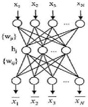
number of initial bits of the block (τ x τ x m); where m is the number of bits per pixel. Kohonen’s self-organized feature map (KSOM) is a reliable and efficient method to achieve VQ for image compression. The basic structure of KSOM is shown in Figure 1. Compression ratios of 10:1 to 100:1 have been reported using the SOM [25]. The search complexity is of order O (N).
Figure 1 SOM Neural Network for Vector Quantization
22 Hierarchical Self-organizing maps (HSOM)
HSOM is an extension of the conventional SOM. A tree-structure is defined, where each node is a SOM, trained with one determined data set. The map in level-1 is trained with the full set of data, and in accordance with the quantization of each neuron, the map children are trained with subgroups of this. Fig.2 illustrates the configuration of the HSOM. The trained HSOM is executed sequentially, i.e., from the highest to the lowest level of the tree. The complexity of
search is reduced to O(log N) in the HSOM.
Figure 2 Configuration of Hierarchical SOM
3. BACK-PROPAGATION NETWORKS
3.1. Basic back-propagation neural network
Back-propagation neural networks are directly applied to image compression [9, 24]. The neural network structure is shown in Figure 3. Three layers, one input layer, one output layer and one hidden layer are designed. The input layer and output layer are fully connected to the hidden layer. Compression is achieved by designing the value of K, the number of neurons at the hidden layer less than that of neurons at both input and the output layers. The input image is split up into blocks or vectors of 8x8, 4x4 or 16x16 pixels. When the input vector is referred to as N -dimensional which is equal to the number of pixels included in each block, all the coupling weights connected to each neuron at the hidden layer can be represented by {wji , j=1, 2,…, K and i=1, 2,…,
N}, which can also be described by a matrix of order KxN. From the hidden layer to the output layer, the connections can be represented by {w’ij :
1≤ i ≤N, 1 ≤j≤ K} which is another weight matrix of order NxK. Image compression is achieved by training the network in such a way that the coupling weights, {wji }, scale the input vector of
N-dimension into a narrow channel of K -dimension (K<N) at the hidden layer and produce optimum output value which makes the quadratic error between input and output minimum.
Figure 3 back propagation Neural Network
3.2. Hierarchical back-propagation neural network
77 by adding two more hidden layers into the existing network as proposed in [24]. The Hierarchical neural network structure is illustrated in Fig. 4 in which the three hidden layers are termed as the combiner layer, the compressor layer and the de-combiner layer. The idea is to exploit correlation between pixels by inner hidden layer and to exploit correlation between blocks of pixels by outer hidden layers
Figure 4. Hierarchical Neural Network Structure
From the input layer to the combiner layer and from the de-combiner layer to the output layer, local connections are designed which have the same effect as M fully connected neural sub-networks. As seen in Fig. 4, all three hidden layers are fully connected. The basic idea is to divide an input image into M disjoint sub-scenes and each sub-scene is further partitioned into T pixel blocks of size pxp. For a standard image of 512x512, as proposed [24], it can be divided into 8 sub-scenes and each sub-scene has 512 pixel blocks of size 8x8. Accordingly, the proposed neural network structure is designed to have the following parameters:
The total number of neurons at the input layer is
Mxp2 = 8x64 =512. Total number of neurons at the
combiner layer is MxNh =8x8=64. Total number of neurons at the compressor layer is Q = 8. The total number of neurons for the de-combiner layer and the output layer is the same as that of the combiner layer and the input layer, respectively. A so-called nested training algorithm (NTA) is proposed to reduce the overall neural network training time, which comprises the following steps:
Step1: Outer loop neural network (OLNN) training.
Step2: Inner loop neural network (ILNN) training.
Step3: Reconstruction of the overall neural networks.
After training is completed, the neural network is ready for image compression in which half of the network acts as an encoder and the other half as a decoder. The neuron weights are maintained the same throughout the compression process.
3.3. Adaptive back-propagation neural network
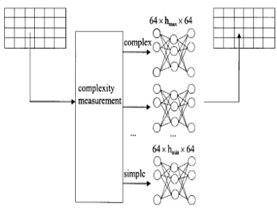
Further to the basic narrow channel back-propagation image compression neural network, a number of adaptive schemes are proposed [4, 9] based on the principle that different neural networks are used to compress image blocks with different complexity. The general structure for the adaptive schemes are shown in Figure-4 in which a group of neural networks with increasing number of hidden neurons, (hmin, hmax), is designed. The
basic idea is to classify the input image blocks into a few sub-sets with different features according to their complexity measurement. A fine tuned neural network then compresses each sub-set. Four schemes are proposed [9] to train the neural networks which are classified as parallel training, serial training, activity-based training and activity and direction based training schemes.
3.4. Performance Considerations
Considering the different settings for the experiments reported in various sources [9],[23],[24], it is difficult to make a comparison among all the algorithms presented in this section.
78 To make the best use of all the experimental results available, we take Lena as the standard image sample and summarize the related experiments for all the algorithms as illustrated in Table1 which are grouped into basic back propagation, hierarchical back propagation and adaptive back propagation.
Table 1 Basic Back Propagation on Lena (256x256)
Table 2 Hierarchical Back Propagation on Lena (512x512)
Table 3 Adaptive Back Propagation on Lena (256x256)
4. MODULAR NEURAL NETWORKS
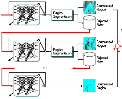
Though a single neural network can compress the average characteristic for the image data, it is difficult to compress both the edge and flat regions with the same precision. For this, Rahim et al. have proposed the compression method using two neural networks [26]. One of the neural networks is used for the compression of the original image and the other is used for the compression of the residual image. However, it is effective to compress for each region, which is divided in to the edge and flat regions. A modular structured neural network consisting of multiple neural networks with different block sizes (the number of input units) for region segmentation has been proposed by Watanbe and Mori [32]. By the region segmentation, each neural network is
assigned to each region such as the edge or the flat region.
From simulation results, it is shown that the proposed method yields a better compression compared with the conventional compression technique using a single neural network.
5. NEURAL NETWORK DEVELOPMENT OF EXISTING TECHNOLOGY
In this section, we show that the existing conventional image compression technology can be developed right into various learning algorithms to build up neural networks for image compression. This will be a significant development in the sense that various existing image compression algorithms can actually be implemented by one neural network architecture empowered with different learning algorithms. Hence, the powerful parallel computing and learning capability with neural networks can be fully exploited to build up a universal test bed where various compression algorithms can be evaluated and assessed. Three conventional techniques are covered in this section, which include wavelet transforms, fractals and predictive coding.
5. 1. Wavelet neural networks
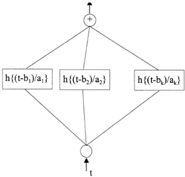
Based on wavelet transforms, a number of neural networks are designed for image processing and representation [8],[20]. When a signal s(t) is approximated by daughters of a mother wavelet
h(t), for instance, a neural network structure can be established as shown in Fig. 7 [8],[20]. Here,
Figure 6. Modular Neural Network
Dimension
N Training schemes PSNR (dB) Bit rate (bpp) 64
Non-Linear 25.06 0.75 64 Linear 26.17 0.75
Dimension,
N Training schemes PSNR (dB) Bit rate (bpp) 4 Linear 14.40 1 64 Linear 19.75 1 64 Linear 25.67 1
Dimension, N
Training schemes
PSNR (dB)
Bit rate (bpp) 64 Activity
based Linear
27.73 0.68
64 Activity and
direction
79 step1 computes a search direction [s] at iteration i. Step2 computes the new weight vector using a variable step-size α. By simply choosing the step-size α, as the learning rate, the above two steps can be constructed as a learning algorithm for the wavelet neural network in Fig.7. Experiments reported [19] on a number of image samples support the wavelet neural network by finding out
that Daubechie’s wavelet produces a satisfactory compression with the smallest errors. Haar’s wavelet produces the best results on sharp edges and low-noise smooth areas.
Figure 7 Structure of Wavelet Neural Network
5. 2. Fractal neural networks
Fractal configured neural networks [22,17], based on iterated function system (IFS) codes [11], represent another example along the direction of developing existing image compression technology into neural networks. Its conventional counterpart involves representing images by fractals and each fractal is then represented by so-called IFS, which consists of a group of affined transformations. To generate images from IFS, random iteration algorithm is the most typical technique associated with fractal based image decompression [11]. Hence, fractal based image compression features higher speed in decompression and lower speed in compression. By establishing one neuron per pixel, two traditional algorithms of generating images using IFSs are formulated into neural networks in which all the neurons are organized as a topology with two dimensions [17]. The network structure is illustrated in Fig. 8 in which wij,i’j’ is the coupling
weight between (ij)th neuron to (i’j’)th one, and sij
is the state output of the neuron at position (i,j). The training algorithm is directly obtained from the random iteration algorithm in which the coupling weights are used to interpret the self-similarity between pixels [64]. In common with most neural networks, the majority of the work operated in the neural network is to compute and optimize the coupling weights, wij,i’j’. Once these
have been calculated, the required image can typically be generated in a small number of iterations. Hence, the neural network implementation of the IFS based image coding system could lead to massively parallel implementation on a dedicated hardware for generating IFS fractals. Although the essential algorithm stays the same as its conventional algorithm, solutions could be provided by neural networks for the computing intensive problems, which are currently under intensive investigation in the conventional fractal based image compression research area.
Figure 8 Fractal Neural network
5. 3. Predictive coding neural networks
80 (linear predictive coding), PCM (pulse code modulation), DPCM (delta PCM) or their modified variations. Non-linear predictive coding, however, is very limited due to the difficulties involved in optimizing the coefficients extraction to obtain the best possible predictive values. Under this circumstance, a neural network provides a very promising approach in optimizing non-linear predictive coding [9, 21].
Based on a linear AR model, a multilayer perceptron neural network can be constructed to achieve the design of its corresponding non-linear predictor as shown in Fig. 9. For the pixel
Figure. 9 Predictive Neural Network
Xn which is to be predicted, its N neighboring pixels obtained from its predictive pattern are arranged into a one dimensional input vector
X={Xn-1, Xn-2,…,Xn-N} for the neural network. A
hidden layer is designed to carry out back propagation learning for training the neural network. Predictive performance with neural networks is claimed to outperform the conventional optimum linear predictors by about 4.17 and 3.74 dB for two test images [21]. Further research, especially for non-linear networks, is encouraged by the reported results to optimize their learning rules for prediction of those images whose contents are subject to abrupt statistical changes.
6. CELLULAR NEURAL NETWORKS
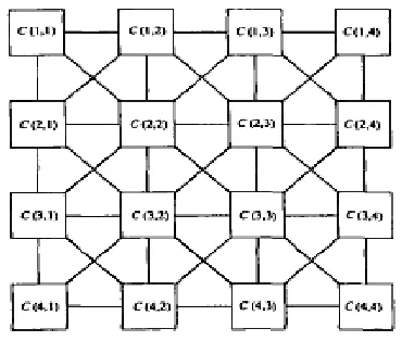
Recently, a novel class of information-processing system called cellular neural networks has been proposed [5].Like neural network [6],it is a large-scale nonlinear analog circuit which processes signals in real time. It is made of a massive aggregate of regularly spaced circuit clones, called
cells, which communicate with each other directly
only through its nearest neighbors. Each cell is made of a linear capacitor, a nonlinear voltage-controlled current source, and a few resistive linear circuit elements. Cellular neural networks share the best features of both worlds; its continuous time feature allows real-time signal processing found wanting in the digital domain and its local interconnection feature makes it tailor made for VLSI implementation.
The CNN is inherently local in nature, so it cannot be expected to efficiently perform global operations of a coding scheme, e.g., entropy coding. However, due to the highly parallel nature of the structure, its speed outperforms traditional digital solutions. The price for this high execution speed is the lower precision of the analog device. The JPEG still image-compression standard and MPEG, the moving image standard have been effectively implemented in the CNN. Spatial sub band coding algorithm is also well suited for the CNN architecture, which is superior to the JPEG for lossless compression both in terms of speed and compression efficiency.
Figure 10 Two Dimensional Cellular Neural Networks
7. CONCLUSIONS
81 wavelets, fractals and predictive coding described in this paper. One of the advantages of doing so is that implementation of various techniques can be standardized on dedicated hardware and architectures. Extensive evaluation and assessment for a wide range of different techniques and algorithms can be conveniently carried out on generalized neural network structures. With dedicated hardware implementation, the massive parallel computing nature of neural networks is quite obvious due to the parallel structure and arrangement of the neurons within each layer. In addition, neural networks can also be implemented on general purpose parallel processing architectures or arrays with programmable capability to change their structures and hence their functionality [10]. At present, research in image compression neural networks is limited to the mode pioneered by conventional technology, namely, information compacting (transforms) +
quantization + entropy coding. Neural networks are only developed to target individual problems inside this mode [9, 1, and 23]. Typical examples are the narrow channel type for information compacting and LVQ for quantization, etc. Although significant work has been done towards neural network development for image compression, and strong competition can be forced on conventional techniques, it is premature to say that neural network technology can provide better solutions for practical image coding problems in comparison with the traditional techniques. Further research can also be targeted to design neural networks capable of both information compacting and quantizing. Hence the advantages of both techniques can be fully exploited. Therefore, future research work in image compression neural networks can be considered by designing more hidden layers to allow the neural networks go through more interactive training and sophisticated learning procedures. Accordingly, high performance compression algorithms may be developed and implemented in those neural networks. Dynamic connections of various neurons and non-linear transfer functions can also be considered and explored to improve their learning performances for those image patterns with drastically changed statistics.
REFERENCES
[1] Christophe Amerijckx et.al, “Image Compression by Self-organized Kohonen maps”, IEEE Trans. on Neural Networks , Vol.9, No.3, May 1998
[2] Michael, F Barnsley, “Fractal image compression”, Notices of the AMS, Vol. 43, No. 6, June 1996, pp 657-662
[3] Jose M Barbalho et.al, “Hierarchical SOM applied to Image Compression”, Proc. IEEE, 2001, pp 442-447
[4] G. Candotti, S. Carrato et al., “Pyramidal multiresolution source coding for progressive sequences”, IEEE Trans. Consumer Electronics,Vol. 40, No.4, Nov.1994, pp 789-795
[5] L. O. Chua and L. Yang, “Cellular neural networks: Theory and applications,” IEEE Trans. Circuits Systems., vol. 35, pp. 1257– 1290, Oct. 1988
[6] L. O. Chua and T. Roska, “The CNN paradigm,” IEEE Trans. Circuits Syst. I, Vol. 40, pp. 47–156, Mar. 1993
[7] J. Dangman, “Complete discrete 2-D Gabor transforms by neural networks for image analysis and compression”, IEEE Trans. on. ASSP, Vol. 36, 1988, pp 1169-1179
[8] T.K. Denk, V. Parhi, Cherkasky, “Combining neural networks and the wavelet transform for image compression”, IEEE Proc. ASSP, Vol. 1, 1993, pp. 637-640
[9] R.D. Dony, S. Haykin, “Neural network approaches to image compression”, Proc. IEEE, Vol. 83, No. 2, Feb. 1995, pp 288-303 [10] W.C. Fang, et. al, “A VLSI neural processor
for image data compression using self-organization networks”, IEEE Trans. Neural Networks, Vol. 3 , No. 3, 1992, pp 506-519 [11] Yuval Fisher, “Fractal iamge Compression-
Theory and application”, Springer-Verlag, New York, 1995
[12] R Gonzalez and R Woods, “Digital Image Processing”, Addison-Wesley, 3rd ed., New
York, 1993
[13] R. Hecht-Nielsen, “Neuro computing”, Addison-Wesley, Reading, MA, 1990
[14] N. Heinrich, J.K. Wu, “Neural network adaptive image coding”, IEEE Trans. On Neural Networks, Vol. 4, No. 4, 1993, pp 605-627
[15] J. Jiang, “Image Compression with neural networks – A survey”, Signal Processing:
Image communication, Elsevier Science B.V., Vol.14, 1999, pp 737-760
82 [17] S J Lee et. al, “Fractal Image compression
using Neural Networks”, Proc.. IEEE, 1998, pp 613-618
[18] R.P. Lippmann, “An introduction to computing with neural nets”, IEEE ASSP Magazine, April 1987, pp 4-21
[19] S.B. Lo, H. Li et al., “On optimization of Orthonormal wavelet decomposition: implication of data accuracy, feature preservation and compression effects”, SPIE Proc., Vol. 27, 07, 1996, pp. 201-214
[20] S.G. Mallat, “A theory for multiresolution signal decomposition: The wavelet representation”, IEEE Transactions on Pattern Analysis & Machine Intelligence, Vol. 11, No.7) July 1989, pp 674-693
[21] C.N. Manikopoulos, “Neural network approach to DPCM system design for image coding”, IEE Proc., Vol. 5 October 1992, pp 501-507
[22] A W H Lee, and L M Cheng, “Using Artificial Neural Network for the calculation of IFS Codes, Proc. of IEEE, 1994, pp 4038-4043
[23] M. Mougeot, R. Azencott, B. Angeniol, “Image compression with back propagation: improvement of the visual restoration using different cost functions”, Neural Networks, Vol. 4, No. 4, 1991, pp 467-476
[24] A. Namphol, S. Chin, M. Arozullah, “Image compression with a hierarchical neural network”, IEEE Trans. Aerospace Electronic Systems, Vol 32, No.1, January 1996, pp 326-337
[25] Mark Nelson, Jean Loup Gailly, “The data compression Book”, 2 ed., M&T Pub.Inc., USA, 1996
[26] N.M.Rahim, T.Yahagi, “Image Compression by new sub-image bloc classification techniques using Neural Networks”, IEICE Trans. On Fundammentals, Vol. E83-A, No. 10, pp 2040-2043, 2000
[27] S.A. Rizvi, N.M. Nasrabadi, “Residual vector quantization using a multilayer competitive neural network”,, IEEE Jl. Selected Areas in Comm. Vol. 12, No.9, December 1994, pp. 1452-1459
[28] Valluru B Rao and Hayagriva V Rao, “Neural Network and Fuzzy Logic”, 2ed. M&T Pub.Inc., USA, 1996
[29] T. Roska and L. O. Chua, “The CNN universal machine: Analogic array computer,” IEEE Trans. Circuits Syst. I, vol. 40, Mar. 1993, pp. 163–173
[30] Peter L Venetianer, Tomas Roska, “Image compression by Cellular Neural Networks”, IEEE Trans. On Circuits and systems –I, Vol.45, No.3, March 1998
[31] Scott Umbaugh, “Computer Vision and Image Processing”, Prentice Hal Intl., Inc., 1988 [32] Eiji Watanbe and Katsumi Mori, “Lossy
Image compression using a modular structured neural network”, Proc. of IEEE Neural Network and Signal Processing Society, XI, Sept 2001
[33] R.B. Yates et al., “An array processor for general-purpose digital image compression”, IEEE Jl. Solid-state Circuits, Vol 30, No.3, 1995, pp .244-250
[34] P. V. Rao, Suhas Madhusudana, Nachiketh S S, and Kusuma Keerthi, “Image Compression using Artificial Neural Networks”, Second International Conference on Machine Learning and Computing, ICMLC2010, Feb 2010, Bangalore, India [35] Pratim Dutta et.al, “Digital Image