Abstract—Simtrade is a computational model that simulates international trade between multiple countries. It predicts the economic status of countries based on purchasing preferences and yearly events. It generates trade activity and tracks the migration of currencies, using that data to predict exchange rates. It also follows the movements of assets and calculates bond ratings. The results are a yearly tabulation of economic aggregates including realistic levels of trade, debt and investment.
Index Terms—Currency migration, trade balance, current account (CA), financial account (FA), exchange rates.
I. INTRODUCTION
Simtrade predicts the economic future of countries based on country definitions and transactions. It tracks production and spending and shows how a portion is allocated to purchase foreign goods. Starting with the basic Y=C+I+G+TB, it shows a year-by-year dispersal of funds into economic aggregates [1] and applies NFIAs and NUTs to calculate the CA.
A matrix model handles the transfers of international assets to derive the FA. Money supplies, reserves and exchange rates are derived for each year. The product of the simulation is the yearly tabulation for each country, each a profile of its economic health and its peoples’ welfare.
To run the program, the user selects which countries to include and how they trade with each other. Each country has attributes that will affect how it fares as a trading partner, and the user can modify the values to vary the outcome.
The transaction file defines the starting date and the trade fractions. The trade is guided by fractions, a set of percents totally to 100 that define how much of the imported goods come from each of the other countries.
Currencies and their values are important; they determine how many goods can be bought with each trading dollar. Many factors contribute to real exchange rates [2], but here they are determined by the dispersion of a country’s money and its assets. The value of the currency is highest when all its currencies and assets are held by its own citizens; lowest when most is held by foreign citizens.
The model tracks both goods as well as trade dollars because money alone could lose or gain value. Goods are a better measurement of welfare for people. It is not significant to state that each person now earns $50,000 compared to$40,000 earned last year without knowing what that money will buy. However, to say that each person now earns 15 units
Manuscript received April 12, 2013; revised June 23, 2013.
T. G. Kennedy is with the North Carolina State University, Raleigh, NC (e-mail: t7k3s7k9@ aol.com).
of goods compared to 12 units last year is a statement of achievement. So each year a matrix of units of goods is calculated to show who receives what quantities of goods.
As the simulator steps through the years, contention for world funds may become problematic. Trade deficits require that money be borrowed, as do government deficits. The simulator seeks funding from any country, but deficit funding is ultimately limited by the world's pool of private savings [3]. A run is successful when there are enough savers in the world to satisfy all the borrowers.
II. DEFINING TRADE PREFERENCES
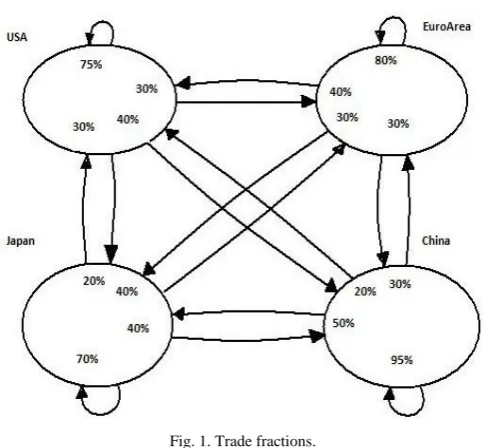
Fig. 1. Trade fractions.
Trade preferences define the pattern of money flows. Trade values will change from year to year but trade patterns will vary much slower, so fractions are used to indicate the portion of trade from each other country. One fraction is MPC Home [4], or marginal propensity to consume home goods; it is the portion of goods that a country buys from its own production. The portion of goods that a country imports is 1-MPCHome.
Each country’s import preferences can be stated as fractions indicating how its imports are split between the rest of the world. In Fig. 1 the USA consumes 75% of its goods from its own country; so MPC Home is .75.Of the 25% that it imports, 30% comes from Euro Area, 40% comes from China, and 30% comes from Japan.
For this model, this information is sufficient to define a country’s trade preferences. Exports definitions are redundant because imports preferences from other countries define the exports. Additionally, because fractions are used Tom Kennedy
instead of defined trade values, trade volumes become a function of production volumes. Increasing production means a country consumes more and imports more, but all are still proportioned by the fractions. This is an important assumption.
III. TWO USER PROVIDED FILES
The World Creation file contains the list of countries and attributes of each. These include population, productivity rate, initial assets and money supply, savings rate, tax rates, government spending rates, marginal propensity to consume, marginal propensity to consume home goods, L-constants and price levels [4].
In the Transaction file, the user states the import fractions and optionally any NFIA, NUT, or KA values. Each entry is a pair of countries and a value. These are persistent settings for the duration of the simulation but can be overridden starting with any year.
IV. RUNNING THE SIMULATOR
The user starts the trading simulator by stating which world he wants simulated and which set of transactions to apply. Also, the user can selectoptions indicating if certain variables are allowed to float such as exchange rates of currencies, units traded, price level, interest rates, MPC Home, and allowing reserves to be transferred to the money supply.
Once the trading world is defined, the simulator steps through the transactions handling all the events for each upcoming year. Trades are attempted by exchanging goods for funds. If funds are not available for purchases, assets or private bonds must be sold. Each country’s accounting is performed for GDP, GNI, GNDI, GNE, TB, CA, S, I, C, FA, units consumed per person, price level, and government revenue and spending. The year is completed by selling government bonds (if necessary), calculating exchange rates and external wealth, and setting bond ratings. (Refer to Fig. 12 and Fig. 13 for example output.)
Certain events can stop the simulation. One is a country attempting to sell private bonds or government bonds and there are not enough funds available from any other country to buy them. Another is one country wanting to import goods from another country that does not have enough goods to sell. The simulator provides no self corrections for these situations: the user-defined countries must either save more, make more, or consume less. However, the user can turn on the options “adjxrate” and “adjunits”, and floating exchange rates will affect the number of units that a country imports, thereby extending the simulation run.
V. TRACKING CURRENCIES
Matrices are used to track the migration of currencies. In Fig. 2 the residence of each country’s currency is shown on each row. For example the US has $3500 in money supply, $3424 in the USA and $76 in China. The currencies residing in each country is shown in each column. In the USA resides $3424 in US dollars, $61 in Euros, and $49 in Japanese yen.
When the simulation starts, all non-zero values are on the diagonal meaning that each country has only its own currency. With each year of trading, the funds are shifted horizontally, indicating currency migration.
Money Supp Resides in______________________________ _n From___ USA Euro AR China Japan
0 USA34240 760 1EuroAr 613109300 2 China00 60000 3 Japan49 01281623
Fig. 2. Residence matrix for currencies.
With real international trade, there are many methods of currency payments [5]. However, this simulator uses this payment order: when country A purchases goods from country B, A uses B’s currency first, then depletes other held foreign currencies, then use sits own currency last. For example, China must give the USA three payments: first $50, then $100, then another $100.Starting from Fig. 2, notice how funds will be moved from the column for China to the column for the USA.
The $50 is taken from the $76 leaving $26.The first $100 takes that $26, the Euro Area’s $30, and $44 of Japan’s $128 (leaving $84). The second $100 takes that $84 and $16 of Chinese yuan leaving $5984.Below Fig. 3 reflects this.
Money Supp Resides in______________________________
_n from ___ USA Euro AR China Japan 0USA35000 00
1EuroAr 91310900 2China16059840 3 Japan177001623
Fig. 3. Final residence matrix for currencies.
Making payments by this ordering means that currencies are returned to their own countries. Most exporters prefer this method [2], and some governments insist on it [6].
In this simulator, exchange rates are determined from the dispersion of a currency into other countries. The first row of Fig. 3 shows that no USA dollars reside in other countries, thus indicating a strong dollar. On the other hand Japan has over 10% of its currency outside Japan, slightly weakening it.
VI. TRACKING ASSETS AND THE FINANCIAL ACCOUNT
The movement of assets into and out of a country determines its financial account. Here, the USA, the Euro Area, China, and Japan have initial assets of $5000, $120000, $100000, and $10000 respectively. Thus, the initial assets matrix only has only those values along the diagonal.
Assets: Owned by______________________________ _n Origin _ USA Euro AR China Japan
0USA2000 02000 1000 1EuroAr0120000 00 2China0 091000 9000 3Japan 00010000
Fig. 4. Asset matrix after USA exported $3000.
The next year, Japan exported $12000 worth of assets to the USA. Fig. 5 above shows how the simulator tracked the assets. Japan’s EXfa is $10000 ($1000 and $9000), and EXha is $2000. USA’s IMha is $1000 and IMfa is $11000.
Assets: Owned by______________________________ _n Origin_ USA Euro AR China Japan
0USA3000020000 1EuroAr01200000 0 2China90000910000 3Japan 2000008000
Fig. 5. Asset matrix after japan exported $12000.
For any country, the financial account is determined by: FAEXhaIMhaEXfaIMfa (1) Since CA plus FA plus KA must sum to zero, this method of asset manipulation to get FA verifies the CA calculations [7].This becomes more apparent in the Example Output.
VII. LOG OF TRADING EVENTS
A log of events is put into a file to help visualize the generated trading activity. Double-entry accounting is used for goods and bonds. Fig. 6 shows a simple $100 trade.
_____________________________________________________
2007 Move Mon Supp from China to USA for $ 100.00 2007 Move Goods from USA to China for $ 100.00
_____________________________________________________
Fig. 6. Entry log of simple trade of money supply for goods.
In this entry, $100moves from China to the USA, and goods move from USA to China.(The $100 could be made up of US dollars, Chinese yuan, or even other currencies.)
_____________________________________________________
2002 Move Corp Bonds from India to Saudi a for $ 20.24 2002 Move Mon Supp from Saudi a to India for $ 20.24 2002 Move Mon Supp from India to Japan for $ 20.24 2002 Move Goods from Japan to India for $ 20.24
_____________________________________________________
Fig. 7. Entry log of selling bonds first and then buying goods.
In Fig. 7 India is buying goods from Japan, but does not have enough money. First it sells corporate bonds to Saudi Arabia and gives that money to Japan. Then, it receives its goods. So the four lines show movements of bonds, money, money again and finally goods, all the result of one trade.
The log entries are actually for net trade amounts. Referring back to Fig. 1, the number of currency flows each year is given by n(n-1) where n is the number of countries. The net trades, however, are half that number, so for Fig. 1 six log entries are created each year of trade.
_____________________________________________________
2018 Move Tbills from Euro Ar to Japan for $145.91 2018 Move Mon Supp from Japan to Euro Ar for $145.91 _____________________________________________________
Fig. 8. Entry log of selling t-bills to fund government debt.
The selling of government bonds is also recorded in the log.
In Fig. 8 the Euro Area has a government debt of $145.91, and Japan has enough money to buy them. So Euro-Bills move to Japan, and money moves to the Euro Area. Each year n log entries can be added for selling bonds.
In the previouslog entries involving bonds, the borrower was able to secure funds from a lender. If a global shortage of funds exists so no single country is able to buy the bonds, an error message appears in the log stating the transaction failed and the simulation stops. The example output in Fig. 12 shows this situation.
VIII. SCENARIOS
Following are two scenarios showing how world trade situations develop. The first applies to currency values and the second to Greece’s currency dilemma.(In both scenarios the initial assets and initial money supplies have been reduced to expedite the financial consequences.)
IX. SCENARIO 1:THE PERIL OF DUAL DEBTS
Four regions define this world: USA, Euro Area, China, and Japan. The USA has a large government deficit and a large trade deficit each year, and both are about the same size. Its government deficit is not covered by its own people, but China covers it. Its trade deficit is also with China. So each year trade dollars end up in China, and China buys the same amount of T-bills [8], [9]. Thus, no US dollars accumulate outside of the USA. And since the simulator uses excess currencies outside a country to determine its exchange rates, exchange rates between the USA and China should not change during this period. The simulator results follow.
Fig. 9. Assets, money supplies and exchange rates for USA and China.
Fig. 9 shows assets on the lower two lines; USA’s assets (in T-Bills)descend from $2000 to zero within seven years, and China’s increases from $2000 to $4200.USA’s money supply (third line from bottom) starts at $5000 and then decreases to $4000starting in year 2007; China’s starts at $10000 and increases slightly.
The top two lines show average exchange rates for both countries starting at 1.0 (using scale on right side).USA’s exchange rate essentially remains constant until 2007 when it drops and ends up at .78.China’s exchange rate decreases
0 0.1 0.2 0.3 0.4 0.5 0.6 0.7 0.8 0.9 1 1.1 1.2
0 5000 10000 15000 20000
2000 2010 2020
exc
hange
ra
tes
assets
mon
ey
su
pp
lies
slightly and then increases to 1.09.
The key here is that USA’s assets were depleted in 2007.So China stopped buying T-bills, and USA’s trade payments started to accumulate in China. This is apparent in the exchange rates; they stayed together for seven years, probably only varying due to trade with the Euro Area or Japan. Then in 2007, USA’s started a 20% decline, which is expected for a country with a trade deficit.
The suggestion is that if country A has a trade deficit with country B for X dollars, and A has an uncovered government deficit larger than X, then B can purchase X dollars of A’s T-bills and keep its own currency from appreciating.
X. SCENARIO 2:GREECE WITH FICTIONAL ATHENA
Eight regions define this world: USA, Euro Area, China, Japan, Luxembourg, Slovakia, Greece and a fictional country Athena. Luxembourg, Slovakia, and Greece have currencies fixed to the Euro. Greece and Athena have identical attributes (assets, population, productivity rate, etc.) and trade preferences, and both have significant government deficits. The exception is that Athena has a floating currency.
Fig. 10. Trade balance and average exchange rate for Greece and Athena.
Fig. 11. External wealth and money supply for Greece and Athena.
Fig. 10 shows the trade balance on the lower two lines; Greece’s descends to -15 and stays at that level. thena’s also descends to -15 but slowly rises back to -7.
The average exchange rate is shown on the upper two lines (using scale on right).Greece’s is fixed to the Euro Area which happens to rise to 1.16 and falls back to where it started. Athena’s just rises to 1.06 and falls significantly. Athena demonstrates normal results for a country with a trade deficit: the exchange rate goes down and the trade balance recovers.
Fig. 11 shows the external wealth on the lower two lines; both jump to 214 but Greece’s descends to -54 and Athena’s descends to 6. The upper two lines show money supply where both start at 150 (using scale on right side). Greece’s descends to 46, but Athena’s only falls to 106. (This run terminated in 2012 with Greece unable to sell private bonds.) The purpose of this scenario is to demonstrate the effect of a common currency for a country like Greece which has a negative trade balance. It is tied to a more prosperous Euro Area, soits exchange rate remains high. Thus, Greece will continue to be burdened with expensive exports that are difficult to sell. Athena has the same trade deficit, but its exchange rate falls, so its exports become attractive. The result after twelve years is that Athena has alargerexternal wealth and has a money supply twice as large as Greece’s.
XI. EXAMPLE OUTPUTS
Fig. 12 (two pages forward) shows the international accounting for the years 2000-2005.GDP drives production for each year and increases with previous investments. The current account, CA, shows a country’s net income. Government’s savings, Sg, is the product of GDP times tax rate minus spending rate. The financial account, FA, shows the assets transferred to cover the CA. Notice how the FA is calculated from the four columns to its left displaying imports and exports of assets. Also, the Balance of Payments Identity, CA+FA+KA=0, holds true. For any year, the world’s CAs sum to zero. The NFIA, NUT, and KA values are taken from the transaction file and applied appropriately. For the USA, notice the large negative TB (trade balance) and Sg (government deficit).For China, notice the large investment, I, due to its high savings rate, and how it causes the GNDI to grow.
Fig. 13 (the last page) shows the economic indicators for the same run. These include estimated bond ratings, floating exchange rates, interest rates and consumption per person. The minimum money supply is a fraction of GNDI that must be met to ensure financial fluidity, a threshold that limits spending. The external wealth, W, is the sum of money supply, assets and T-Bills; the US’s is shrinking, and China’s is growing. Here, USA’s finances aborted the run in 2005.No country would buy its T-bills; it needed $539 (from Fig. 12) but only had $485 in assets to sell at the end of 2004.
Possibilities for a longer life should focus on government deficits, trade patterns, savings rate and productivity.
XII. DISTINCTIONS FROM OTHER MODELS
Simtrade is a temporal model that tracks the flows of goods and funds. It assumes that trade is free, not obstructed by tariffs or shipping distances, andonly bounded by production, consumption, savings and deficits. With just these attributes,
0 0.2 0.4 0.6 0.8 1 1.2
-40 -30 -20 -10 0 10 20 30 40
2000 2005 2010
Exchange
Ra
te
Trade
Bala
nc
e
years
-20 30 80 130
-100 -50 0 50 100 150 200 250
2000 2005 2010
Mon
ey
Sup
ply
Externa
l Wea
lth
it tabulates yearly finances until the first country hits a crisis. At that time, it provides the evidence leading up to that situation.
Most other models evaluate trade policies where proposed quotas and tariffs are analyzed quantitatively for their impact
on employment and welfare. Those models use dynamic simulation of multi-product countries which show the necessary transitions needed to optimize wealth if the proposals are enacted. These models have been refined for years and provide value blere commendations [1].
Fig. 12. International accounting file created for four countries: USA, Euro Area, China and Japan.
Fig. 13. Economic Indicators file created for four countries: USA, Euro Area, China and Japan.
has limited function. For example, it only counts units of one product to measure welfare. Its user interface, a Java command line, is quite basic. Its structure accommodates advanced features like reserves and sticky prices, but it lacks the data for the impact of reserves on exchange rates [9]and the values of damping coefficients on price changes.
It does have useful qualities that are unique. Foremost is its handling of multiple countries along with the preferences between them. Simulations with 16 countries have been run, and it is capable of higher numbers. It handles countries with shared currencies (like the Euro) and allows for the creation of new countries.
Next is transparency. HTML files are generated for viewing internal operations. Frequently, economic models appear as black-boxes providing scant reasons for their results [1], but Simtrade provides logs and intermediate matrices to help the user scrutinize the outcomes. A transaction entry between each pair of trading countries is logged for each year. These include the double-entry accounting for goods and T-Bills shown previously. Also, the interaction between n countries requires holding values in n by n matrices. The set of matrices include trade units, trade dollars, reserve ownership, money residency, assets, T-Bills and exchange rates. The matrices are also logged yearly so users can better understand any developing situations.
Lastly, the tabulated output, even though fabricated, reveals proper international accounting. The calculations of the Current Account from the GNDI and the Financial Account from the asset transfers are correct examples of the national economic aggregates used today [4].As a teaching tool, the Balance of Trade Identity and the Current Account Identity become more understandable when presented along with their supporting values. These output sexemplify the transactions of international trade.
While most economic models provide optimal solutions, this model focuses on avoiding disasters. It provides the results of sustained trade deficits and government policies that benefit the present and jeopardize the future. The goal is to steer all countries to a sustained life while improving the welfare of its peoples.
XIII. CONCLUSION
This model simulates international trade with an emphasis on currency migration. Users can experiment with global preferences and observe situations that lead to one country’s prosperity or another’s demise. A classroom setting is a possible use of its detailed tabulations that could reinforce trading concepts. Another is to formulate a set of scenarios to help predict crises before difficult situations actually arise.
REFERENCES
[1] R. Piermartini and R. Teh, “Demystifying modeling methods for trade policy,” WTO Discussion Papers, Geneva, Switzerland, no. 10, pp. 9-36, Sept. 2005.
[2] M. Friedman and R. Friedman, Free to Choose, 1st ed. New York, N.Y.: Harcourt, Brace, Jovanovich, 1980, ch.1-3, pp. 9.
[3] J. Madura, International Financial Management, 10th ed., Mason, Ohio:
South-Western, 2010, ch.18-20.
[4] R. Feenstra and A. Taylor, International Economics, New York, N.Y.: Worth Publishers, 2008, ch.12-20.
[5] J. O. Wijnholds and L. Sondergaard, “Reserve accumulation Objective or by-product,” ECB Occasional Paper Series, Geneva, Switzerland, no. 73, pp. 8-34, Sept. 2007.
[6] M. Jacques, When China Rules the World, 2nd ed., New York, N.Y.:
Penguin Group, 2012, ch.6-13.
[7] R. Feenstra and A. Taylor, International Macroeconomics, 2nd ed.,
New York, N.Y.: Worth Publishers, 2012, ch.3- 4, pp. 10.
[8] Y. Wen, “Explaining China’s trade imbalance puzzle,” Federal Reserve Bank of St. Louis Working Paper Series, St. Louis, MO, no. 2011-018A, pp. 1-14, August 2011.
[9] J. Caruana, “Why central balance sheets matter,” Keynote Address, Bank of Thailand BIS Conference, bis.org, Dec. 2011.