Understanding SIFT Algorithm and its uses
Ms. Samantha Cardoso Mr. Vaibhav Naik
Assistant Professor UG Student
Department of Electronics and Telecommunication Department of Electronics and Telecommunication
Don Bosco College of Engineering,Fatorda, Goa, India Don Bosco College of Engineering,Fatorda, Goa, India
Mr. Sahil Khorjuvenkar Mr. Sairaaj Shirodkar
UG Student UG Student
Department of Electronics and Telecommunication Department of Electronics and Telecommunication
Don Bosco College of Engineering,Fatorda, Goa, India Don Bosco College of Engineering,Fatorda, Goa, India
Mr. Akshat Pai UG Student
Department of Electronics and Telecommunication
Don Bosco College of Engineering,Fatorda, Goa, India
Abstract
The Scale Invariant Feature Transform [1] (SIFT) is an algorithm in image processing to detect and describe local features in an image. It takes an image and transforms it into a collection of local feature vectors. Each of these vectors is supposed to be different and distinctive and also invariant to scaling, rotation or translation of the image. In real-time applications these features can be can be used to find distinctive objects in different images and the transform can be extended to match certain areas in images. This document describes the basic implementation of the SIFT algorithm in various applications and also highlights a potential direction for future research.
Keywords: Difference of Gaussian, extrema detection, key point localization, SIFT algorithm
________________________________________________________________________________________________________
I. INTRODUCTION
Scale-Invariant feature transform (SIFT) is an image descriptor for image based matching and recognition. The SIFT descriptor is invariant to translations, rotations and scaling transformations in the image domain and robust to moderate perspective changes and illumination variations. In its original formulation, the SIFT descriptor comprised a method for detecting interest points from a grey-level image at which statistics of local gradient directions of intensities were accumulated to give a summarizing description of the local image structures in a local neighborhood around each interest point, with the intention that this descriptor should be used for matching corresponding interest points between different images. Later, the SIFT descriptor has also been applied at dense grids which has shown a better performance for tasks like object categorization, texture classification, image alignment and biometrics.
Object recognition (face recognition, coin recognition, identification of vegetation, etc.) is becoming increasingly important for several applications like human-machine interfaces, multimedia, security, communication, visually mediated interaction and anthropomorphic environments. One of the most challenging problems is that the process of identifying an object from a particular scene has to be performed differently for each image, as there are so many conflicting factors altering the object appearance. Our aim is to derive SIFT features from an image and try to use these features to perform object identification.
II. SIFT ALGORITHM
Scale Space Extrema Detection:
This is the first step of the SIFT algorithm. It commences with the detection of points of interest known as key-points in the SIFT framework. At various scales the image is convolved with Gaussian filters and then the difference of successive Gaussian-blurred images are taken. From the Difference of Gaussians (DoG) occurring at multiple scales, the keypoints are chosen as maxima/minima. Specifically, a DoG image D(x, y, σ) is given by
D(x, y, σ) = L(x, y, kiσ) − L(x, y, kjσ) (1)
Where L(x, y, kσ) is the convolution of the original image I(x, y) with the Gaussian blur G(x, y, kσ) at scale and is given as L(x, y, kσ) = G(x, y, kσ) ∗ I(x, y) (2)
Thus a DoG image between scales kiσ and kjσ is basically the difference of the Gaussian-blurred images at scales kiσ and kjσ.
categorized by octave (an octave corresponds to doubling the value of σ), and the value of ki is chosen such that we obtain a fixed
number of convolved images per octave. Then the DoG images are taken from adjacent Gaussian-blurred images per octave. After the DoG images are obtained, the key-points are seen as local minima/maxima of the DoG images across scales. This is achieved by comparing each pixel in the DoG images to its 8 neighbors at similar scale and 9 corresponding neighboring pixels in each of the neighboring scales. A particular key-point called the candidate key- point is selected if the pixel value is the minimum or maximum among all compared pixels.
Keypoint localization:
In the previous step, the scale space extrema detection generates many key-point candidates among which some are unstable. The next step in this algorithm is to perform a detailed fit to the nearby data for precise location, scale and ratio of principal curvatures. As per this information, points that have low contrast (sensitive to noise) or are poorly localized along an edge are rejected.
Interpolation of Nearby Data for Accurate Position:
For every candidate key-point, interpolation of nearby data is used to accurately find its position. Initially, the approach was to locate each key-point at the location and scale of the candidate key-point [1]. The new approach was to calculate the interpolated
location of the extremum which improved matching and stability substantially [2]. Interpolation is achieved with the help of the
quadratic Taylor expansion of the Difference-of-Gaussian scale- space function, D(x, y, σ) with origin as the candidate keypoint. This Taylor expansion is given by:
D(X) = D +∂D
T
∂X X +
1
2X
T∂ 2D
∂X2X (3)
Where D and its gradients are calculated at the candidate key-point and X= (x, y, σ) is the offset from this key-point. The location of the extremum x̂, is found by taking the derivative of this function with respect to X and setting it to zero. If offset x̂ is larger than 0.5 in any respective dimension, then it shows that the extremum is lies closer to another candidate keypoint. The candidate key-point is thus changed and the interpolation is performed instead about that point. Another option is to add the offset to its candidate key-point to get the interpolated estimate for locating the extremum.
Discarding Low Contrast Key-Points:
Key-points with low contrast value are to be discarded when the value of the second-order Taylor expansion D(X) is computed at x̂. If this value is smaller than 0.03, the candidate key-point is discarded. Otherwise it is considered by taking the final scale- space location y+ x̂, where y becomes the actual location of the keypoint.
Eliminating Edge Responses
Along the edges, the DoG function will have appreciable responses, even if the candidate key-point is not robust to small amounts of noise. Thus to improve stability we eliminate key-points having poorly determined locations but considerably high edge responses.
In the DoG function, for peaks having poor definitions, the principle curvature across the edge is much larger than the principle curvature along it. We find these principle curvatures by solving for the eigen values of the second-order Hessian matrix, H:
H = [Dxx Dxy
Dxy Dyy] (4)
The Eigen values of H are proportional to the principle curvatures of D. It is sufficient for SIFT’s purposes if γ = α β⁄ , considering α to be greater than β. The sum of the 2 Eigen values is given by the trace of H (Dxx + Dyy) whereas the product is determined from its determinant (DxxDyy− Dxy2 ). the ratio R can be proved to be equal to(γ + 1)2⁄γ, which depends on the ratio
of Eigen values rather than their individual values. R is least if the Eigen values are equal to each other.
Here R is (Trace of H)2⁄Determinant of H. thus, higher the absolute difference between the 2 Eigen values, which is similar
to a high absolute difference between the principle curvatures of D, higher the value of R. which implies a possibility of a candidate keypoint being poorly localized and therefore rejected if R for that key-point is larger than (γth+ 1)2⁄γth, for some
threshold Eigen value ratio γth. The new approach makes use of γth = 10.[2]
Orientation Assignment:
In this step respectively, each and every key-point is assigned one or more orientations depending on local image gradient directions. To achieve invariance to rotation, this is the most important step as the key-point descriptor can be shown relative to this orientation and thus achieves invariance to image rotation.
For all computations to be performed in a scale-invariant manner, the Gaussian- smoothed image L(x, y, σ) at the key-point’s scale σ is considered. For an image sample L(x, y) at scale σ, the magnitude of gradient, m(x, y), and orientation, ϴ(x, y), are found using differences of pixels as follows:
m(x, y) = √(L(x + 1, y) − L(x − 1, y))2+ (L(x, y + 1) − L(x, y − 1))2 (5)
ϴ(x, y) = tan−1((L(x, y + 1) − L(x, y − 1)/(L(x + 1, y) − L(x − 1, y)) (6)
Fig. 1: A particular key-point Fig. 2: Gradient magnitudes and orientation from Gaussian-blurred image
The size of the orientation collection region around a certain key-point depends on its scale. In short, larger the scale, larger the collection region.
An orientation histogram consisting of 36 bins is formed with each covering 10˚. A particular sample in the neighboring window is measured by its gradient magnitude along with a Gaussian-weighted circular window with σ that is 1.5 times that of the key-point scale. Dominant orientations correspond to peaks in this histogram. When the respective histogram is filled, the orientations regarding the highest peak and the local ones that are within 80% of the highest peaks are assigned to the key-point. When multiple key-points are assigned, an extra key-point is generated having the same location and scale as that of the original for each additional orientation.
Fig. 3: Example of a generated Histogram consisting of 36 bins
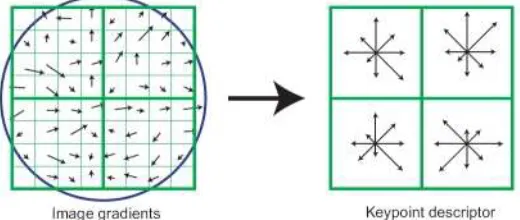
Key-Point Descriptor:
Previously in this algorithm, key-point locations at specific scales were found followed by assigning orientations to them. This ensured invariance to image location, scale and rotation. In this step of the algorithm, a descriptor vector for each key-point is computed such that the descriptor is highly distinctive and partially invariant to the remaining variations such as illumination, 3-D viewpoint, etc. This step is executed on the image nearest in scale to the key-point’s scale.
Firstly, on 4 X 4 pixel neighborhoods containing 8 bins each, a set of orientation histograms is generated. The histograms are calculated using magnitude and orientation values of samples in a 16 X 16 region around the key-point such that each histogram consists of samples from a 4 X 4 sub-region of the original neighborhood region. The magnitudes are further weighted by a Gaussian function with σ equal to one half the width of the descriptor window. From all the values of these histograms, a descriptor forms into a vector which is normalized to unit length in order to enhance invariance to illumination.
III. APPLICATIONS OF SIFT ALGORITHM
Object recognition using SIFT features:
Due to SIFT’s ability to detect distinctive key-points that do not depend on location, scale and rotation, and robust to changes in position and illumination, they are useful in object recognition. The steps are given below:
Using the algorithm given above, SIFT features are obtained from the input image.
These features are matched to the SIFT feature database which is obtained from training images. This feature matching is achieved using Euclidean-distance closest neighbor approach. To improve robustness, matches for the key-points whose ratio of the nearest distance to the second nearest neighbor distance is larger than 0.8 are rejected. This deletes many of the false matches arising from a background clutter. To avoid tedious search of finding the Euclidean-distance-based nearest neighbor, an algorithm known as the best-bin-first algorithm is used.[3]
Although many of the false matches were discarded from background clutter, there still exist matches that belong to different group of objects. Thus to increase robustness for object identification, we would want to collect the features belonging to the same object in a group and reject those matches that were left out during the clustering process. This is done using the Hough transform, which basically identify clusters of clusters of features that belong to the same object. The set of object poses that are consistent with the key-points’ location, scale and orientation get a vote from the key-point itself. Candidate objects are thus identified only when bins accumulate at least 3 votes.
For each candidate cluster, a solution of least square s is obtained for the best estimated affine projection parameters linking the training image to the input image. If a key-point projection lies within half the error range which was used for parameters in the Hough transform bins, the key-point match is kept. If less than 3 point remain, the object match is rejected.
A recent approach was proposed regarding the use of SIFT descriptors for multiple object detection purposes.[4] This is tested
on aerial and satellite images.
Robot Localization and Mapping:
In this application respectively,[5]a trinocular stereo system is used to find 3D estimates for specific keypoint locations. Only
when keypoints appear in all 3 images with consistent disparities are they used, resulting in few outliers.
When the robot is in mobility, it localizes itself by making use of feature matches to the presently existing 3D map, and then consequently adds features to the map. This creates a robust and accurate solution to the problem of robot localization in unknown territories and environments.
Panorama Stitching:
This application makes use of SIFT feature matching techniques in image stitching for a fully automated panorama reconstructed image from non-panoramic images. The SIFT collected from different input images are matched against each other to locate k nearest neighbors for each and every feature. These features are correspondingly used to find m candidate matching images for each image. Homographies (bijection that maps lines, and thus a collineation) between are then found and a probabilistic model is used for verification purposes. Since input images do not have any restriction, a typical graph search is used to find connected components of respective image matches. Here, each connected component will correspond to a panorama. Due to this SIFT inspired object recognition approach to panorama stitching, the end result is insensitive to the ordering, orientation, scale and illumination of the images. Multiple panoramas and noise images (not part of the composite image) may be contained in original input images, thus recognizing panoramic sequences and rendering the final image as output.[6]
3D Scene Modeling, Recognition and Tracking:
for a certain virtual projection and final rendering. To reduce the jitter in the virtual projection, a regularization technique is used.[7] For actual 3D object recognition and retrieval, 3D extensions have also been evaluated.[8][9]
Analyzing the Human Brain in 3D Magnetic Resonance Images:
The Feature-based Morphometry (FBM) technique [10] makes use of extrema in a DoG scale-space to analyze and classify 3D
magnetic resonance images (MRIs) of the human brain. FBM creates or models an image as a combined collage of independent features, conditional on image geometry and group labels. At first, features are extracted in individual images from a 4 dimensional DoG scale-space, after which it is modeled with respect to their appearance, geometry and group co-occurrence statistics across a set of images.
IV. CONCLUSION
The SIFT algorithm is quite useful and formidable in real life applications, giving accurate and efficient results. Further studies are being done to make better use of this algorithm in the future and searching for ways to improve its efficiency in scenarios containing variations in illumination.
REFERENCES
[1] Lowe, David G. (1999). “Object recognition from local scale-invariant features”. Proceedings of the International Conference on Computer Vision. pp. 1150-1157.
[2] Lowe, David G. (2004). “Distinctive Image Features from Scale-Invariant Key-points”. International Journal of Computer Vision 60 (2): 91-110.
[3] Beis, J.; Lowe, David G. (1997). “Shape indexing using approximate nearest-neighbor search in high-dimensional spaces”. Conference on Computer Vision and Pattern Recognition, PuertoRico: sn. pp. 1000-1006.
[4] Beril Sirmacek and Cem Unsalan (2009). “Urban Area and Building Detection Using SIFT Keypoints and Graph Theory”. IEEE Transactions on Geoscience and Remote Sensing 47 (4): 1156-1167.
[5] Se, S.; Lowe, David G.; Little, J. (2001). “Vision-based mobile robot localization and mapping using scale-invariant features”. Proceedings of the IEEE International Conference on Robotics and Automation (ICRA). p. 2051.
[6] Brown, M.; Lowe, David G. (2003). “Recognizing Panoramas”. Proceedings of the ninth IEEE international Conference on Computer Vision. pp. 1218-1225.
[7] Iryna Gordon and David G. Lowe, “What and where: 3D object recognition with accurate pose”, in Toward Category-Level Object Recognition, (Springer-Verlag, 2006), pp. 67-82.
[8] Flitton, G.; Breckon, T. (2010). “Object Recognition using 3D SIFT in Complex CT Volumes”. Proceedings of the British Machine Vision Conference. pp. 11.1-12.
[9] Flitton, G.T., breckon, T.P., Megherbi, N. (2013). “A Comparison of 3D Interest Point Descriptors with Application to Airport Baggage Object Detection in Complex CT Imagery”. Pattern Recognition (Elsevier).