www.atmos-meas-tech.net/9/215/2016/ doi:10.5194/amt-9-215-2016
© Author(s) 2016. CC Attribution 3.0 License.
Non-parametric and least squares Langley plot methods
P. W. Kiedronaand J. J. Michalsky1
1Cooperative Institute for Research in Environmental Sciences, University of Colorado,
and Earth System Research Laboratory, National Oceanic and Atmospheric Administration, Boulder, USA
aformerly at: the Cooperative Institute for Research in Environmental Sciences, University of Colorado,
and Earth System Research Laboratory, National Oceanic and Atmospheric Administration, Boulder, USA Correspondence to: J. J. Michalsky ([email protected])
Received: 25 February 2015 – Published in Atmos. Meas. Tech. Discuss.: 27 April 2015 Revised: 10 December 2015 – Accepted: 15 December 2015 – Published: 25 January 2016
Abstract. Langley plots are used to calibrate sun radiome-ters primarily for the measurement of the aerosol component of the atmosphere that attenuates (scatters and absorbs) in-coming direct solar radiation. In principle, the calibration of a sun radiometer is a straightforward application of the Bouguer–Lambert–Beer lawV =V0e−τ·m, where a plot of
ln(V )voltage vs.mair mass yields a straight line with in-tercept ln(V0). This ln(V0)subsequently can be used to solve
for τ for any measurement ofV and calculation ofm. This calibration works well on some high mountain sites, but the application of the Langley plot calibration technique is more complicated at other, more interesting, locales. This paper is concerned with ferreting out calibrations at difficult sites and examining and comparing a number of conventional and non-conventional methods for obtaining successful Langley plots. The 11 techniques discussed indicate that both least squares and various non-parametric techniques produce sat-isfactory calibrations with no significant differences among them when the time series of ln(V0)’s are smoothed and
in-terpolated with median and mean moving window filters.
1 Introduction
Langley plots are used to determine the instrumental con-stant V0, i.e., to calibrate, sun radiometers from a series of
measurementsVi at various air massesmi. According to the
Bouguer–Lambert–Beer (BLB) law, the optical depthτis de-termined from pairs of points (Vi, mi)that are fit to the linear
equation
ln(V )=ln(V0)−τ·m. (1)
Ifτ is constant, the equation defines a straight line; the graph is called a Langley plot. When data are not perfect and con-tain outliers (τ is not always the same for all measurements when timet and air massm(t )change), the Langley plot is obtained after removing the outliers. Thus, one can still ob-tainV0from Eq. (1). The derived instrumental constantV0, if
valid, is used to retrieve the optical depthτ (m)for any mea-suredV and calculatedm:τ (m)= −m−1ln(V/V0). The main
purpose of sun radiometry is to retrieve the optical depth of atmospheric constituents, mainly aerosols, but also O3, CO2,
SO2, H2O, etc. from the direct beam’s atmospheric
transmit-tanceV /V0.
After multiplying the transmittance by the extraterrestrial solar flux, one obtains the flux measured by the instrument. The flux at the site of the measurements can be used, e.g., to validate radiative transfer models (Mlawer et al., 2000). The multi-filter rotating shadowband radiometer (MFRSR) (Harrison et al., 1994) and the rotating shadowband spectro-radiometer (RSS) (Harrison et al., 1999) measure the diffuse components of the flux, as well as the direct components. These instruments were calibrated via the Langley method and with standard lamps (Kiedron et al., 1999). Schmid and Wehrli (1995) concluded that when retrieving optical depth the calibration with Langley plots (Langleys) is superior to the calibration based on standard light sources; however, the quality of calibration by Langleys depends on the site at which the instrument is located.
The Langley plot method of calibration consists of locat-ing a subset of raw data points (ln(Vi), mi)to which a straight
line can be fit. The intercept of the straight line estimates the calibration constant ln(V0). This is a consequence of the BLB
τi require verification and correction if the sun radiometer
was poorly calibrated or its calibration has drifted. The BLB law implies that the slope of the straight line fitted to points τi,1/mi estimates the calibration constant correction factor
(Cachorro et al., 2004, 2008). Finding this slope is a mathe-matically equivalent approach to finding the intercept in the Langley plot method. In both approaches the calibration suc-cess hinges on correctly locating the subset when the optical depth of atmosphere is constant.
It is often overlooked, that the presence of the straight line in the data set ln(Vi), mi orτi,1/mi does not imply that the
actualτ is constant. The existence of a straight-line fit is the necessary condition but not a sufficient one for the constancy of the optical depth. Shaw (1976) may have been the first to point this out. He observed that in cases when the op-tical depth of aerosols is a parabolic function of time the pairs ln(Vi), mi create a perfect straight line, but its
inter-cept is not the actual ln(V0). Then the intercept is biased, and
thus it cannot be used as a calibration constant. Several au-thors – Tanaka et al. (1986), Nieke et al. (1999), Harrison et al. (2003), and Campanelli et al. (2004) – mention this prob-lem more or less explicitly. More recently, Marenco (2007) devoted his paper to this phenomenon. Equation (1) implies that when the actualτAcontains a varying component that is
inversely proportional to the air mass
τA=τ+ε/m, (2)
the data align along the straight line with a slope τ, but the intercept is now ln(V0)−ε. The hyperbolic dependence 1/m
produces a straight line.
The time series of ln(V0)’s over several days are used to
weed out cases whenεis not zero and estimate the true cali-bration. An individual Langley plot cannot identify the value ofε. The data (ln(Vi), mi)do not contain information on the
presence of a nonzeroε.
The process of removing outliers from the Langley plot may actually facilitate selecting a straight line from the data that will contain a spurious value ofε. Different methods of removing outliers may cause an inadvertent selection of a different value ofε, some larger and some smaller (positive or negative).
We will call a Langley plot with a nonzeroεan anomalous Langley plot. The anomalous Langley plot cannot be identi-fied because data (ln(Vi), mi)do not contain information on
the presence of a nonzeroε. Statistical analysis of the time series of intercepts ln(V0)−εleads to a better estimate of the
calibration constant ln(V0)=<ln(V0)−ε>=ln(V0)−<ε>,
where < > denotes an average used in time-series analysis that usually is a combination of mean and median moving av-eraging windows. When the statistics ofεis unbiased,<ε> tends to zero as the number of samples in the time series in-creases.
Mountaintops like Mauna Loa in Hawaii or Izaña on Tenerife provide environments where the constancy of the
optical depth (ε=0) is frequent. With a small standard de-viation SD(ε)at mountaintops a smaller number of Langleys is necessary to achieve the desired precision of calibration. A long history of measurements at sites like Mauna Loa also warrants the belief that the statistics ofεthere is considered to be unbiased. Thus, within the range of validity of this be-lief an accurate calibration is possible.
In most places where sun photometers are deployed, peri-ods of stable atmospheres are much less common, and they are frequently interrupted by cloud passages, changes in at-mospheric conditions like varying humidity that promulgate aerosol size changes and by aerosol plume incursions. Large numbers of outliers call for special Langley plot analyses going beyond standard straight-line fitting procedures. The statistics ofεis likely to be biased with a large standard de-viation SD(ε). This necessitates a larger number of points in the time series to achieve a desired precision while the fre-quency of Langley events at sites like these is low. There is no guarantee that the statistics ofεis unbiased. It should be emphasized that the difference between easy sites like moun-taintops and difficult sites like Billings, Oklahoma, is quan-titative, not qualitative. The same statistical analysis of time series must be applied in both cases; however, precision and accuracy of results will differ.
When there are no other available independent measure-ments, time-series analysis is the only option for in situ cal-ibration of sun photometers. Photometers that also measure aureole radiance simultaneously with direct solar flux can be calibrated when optical depth is not constant (Tanaka et al., 1986; Nieke et al., 1999; Zieger et al., 2007). These meth-ods can identify anomalous Langley events and estimate the value ofε. Then, in principle, a single Langley is sufficient.
The main objective of the paper is to analyze the efficacy of non-parametric and least squares methods of straight-line fitting to identify Langley plots useful for calibration. We use time-series analysis only to determine the impact of the methods on the estimated calibration constant. While we are not concerned with the identification of anomalous Langley plots, their presence is manifested in outliers of the time se-ries. We do not deal with minor issues related to the differ-ences in air mass among various air constituents: aerosols, ozone, and molecular scattering, in particular, and higher-order effects like atmospheric refraction’s dependence on wavelength impact air mass. In other words, we presume that the BLB as given by Eq. (1) is valid.
plot even if we understand their physical origins. We do not know the statistics of ln(V0)’s in a time series of them, but we
still want to get the best estimate of the calibration constant of a sun photometer.
For simplicity of notation in the rest of the paper Eq. (1) is replaced with a linear equation:
y=α+βx.wherey=ln(V ), x=m, α=ln(V0)andβ= −τ.
The organization of the paper is as follows. In Sect. 2 we define a Langley plot. In Sects. 3 to 7, 11 methods of finding a Langley plot are described: in Sect. 3, two least squares methods; in Sect. 4, the so-called objective algorithm method; in Sect. 5, four non-parametric regressions meth-ods following Theil (1950) and Siegel (1982); in Sect. 6, a non-parametric method of identifying outliers and a modi-fied Siegel (1982) method with sequential removal of out-liers; and in Sect. 7, a method of analyzing histograms of slopes and intercepts. In Sect. 8 we describe the set of data used in the comparisons for all methods. Section 9 presents results of these analyses and comparisons. The final section summarizes the paper.
2 Our definition of a Langley plot
For any set of pointsP = {(xi, yi):i=0, . . ., n−1}and for
any nonnegativeδfind a subsetL⊂P for which a liney= α+βxcan be defined such that one of the following metrics
1=
v u u t
1 k
k−1 X
j=0
rj2or 1 k
k−1 X
j=0 rj
or max
j rj
(3)
that measures the magnitude of residuals is smaller than δ(1<δ)on the setL, where therj=yj−α−βxjare
resid-uals andkis the number of points in the subsetL. We refer to the points of the subsetLasδ-collinear. The subsetLis not unique, or it may not exist whenδ is too small, ignor-ing subsets consistignor-ing of two points only. Therefore, we add a requirement that Lshould be the largest subset with this property of residuals. In other words, a Langley plot is the most numerousδ-collinear subset of setP. The size of the set L(i.e., the number of points that “actually” define the line) is important in judging the viability of the resulting Langley plot (i.e., the subsetL). The quotation marks around “actu-ally” are justified for non-parametric methods, because they do not identify outliers explicitly.
This problem is related to the pattern recognition problem. The human eye and mind are able to solve the problem in a qualitative way very quickly by identifying points that are ap-proximately collinear. The human eye and mind can perform this task regardless of the plot orientation. The result is rota-tionally invariant: neither of the axesx or y is treated pref-erentially. Furthermore, the human eye and mind can almost
instantaneously identify a data setP that has no potential of containing any subsetLof a significant size and rejects this case as not providing a viable Langley plot. Mathematically this problem reduces to the straight-line fit and to a method of identifying and removing outliers. Any one of the crite-ria (Eq. 3) can be used to define the quality of the fit.
Some researchers (Augustine et al., 2003) seemingly avoid the issue of removing outliers altogether by selecting clear-sky days based on the method of Long and Ackerman (2000) for which measurements from collocated broadband shaded and unshaded pyranometers are required. This approach, while effective, misses many Langley plots from partially clear days, so it does not fit the scope of this paper. Further-more, many sites with sun radiometers do not have collocated shaded and unshaded pyranometers.
3 LSF with sequential removal of outliers (SRO)
This is the most straightforward and, probably, the most com-monly used method in existence. The least-square fit (LSF) is applied to the set of points P, and the largest residual (negative or positive) is removed. Then the root mean square (rms) of residuals is calculated. The process is repeated until rms≤rmsmaxand the number of remaining pointsk≥kmin,
with rmsmaxandkmin chosen based on experience. Usually,
most of the outliers are negative (e.g., cloud passages), but there are less frequent cases when the atmosphere has peri-ods of stability at largerτthat may be temporarily interrupted by a cleaner air mass. For this case the outliers at smallerτ are positive. For this reason the method must allow removal of the positive outliers. On our data set we note that we ob-tained good results (meaning that both the number of false and missed identifications of Langley plots were small) when about every fifth outlier that was removed was a positive one. However, we do not claim the value of five is a general rule. Usually measurements with sun radiometers are per-formed at equal time steps. This means that the values of x, the air masses, are not evenly distributed. For 1-minute intervals1x atx=2 might be 10 times smaller than1xat x=6 at midlatitudes, where the air massxis the Rayleigh air mass (Kasten, 1965). Some researchers recognized the bias introduced by the uneven distribution ofx onαdue to the larger number of points at low air masses. For example, For-gan (2000) performed Langley plots on(y/x,1/x)for his sun photometric studies. In the Dobson ozone spectropho-tometer community Langley plots for the ozone extraterres-trial constant (ETC) are performed in coordinates(y/x,1/x) to give a smaller weight to points that are more sparse at large air masses (Dobson and Normand, 1958). Note, how-ever, that for the Brewer UV ozone spectrophotometers the standard equationy=α+βxis used (Redondas, 2005; Ito et al., 2014).
applying weightsw=1/x2to the LSF of the original equa-tion y=α+βx. Herman et al. (1981) considered applying other weighting methods.
A sequential removal of outliers can be applied and the method may have the same terminating criterion in terms of rms < rmsmax; however, the residuals must be calculated for
the equationy=α+βx.
We label these two methods LSFSRO−x and LSFSRO−
1/x, where the subscript SRO stands for “sequential removal of outliers”.
4 The objective algorithm of Harrison and Michalsky
We describe some aspects of the objective algorithm (OA) because (a) its development is an excellent example of how a mathematical method was stimulated by the human eye-and-mind approach, (b) it is based on physical phenomena that are responsible for the curve shape and the outliers, and (c) it is basically a non-parametric method despite the fact that LSF is used for the final filtering.
When Harrison and Michalsky (1994) developed the OA they tested it by comparing a set of cases from 384 days using 500 nm channel data where α andβ were obtained by the eye-and-mind method of Michalsky, who disqualified the non-viable cases and identified the ones that, after the removal of outliers, produced Langley plots. Then he per-formed the LSF on the retained points. The OA did not try to produce “an artificial intelligence” emulating Michalsky’s approach. Instead it identified several physical phenomena (like cloud passages, overcast skies, curvature in the plot, etc.) that were responsible for outliers and the non-linearity of the Langley plots. This justifies the term “objective” in the method’s name. The method applies consecutive filters: each meant to deal with outliers produced by one of the identi-fied physical phenomena that produced them. The last filter is LSF that shaves off outliers larger than 1.5 of the standard deviation of all residuals of points that survived the previous filtering.
The successful Langley plot for the OA is the one for which rms≤0.006 (of retained residuals) and thek/n≥1/3. The value of rmsmax=0.006 was chosen to maximize the
agreement with the eye-and-mind Michalsky method using 143 cases of successful Langley plots. The value of rmsmaxis
valid for the wavelengthλ=500 nm. For other wavelengths the rmsmaxwill be different because aerosols’ impact on
out-liers is wavelength dependent.
5 Non-parametric fits (NPFs)
LSFs use means of{xi}, {yi},{xi,2}, and{yi,xi}. The so-called
breakdown point of the mean is 0 %: a single outlier can sig-nificantly change the value of a mean. On the other hand, the breakdown point of a median is 50 %. Theil (1950) opened
the field of the so-called non-parametric regression fits that are based on medians and, thus, are much more robust.
The setP produces annxnmatrix of all possible slopes
{bi,j}, wherebi,j =(yi−yj)(xi−xj). The matrix is
symmet-ric with a diagonal that has indeterminate values. Its upper or lower triangles each haven(n−1)/2 points. They are used to calculate the slope:
β=med
i<j
bi,j . (4)
From the slopeβthe intercept is obtained also as a median: α=med
i
{yi−βxi}. (5)
Theil’s (1950) algorithm robustness is 29.3 %, which means that when outliers exceed 29.3 % of all points the perfor-mance of the algorithm is not guaranteed; at this level it reaches its breakdown point. The increase of robustness to 50 % was achieved by Siegel (1982) with his method of “re-peated medians” that uses two medians in Eq. (4) rather than one: one median along the rows of the matrix{bi,j}and then
the median of this column of medians β=med
i
med
j {bi,j}
, (6)
where alln(n−1)values of the matrix{bi,j}are used.
The Langley plot is chiefly concerned with obtaining the intercept and, unlike Theil’s focus, the slope is secondary. Instead of obtaining the slope first, one can obtain the inter-cept first. From the matrix {ai,j}of interceptsai,j =(yjxi− yixj)/(xi−xj), one gets the interceptαwith Eqs. (4) or (6)
and then gets the slope from β=med
i
yi−α xi
. (7)
The weighted median methods (Jaeckel, 1972) can also be applied. The uncertainty of slopes bi,j stems from the
measurement errors of yi values. The uncertainty is
in-versely proportional to |xi−xj| if uncertainties for yi are
the same. When |xi−xj| is small, the measurement
er-rors have inversely proportional 1/|xi−xj|larger impact on
the slope. For the intercepts the weights for ai,j are
pro-portional toxi−xj
/(xi2+xj2)1/2. The exact formulas for
using weighted medians for Theil (1950) methods can be found in Birknes and Dodge (1993). The weighted medi-ans, one would expect, should offer an advantage whenxi’s
are not uniformly distributed, which is exactly the case for air masses. However, our simulations with weighted medians did not confirm this expectation. In fact, in our experience the weighted median methods introduced unacceptable biases in αandβ.
β in LSF methods are closed-form formulas derived from smooth analytic functions. The NPF methods are inherently discrete. They depend on medians. The “granulation effect” in a small data sample may lead to errors because of discon-tinuities. The residuals from the LSF methods are unbiased (sum of residuals equals zero), while this is not guaranteed for the methods based on the discreet processes. Theil (1950) and Siegel (1982) NPF methods do not identify outliers ex-plicitly.αandβare generated for any setP, but the outliers must be identified to get the value of the metrics and reach the decision of whether these particularαandβdefine a Langley plot or not. The last problem we solved by using the follow-ing method of outlier identification.
For a given αand β we sort all points according to the ascending value of their residuals (rj≤rj+1). Then we
cal-culate the root mean square of residuals (rmsJ)of the first j =0, . . ., J−1 points. We findJ for which rmsJ ≤rmsmax
and rmsJ+1> rmsmax. All points with indicesj≥Jare
con-sidered outliers. Points with indicesj<Jare retained. They define the Langley plot, which is considered to be successful whenJ≥n/3. Residuals of retained points can be de-biased by performing a LSF on them. This reduces the value of rmsJ
and slightly changesαandβ.
We chose to use rms (the first criterion in Eq. 3) because the data set for OA, which is used in comparisons, is based on rms metrics. The method of identifying outliers in the set P, whenαandβ are given, we label OSM (outlier sorting method). In Sect. 9 we also apply the OSM to the results obtained from the OA method.
We described four NPF methods of finding a Langley plot. We label them as TOSM-β, TOSM-α, SOSM-β, and SOSM-α,
where T and S stand for Theil and Siegel, respectively, andα andβstand for the “intercept-first” and “slope-first” methods and OSM for the outlier sorting method with a final residual de-biasing LSF. The de-biasing on average increases the in-terceptα. At most (SOSM-β method)αincreases by 0.0028
(0.28 % in terms ofV0).
6 Identifying outliers from the dispersions of slopes
Neither the Theil (1950) nor Siegel (1982) methods iden-tify outliers explicitly. They produce the slope and intercept directly for any set P. In this section we describe a non-parametric method that identifies outliers without calculating the values of residuals.
For each row iof matrix{bi,j}we calculatedi, which is
the measure of dispersion among the points of theith row.di
can be the standard deviation of the row or its median abso-lute deviation (MAD). We used the latter. The “largest” out-lier is the one for whichdi is largest. Then we remove rowi
and columnifrom the matrix{bi,j}and calculate new values di and find the one that is the largest, and so on. The largest
dispersionDm, wheremis the index of the iteration process,
forms a descending sequence with a decreasing steepness.
Large drops in the sequence indicate a removal of a signifi-cantly “large” outlier. The largeness or smallness of outliers should be understood as their values of dispersion, though it may correlate very well with the value of residuals from the straight liney=α+βx.
One can analyze the sequence of{Dm}. Once it flattens,
this indicates that points that remain approximately a straight line and the process of outlier removal can be stopped, but if
{Dm}remains strongly decreasing it implies that there is no
“collinear” subset in the data. We did not explore the poten-tial of finding a criterion for stopping the iteration process from features and behavior of the{Dm} sequence. Instead
we used the remaining points to calculate rms and stopped the process when rms became smaller than rmsmax.
We applied the same method to the matrix of intercepts {ai,j}and obtained similar results: the sequences of removal
of “large” outliers for both{ai,j}and{bi,j}matrices were the
same but not identical when only “small” ones were left. This approach of outlier identification and removal led us to a modified Siegel (1982) method. At each stage when a row and a column are removed we calculate newαmandβm
with the Siegel (1982) method. Initially we were surprised that after a removal of an outlier the new values ofαm+1and
βm+1were not always changing significantly until we
real-ized that this is a consequence of the robustness of the Siegel method. The method is stopped when rmsm≤rmsmax, and
the result is retained if(n−m)/n>1/3. This method of find-ing a Langley plot we label SSRO-β or SSRO-α, where SRO
stands for a sequential removal of outliers. Keep in mind that SRO from this section is strictly a non-parametric method unlike SRO in Sect. 3 on LSF methods.
7 Histograms of slopes and intercepts
In this method we analyze a histogram of slopes to identify the subset of nearly collinear points. The histogram of slopes is constructed from elements of the matrix{bi, j}. We locate
the cell [b,b+1b] at which the histogram’s counts are max-imum, where1bdenotes the width of histogram cells. Next we identify all pairs of points [(yi, xi), (yj, xj)] that produce
slopebi,j from within the interval [b,b+1b]. We are
in-terested in pointsyi, xi that create many such pairs. Let ci
denote the number of such pairs that theith point creates. The points for which ci =1 are rejected, and the median
of remainingci is calculated. Then the points withci less
than the median are rejected. LSF is applied to the remaining yi, xi points and the rms is calculated. This method defines
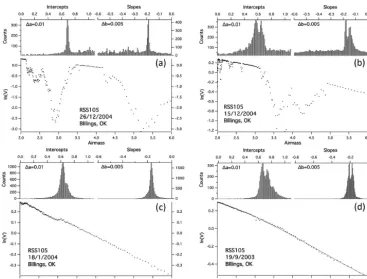
Figure 1. Four cases that illustrate how slope and intercept histograms can aid in analysis of points for the extraction of the Langley plot. In (b) and (d) both the slope and intercept histograms are bimodal. In case (c) only the histogram of intercepts is bimodal. Case (a) has many outliers, but both histograms are mono-modal indicating the existence of a single Langley plot. Case (d) has no large outliers, butyvs.xis nonlinear (third-degree polynomial).
A similar process can be performed with the histogram of intercepts. The results, however, were not as good as with the histogram of slopes.
In Fig. 1a–d we show three cases in which the H-βmethod fails and one case with a large number of outliers for which H-β works correctly. The cases are shown to illustrate the usefulness of a histogram analysis in prescreening cases and possibly designing a more sophisticated method that could produce not one but several Langley plots from one set of pointsP.
In Fig. 1a there are two regions: 2≤x≤2.12, which contains 46 points, and 3.51≤x≤4.16, which contains 19 points. These two regions produced two mono-modal, nar-row histograms, implying that there are many collinear points from within two regions.
In Fig. 1b there are two regions with collinear points. How-ever, each region has a different slope, and it extrapolates to a differentα. Both histograms are bimodal. Two distinct Lan-gley lines could be produced in this case. Only one, if ei-ther, can be right. The question that one of them or both are anomalous Langley plots can be posed.
Figure 1c shows a very interesting case. The histogram of slopes is mono-modal, but the histogram of intercepts is bi-modal. The height of the second mode is less than half of the dominant mode. Two regions 2.25≤x≤3 and 3≤x≤6
have similar slopes as they produce the mono-modal his-togram of slopes. But atx=3 there is a step change. It is not possible that it was produced by a change in the opti-cal depth if one excludes the change inεresponsible for the anomalous Langley. It is possible that atx=3 something af-fected the responsivity of the instrument. In this case we will get two Langley plots that are almost parallel with different α’s.
Figure 1d depicts a case without major outliers. The points can be fairly well approximated with a third-degree poly-nomial (a thin line is depicted), which means thatτ is the second-degree polynomial of air mass. Both histograms are bimodal and rather broad. One may pose the question of whether histograms could be used to detect nonlinearity. The method proposed by Kuester et al. (2003) has the potential for detecting the nonlinearities; however, it seems that the authors did not explore this possibility.
8 The data set
(SGP) site near Billings, Oklahoma, USA (36.6044◦N,
−97.4853◦W), between May 2003 and December 2008. The data set analyzed covers the period from 5 October 2003 to 30 March 2006, i.e., 1055 days. We removed many overcast days and several corrupted files that, together with the in-strument down times, reduced the data set to 1023 morning or afternoon setsP = {(yi, xi):2≤xi≤6}. Data from one
pixel, out of 1024, at approximatelyλ=500 nm are used in this analysis.
The RSS was lamp calibrated every 2–3 weeks with cali-brators that had lamp calibrations traceable to a NIST stan-dard. The values of V were normalized by the responsiv-ity obtained from each lamp calibration and interpolated be-tween the calibration days. This reduced trends in V0 due
to the instrumental instability caused by optical elements ag-ing, diffuser degradation, and CCD response changes. Never-theless, the RSS displayed quasi-periodic instabilities due to what we later discovered was an outgassing problem that led to a deposition of a thin film on the cooled windowless CCD. This resulted in a wavelength- and time-dependent etalon ef-fect that afef-fected the CCD’s response. Lamp calibrations mit-igated the effect but did not remove it from the data com-pletely.
9 Comparison of methods
In the previous sections we described 11 methods to iden-tify a Langley plot. In this section we compare them at four different values of rmsmax =0.010,0.008,0.006, and 0.004
using one data set. First we look at some statistical param-eters concerning 1α between each two methods, and then we look at calibration constant time series derived from each method.
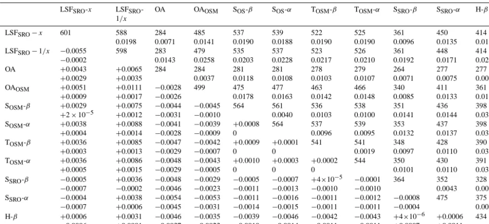
In Table 1 we collected information on the number of Lan-gley plots for each method (in the diagonal of the table) and the number of common Langley plots between the two meth-ods (above the diagonal). Then we included some statistical parameters on 1αbetween each of the two methods; there are 55 combinations. Above the diagonal is the standard de-viation of1α, and below the diagonal mean and median of 1α. The order of subtraction in1αis as follows:αfor the method from the row minusαfor the method from the col-umn.
The LSF methods produce the largest number of Lang-ley plots (601 and 598) while the OA the lowest (284). The OA’sα’s are larger than any other method by 0.0026–0.0065, which translates to 0.26–0.65 % inV0. For most cases
me-dians of 1αare 5 to 10 times smaller than means of 1α. This is because the main contribution to differences 1α among methods comes from the tails of1αdistributions. In other words, outliers are responsible for the main differences among the methods; however, some biases exist among them. A large median1αindicates that the bias between the meth-ods given by a mean is real and does not apply only to the
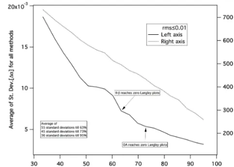
Figure 2. The average over all methods of standard deviations of
1αas a function of number of points in a Langley plot.
outliers. In Fig. 2 we demonstrate the effect of the number of outliers on the differences among the methods. The average of the standard deviations of1αfor all methods is plotted against the percentage of points retained by Langley meth-ods. When Langley plots have no more than 10 % outliers, the standard deviations between the methods are an order of magnitude smaller than when the number of outliers is up to 67 %. This implies that the main differences between meth-ods are due to different handling of outliers by each method, and the outcome is more method dependent when the Lan-gley plot consists of a smaller number of points. Also, we plotted the number of Langley plots vs. the number of points remaining in the Langley plot for the LSFSRO−xmethod to
demonstrate how strongly the number of available Langleys diminishes with the number of outliers for the site in Okla-homa.
Also, we plotted the number of Langley plots vs. the number of points remaining in the Langley plot for the LSFSRO−x method.
The Theil and Siegel methods (TOSM-β, TOSM-α, SOSM-β,
SOSM-α)produce very similar results with some of the lowest
means and medians of1α. In some cases medians are zero. We could not discern a difference between the “intercept-first methods” (TOSM-α, SOSM-α)and the “slope-first methods”
(TOSM-β, SOSM-β).
LSFSRO−xyields largerαthan LSFSRO−1/x(by 0.0055).
For rmsmax=0.010,0.008, and 0.004, it is 0.0083, 0.0065,
and 0.0039, respectively. The standard deviation of 0.0198 is not exceptionally large or small in comparison with other methods.
The Siegel methods with sequential removal of outliers (SSRO-β, SSRO-α) yield significantly different numbers of
Table 1. The comparison among 11 Langley methods for rms≤0.006. Number of successful Langley plots is on diagonal. Above the diagonal the number of common Langley plots for two methods and a standard deviation of differences1α. Below the diagonal the mean and median of1α. The order of subtraction in1αis as follows:αfor the method from row minusαfor the method from the column.
LSFSRO-x LSFSRO -1/x
OA OAOSM SOS-β SOS-α TOSM-β TOSM-α SSRO-β SSRO-α H-β
LSFSRO−x 601 588 0.0198 284 0.0071 485 0.0141 537 0.0190 539 0.0188 522 0.0190 525 0.0190 361 0.0096 450 0.0135 414 0.0164 LSFSRO−1/x −0.0055
−0.0002 598 283 0.0143 479 0.0258 535 0.0203 537 0.0228 523 0.0217 526 0.0210 361 0.0192 448 0.0171 414 0.0201 OA +0.0043
+0.0029 +0.0065 +0.0035 284 284 0.0037 281 0.0118 281 0.0108 278 0.0103 279 0.0107 264 0.0071 277 0.0075 277 0.0077 OAOSM +0.0051
+0.0009 +0.0111 +0.0017 −0.0028 −0.0026 499 475 0.0178 477 0.0163 463 0.0142 466 0.0148 340 0.0085 411 0.0133 361 0.0113 SOSM-β +0.0029
+2×10⁻⁵
+0.0075 +0.0012 −0.0044 −0.0031 −0.0045 −0.0010 564 561 0.0040 536 0.0103 538 0.0100 351 0.0141 436 0.0144 398 0.0373 SOSM-α +0.0038
+0.0004 +0.0088 +0.0014 −0.0041 −0.0028 −0.0039 −0.0009 +0.0008 0 564 537 0.0096 539 0.0095 353 0.0132 437 0.0137 398 0.0372 TOSM-β +0.0036
+0.0003 +0.0085 +0.0013 −0.0047 −0.0029 −0.0042 −0.0007
+0.0009 0
+0.0001 0 541 541 0.0019 348 0.0097 428 0.0110 390 0.0369 TOSM-α +0.0036
+0.0005 +0.0086 +0.0015 −0.0048 −0.0029 −0.0043 −0.0005
+0.0010 0
+0.0003 0
+0.0002 0 544 350 0.0101 430 0.0110 391 0.0367 SSRO-β −0.0005
−0.0007 +0.0036 −0.0002 −0.0048 −0.0046 −0.0029 −0.0023 −0.0005 −0.0011 −0.0007 −0.0013
+4×10⁻⁵
−0.0010 −0.0001 −0.0010 364 352 0.0043 328 0.0061 SSRO-α −0.0004
−0.0007 +0.0038 +0.0006 −0.0054 −0.0045 −0.0053 −0.0031 −0.0011 −0.0014 −0.0016 −0.0015 −0.0011 −0.0011 −0.0012 −0.0011 −0.0008 −0.0004 475 375 0.0064 H-β +0.0006
−0.0006 +0.0031 +0.0001 −0.0046 −0.0037 −0.0035 −0.0023 −0.0039 −0.0010 −0.0046 −0.0014 −0.0042 −0.0011 −0.0043 −0.0011
+4×10⁻⁶
+0.0007
+0.0006
+0.0011 434
The results for the histogram method H-βdo not indicate anything extraordinary. Its results are most similar to results produced by Siegel methods and LSFSRO−x.
The outlier sorting method when applied to OA increases the number of Langley plots by 75 %. On the common set of data the OAOSMproduces smallerα’s (by 0.0028). This
is the opposite effect of OSM compared to NPF methods (see Sect. 5). The extra Langleys produced by the OAOSM
method do not necessarily indicate an improvement. Many of them are large outliers in the time series. We conclude that the OA, if it errs, it errs on being conservative: it has a fairly large missed detection rate (rejecting data sets with vi-able Langley plots), and at the same time the ones that are detected sometimes could be improved by a removal of few extra outliers.
When evaluating individual plots, and we looked at almost all 11×1023 of them, we found for each method cases when it went astray. There were cases of missed detection and false detection when judged by eye. However, we cannot quantify which of the algorithms has the most favorable missed and false detection rates. Out of all algorithms used, only OA deals explicitly with curvature. This perhaps might be a chief reason why it produces significantly fewer Langleys, which leads to a smaller number of large outliers in the time series. The comparison of calibration constants that can be de-rived fromα’s obtained by each method gives us additional insight about each method as well as a strategy one should use when generating the calibration constants. We compare the behavior of time series of derived calibration constants αcc(d), whered indicates each day from 5 October 2003 to
30 March 2006. Theαcc(d)’s are obtained from the time
se-ries ofα(dj)independently for each Langley method, where djdenotes days at which Langleys were obtained. Theαcc(d)
might be considered “the best” estimate of the calibration constant for a given day, “the best” in the sense of the method that we use to remove outliers, interpolate and smooth the se-riesα(dj).
The method consists of a moving median window of width dmeddays that removes outliers and interpolates, which is
fol-lowed by a moving boxcar filter. For each dayd the median is calculated fromdmednumber ofα(dj)values:dmed/2
val-ues fordj≤danddmed/2 values ford<dj. Then the
1055-long seriesαcc(d)is smoothed with a boxcar filter ofdsmth
days. By trial and error we decided ondmed=30 days and
dsmth=25 days.
Prior to applying the method described above, the values of αare corrected for Earth–Sun distance a by a substitu-tionα← −α+2ln(a), whereais in astronomical units. The Earth–Sun distance is calculated with the ephemeris program published by Michalsky (1988).
One of the methods of time-series smoothing ofV0’s to
obtain the absolute calibration constants of a sun photometer (MFRSR) was validated against calibrations at Mauna Loa by Michalsky and LeBaron (2013). The discrepancy between the time-series smoothing and Mauna Loa calibration con-stants in terms ofV0’s was always smaller than 0.6 %. This
Figure 3. Calibration constant curves for all 11 methods (rms < 0.006) and individual interceptsαfor OA and H-βmethods.
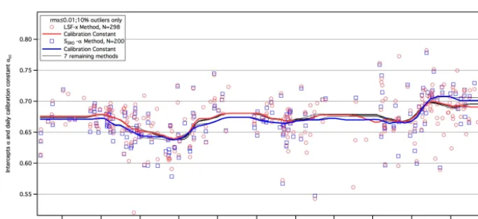
Figure 4. Calibration constants curves for nine methods (rms < 0.01) from Langley plots with no more than 10 % outliers and individual interceptsα’s for LSFSRO−xand SSRO-αmethods. (The OA and H-βresults did not pass the filter of 10 % outliers only.)
In Fig. 3 we show all 11αcc(d)curves and individual
in-tercepts α’s from OA and H-β methods for rms≤0.006. In the course of 1055 days the RSS’s calibration constants vary within ±3.5 % (in terms ofV0) band. All methods follow these changes; however, there are differences among them. Statistically, the differences are±1.4 for 95 % of days from the calibration constant curve that is the average of all 11 curves. For other values of rmsmax0.010, 0.008, and 0.004,
the differences are ±1.6, ±1.45, and±1.4 %, respectively. The effect of the maximum rms on the differences between the αcc(d)curves is not very dramatic. This is because the
parameter dmed=30 days of the median filter is relatively
large.
In Fig. 4 we show nine calibration constant curves and in-terceptsα’s for LSFSRO−x and SSRO-αmethods for rms≤
0.010. In this case we usedα’s from Langley plots that had no more than 10 % outliers. The OA and H-β results did not pass the filter of 10 % outliers only. The differences be-tween the calibration constant curves are±0.8 %. For 40, 30, and 20 % outliers, the calibration constant curves are within
±1.2,±0.9, and±0.87 % bands, respectively. So, the effect
of number of outliers removed to obtain a Langley plot has a larger effect on the spread among the methods than the effect of rmsmax.
We note that the OA and H-β calibration constant curves from Fig. 3 are marginally within the band defined by the curves in Fig. 4.
The majority of points in Fig. 4 are outliers, and they are defined by Langley plots with 90 % or more points. By the criterion rms≤0.01 the points are collinear. Nevertheless, they are off and some by more than±5 % (in terms ofV0). In
our opinion, the majority of the outliers are cases of anoma-lous Langley plots. The topic of anomaanoma-lous Langley plots will be pursued in another paper.
10 Conclusions and summary
We developed two methods to terminate the non-parametric methods in order to determine the existence of the Langley plot: the outlier sorting method (OSM) that was applied to two Theil (1950) and two Siegel (1982) methods, and a new non-parametric method of sequential removal of outliers (SRO) was applied to two Siegel methods resulting in two new iterative Siegel methods.
We found that analysis of histograms of slopes and in-tercepts can be an excellent tool to prescreen a data set for Langley-plot viability. The histogram of slopes was used to generate Langley plots that produce lines defined by a small number of points. The histogram method offers a possibility to extract Langley plots when outliers dominate and to find all subsets of collinear points.
The OA method turned out to be robust though conser-vative. It identifies the lowest number of Langley plots. It produces intercepts slightly larger than all other methods.
The Siegel (1982) and Theil (1950) methods with OSM produce very similar results. The two least square methods yield the largest number of Langley plots, with expected bias between them.
The largest differences among methods are on Langley plot cases that turn out to be outliers in terms of the calibra-tion constant curve. Predominantly these are the cases that produce Langley plots but with a small number of points. In cases that are close to the calibration constant curve the dif-ferences are small, but there are systematic biases.
We have no way of determining which of the methods pro-duces results closest to the truth. In fact, the answer may de-pend on the data set. When the number of outliers in a Lang-ley plot is small, all methods tend to produce similar results. The metrics used to define the Langley plot was rms of residuals. The effect of the value of rms, whether it was 0.10 or 0.06, had no great impact on the calibration constant curves: all methods produced calibration constant curves within a band between±1.4 and±1.6 % for 95 % of days. It is the number of outliers in the data set that has a greater im-pact. The calibration curves generated using a smaller num-ber of Langley plots with each Langley defined by a larger number of points produce calibration constant curves that are less dependent on the method. For instance when Langley plots retain 80 % of the points all calibration constant curves are within±0.9 % band for 95 % of days.
The outliers from the calibration constant curves are pre-dominantly caused by anomalous Langley plots when the op-tical depth has a hyperbolic component as a function of air mass. This effect cannot be detected from the data set, and no Langley plot method can determine if this hyperbolic change with air mass is occurring. This effect at difficult sites like the SGP ARM site in Oklahoma sets the ultimate limit of accuracy of in situ calibrated sun photometers.
Acknowledgements. We want to express our gratitude to Robert
Evans of NOAA, Boulder, Colorado for providing the G.M.B. Dob-son 1958 report; Bruce Forgan of Bureau of Meteorology, Melbourne, Australia, for providing information on his approach to Langleys; Alberto Redondas of Izaña Atmospheric Research Center, Tenerife, Spain, for providing information on Langleys in the Brewer network; Jim Schlemmer of ASRC, SUNY at Albany, NY, for running the OA Langley method on RSS data. The final shape of the paper owes much to constructive input of two anonymous reviewers.
Edited by: A. Kokhanovsky
References
Augustine, J. A., Cornwall, C. R., Hodges, G. B., Long, C. N., Med-ina, C. I., and DeLuisi, J. J.: An automated method of MFRSR calibration for aerosol optical depth analysis with application to an Asian dust outbreak over the United States, J. Appl. Meteo-rol., 42, 266–278, 2003.
Birknes D. and Dodge Y.: Alternative Methods of Regression, Wiley-Interscience, 240 pp., ISBN978-0-471-56881-0, 1993. Cachorro, V. E., Romero, P. M., Toledano, C., Cuevas, E., and
de Frutos, A. M.: The fictitious diurnal cycle of aerosol opti-cal depth: A new approach for “in situ” opti-calibration and cor-rection of AOD data series, Geophys. Res. Lett., 31, L12106, doi:10.1029/2004GL019651, 2004.
Cachorro, V. E., Toledano, C., Berjón, A., de Frutos, A. M., Torres, B., Sorribas, M., and Laulainen, N. S.: An “in situ” calibration correction procedure (KCICLO) based on AOD diurnal cycle: Application to AERONET–El Arenosillo (Spain) AOD data series, J. Geophys. Res., 113, D12205, doi:10.1029/2007JD009673, 2008.
Campanelli, M., Nakajima, T., and Olivieri, B.: Determination of the solar calibration constant for a sun-sky radiometer: Proposal of an in situ procedure, Appl. Optics, 43, 651–659, 2004. Forgan, B.: Practical sun spectral radiometer calibration methods,
International Pyrheliometer Comparison, PMOD-World Radia-tion Center, Davos, Switzerland, 2000.
Dobson, G. M. B. and Normand, C.: Determination of Constants Used in the Calculation of the Amount of Ozone from Spec-trophotometer Measurements and the Accuracy of the Results, International Ozone Commission (I. A.M.A.P.), October, 1958. Harrison, L. and Michalsky, J.: Objective algorithms for the retrieval
of optical depths from ground based measurements, Appl. Op-tics, 33, 5126–5132, 1994.
Harrison, L. Michalsky, J., and Berndt, J.: Automated Multi-Filter Rotating Shadowband Radiometer: An Instrument for Optical Depth and Radiation Measurements, Appl. Optics, 33, 5118– 5125, 1994.
Harrison, L., Beauharnois, M., Berndt, J., Kiedron, P., Michalsky, J., and Min, Q.: The rotating shadowband spectroradiometer (RSS) at SGP, Geophys. Res. Lett., 26, 1715–1718, 1999.
Herman, B. M., Box, M. A., Reagan, J. A., and Evans, C. M.: Al-ternate approach to the analysis of solar photometer data, Appl. Optics, 20, 2925–2928, 1981.
Ito, M., Uesato, I., Noto, Y., Ijima, O., Shimidzu, S., Takita, M., Shi-modaira, H., and Ishitsuka, H.: Absolute Calibration for Brewer Spectrophotometers and Total Ozone/UV Radiation at Norikura on the Northern Japanese Alps, Journal of the Aerological Ob-servatory, 72, 45–55, 2014.
Jaeckel, L.: Estimating the regression coefficients by minimizing the dispersion of residuals, Ann. Mat. Stat., 43, 1449–1458, 1972.
Kasten, F.: A new table and approximation formula for the relative optical air mass, Arch. Meteor. Geophy. B., Ser. B, 14, 206–223, 1965.
Kendall, M. G.: A new measure of rank correlation, Biometrika, 30, 81–93, 1938.
Kuester, M. C., Thome, K. J., and Reagan, J. A.: Automated statisti-cal approach to Langley evaluation for a solar radiometer, Appl. Optics, 42, 4914–4921, 2003.
Kiedron, P. W., Michalsky, J. J., Berndt, J. L., and Harrison L. C.: Comparison of spectral irradiance standards used to calibrate shortwave radiometers and spectroradiometers, Appl. Optics, 38, 2432–2439, 1999.
Long, C. N. and Ackerman, T. P.: Identification of clear skies from broadband pyranometer measurements and calculation of down-welling shortwave cloud effects, J. Geophys. Res.-Atmos., 105, 15609–15626, 2000.
Marenco, F.: On Langley plots in the presence of a systematic diur-nal aerosol cycle centered at noon: A comment on recently pro-posed methodologies, J. Geophys. Res.-Atmos., 112, D06205, doi:10.1029/2006JD007248, 2007.
Michalsky, J. J.: The Astronomical Almanac’s algorithm for ap-proximate solar position (1950–2050), Sol. Energy, 40, 227–235, 1988.
Michalsky, J. and LeBaron, B.: Fifteen-year aerosol optical depth climatology for Salt Lake City, J. Geophys. Res-Atmos., 118, 3271–3277, doi:10.1002/jgrd.50329, 2013.
Mlawer, E. J., Brown, P. D., Clough, S. A., Harrison, L. C., Michal-sky, J. J., Kiedron, P. W., and Shippert, T.: Comparison of spectral direct and diffuse solar irradiance measurements and calculations for cloud-free conditions, Geophys. Res. Lett., 27, 2653–2656, 2000.
Nieke, J., Pflug, B. G., and Zimmermann, G.: An aureole-corrected Langley-plot developed for the calibration of HiRES grating spectrometers, J. Atmos. Sol-Terr. Phy., 61, 739–744, 1999. Redondas, A.: RBCC-E ozone absolute calibration, langley
regres-sion method, The Ninth Biennial WMO Consultation on Brewer Ozone and UV Spectrophotometer Operation, Calibration and Data Reporting, 69 pp., 2005.
Schmid, B. and Wehrli, C.: Comparison of Sun photometer cali-bration by use of the Langley technique and the standard lamp, Appl. Optics, 34, 4500–4512, doi:10.1364/AO.34.004500, 1995. Shaw, G. E.: Error analysis of multi-wavelength Sun photometry”,
Pure Appl. Geophys. 114, 1–14, 1976.
Siegel, A. F.: Robust regression using repeated medians, Biometrika, 69, 242–244, doi:10.1093/biomet/69.1.242, 1982. Tanaka, M., Nakajima, T., and Shiobara, M.: Calibration of a
sun-photometer by simultaneous measurements of direct-solar and circumsolar radiations, Appl. Optics, 25, 1170–1176, 1986. Theil, H.: A rank-invariant method of linear and polynomial
regres-sion analysis. I, II, III, Nederl. Akad. Wetensch., Proc., 53, 386– 392, 521–525, 1397–1412, 1950.