Nonlin. Processes Geophys., 17, 361–369, 2010 www.nonlin-processes-geophys.net/17/361/2010/ doi:10.5194/npg-17-361-2010
© Author(s) 2010. CC Attribution 3.0 License.
Nonlinear Processes
in Geophysics
Image-model coupling: application to an ionospheric storm
N. D. Smith1,*, D. Pokhotelov2, C. N. Mitchell2, and C. J. Budd1
1Department of Mathematical Sciences, University of Bath, Bath, BA2 7AY, UK
2Department of Electronic and Electrical Engineering, University of Bath, Bath, BA2 7AY, UK
*Completed while with the Department of Electronic and Electrical Engineering, University of Bath, Bath, BA2 7AY, UK Received: 7 October 2008 – Revised: 16 July 2010 – Accepted: 26 July 2010 – Published: 20 August 2010
Abstract. Techniques such as tomographic reconstruction may be used to provide images of electron content in the ionosphere. Models are also available which attempt to de-scribe the dominant physical processes operating in the iono-sphere, or the statistical relationships between ionospheric variables. It is sensible to try and couple model output to tomographic images with the aim of inferring the values of driver variables which best replicate some description of electron content imaged in the ionosphere, according to some criterion. This is a challenging task. The following describes an attempt to couple an ionospheric model to a tomographic reconstruction of the geomagnetic storm of 20 November 2003, along a latitudal line segment above north America. A simple model was chosen to reduce the number of input drivers that were varied. The investigation illustrates some of the issues involved in image-model coupling. The ability to make scientific deductions depends on the accuracy of the assumptions in the ionospheric model and the accuracy of the tomographic reconstruction. An ensemble technique was used to help assess confidence in the reconstruction.
1 Introduction
The ionosphere is a complex system with multiple processes operating at different scales. Understanding these processes is of scientific value, and has practical benefit in applications such as communication and navigation. In recent years, dif-ferent empirical and physical models have been developed to explain how the ionosphere, typically in terms of its plasma content, responds to external stimuli or drivers. The map-ping from the space of driver variables to the space of vari-ables describing the ionosphere is expected to be nonlinear, especially for an extreme event such as a geomagnetic storm.
Correspondence to: N. D. Smith
(n.smith@bath.ac.uk)
Hence it would be interesting to study the sensitivity of the response to different drivers. This may give further insight into which processes dominate under different conditions. Also, those drivers to which the response is most sensitive may require more accurate or more frequent measurement in future.
One means of investigating the ionosphere, including sen-sitivity of its response to drivers, is via image-model cou-pling. This is a challenging task. This paper describes some relevant issues, and presents techniques which may be use-ful for future developments in image-model coupling. Im-ages of electron density may be obtained, for example, by tomographic reconstruction techniques (Bust and Mitchell, 2008; Pryse et al., 1998). Once a sequence of images is ob-tained for an ionospheric event, an ionospheric model is then selected, its drivers varied, and the closeness of match be-tween the model output and image sequence calculated. The shape of the matching function gives an indication of sen-sitivity, for the particular event and subject to the accuracy of the ionospheric model. This approach may also encour-age a better appreciation of the limitations and assumptions in the ionospheric model being used. A framework for de-scribing image-model coupling in terms of communication along a discrete channel is presented in (Smith et al., 2009). This paper describes a simple application of these ideas to an extreme event, the geomagnetic storm of 20 November 2003. The matching function is very simple and many of the statistical conditional dependencies between data at suc-cessive timesteps are ignored. The features and matching function are described briefly in Sect. 2. The tomographic reconstruction is presented in Sect. 3, and the analysis for an ionospheric model in Sect. 4. Some discussion and conclu-sions follow in Sects. 5 and 6, respectively.
362 N. D. Smith et al.: Image-model coupling: application to an ionospheric storm
00 03 06 09 12 15 18 21
−500 −400 −300 −200 −100 0 Dst (nT) UT
00 03 06 09 12 15 18 21
−40 −20 0 20 Bz (nT) GSE UT
00−02 03−05 06−08 09−11 12−14 15−17 18−20 21−23
0 100 200 300 400 Ap UT
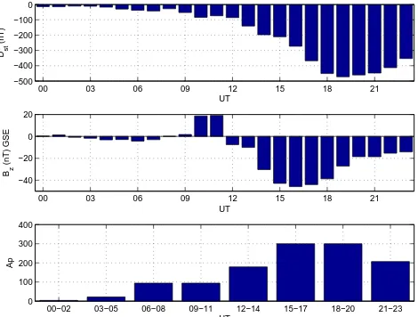
Fig. 1. Hourly measurements for Dst and Bz, and three-hourly mea-surements for Ap (see OMNIWeb, access: July 2010 and the Ac-knowledgments).
as expected, occurs during a southward orientation of the IMF (values for the IMF Bz component are also available at a higher sampling rate than hourly). In addition, theF10.7 value for the day was 171.0 (see OMNIWeb, access: July 2010, see also the Acknowledgments).
2 Calculating features and optimising the match
It is often convenient to calculate ionospheric data at a dis-crete set of points on a grid which is uniform in altitude, and geographic latitude and longitude coordinates. The grid points are represented as blackened circles in the sketch of a slice of constant geographic latitude in Fig. 2. Assume the grid is indexed by(l,m,n) wherel∈ [1,L] is an index for altitude above the Earth’s surface,m∈ [1,M]for geographic latitude andn∈ [1,N]for geographic longitude. The altitude of a grid point ishg(l,m,n)and the electron density at that point isNg(l,m,n). The grid points are used to define cells in the manner of Fig. 2 where grid points are cell centres; the exceptions are the “half-cells” at the top and foot of the cell structure. Hence cell centreshc(l,m,n)are defined with the following altitudes. For alll,m,
hc(l,m,n)= 3
4hg(L,m,n)+ 1
4hg(L−1,m,n) if l=L hg(l,m,n) if 1< l < L 3
4hg(1,m,n)+ 1
4hg(2,m,n) if l=1 ,
(1) where it is assumed L>1. The electron densities at the cell centres are defined such that Nc(l,m,n)=Ng(l,m,n),
∀l,m,n. Electron density is assumed uniform in a cell. The cells are contiguous, and each cell has a vertical length
8 N.D. Smith et al.: Image-model coupling: application to an ionospheric storm
Korn, G. and Korn, T.: Mathematical Handbook for Scientists and Engineers: Definitions, Theorems, and Formulas for Reference and Review, McGraw-Hill,Inc., second, enlarged and revised edn., New York, 1968.
Mannucci, A., Tsurutani, B., Iijima, B., Komjathy, A., Wilson, B., Pi, X., Sparks, L., Hajj, G., Mandrake, L., Gonzalez, W., Kozyra, J., Yumoto, K., Swisdak, M., Huba, J., and Skoug, R.: Hemi-spheric Daytime IonoHemi-spheric Response To Intense Solar Wind Forcing, in: Inner Magnetosphere Interactions: New Perspec-tives from Imaging, edited by Burch, J., Schulz, M., and Spence, H., vol. 159 of Geophysical Monograph Series, pp. 261–275, American Geophysical Union, Washington, DC, 2005.
Mitchell, C. and Spencer, P.: A three-dimensional time-dependent algorithm for ionospheric imaging using GPS, Ann. Geophys.-Italy, 46, 687–696, 2003.
OMNIWeb: Space Physics Data Facility, NASA/Goddard Space Flight Center, http://omniweb.gsfc.nasa.gov, access: July 2010. Powell, M.: A view of algorithms for optimization without
deriva-tives, Mathematics TODAY, 43, 170–174, 2007.
Pryse, S., Kersley, L., Mitchell, C., Spencer, P., and Williams, M.: A comparison of reconstruction techniques used in ionospheric tomography, Radio Sci., 33, 1767–1779, 1998.
SAMI2: The SAMI2 Open Source Project, Naval Research Lab-oratory, http://wwwppd.nrl.navy.mil/sami2-OSP/index.html, ac-cess: November 2007.
SAMI3: NRL Ionosphere Model: SAMI3,
http://www.nrl.navy.mil/content.php?P=04REVIEW105, access: September 2008.
Smith, N., Mitchell, C., and Budd, C.: Image-model coupling: a simple information theoretic perspective for image sequences, Nonlin. Proc. Geophys., 16, 197–210, 2009.
SOPAC website ref.: Scripps Orbit and Permanent Array Center (SOPAC), http://sopac.ucsd.edu.
Spencer, P. and Mitchell, C.: Imaging of fast moving electron-density structures in the polar cap, Ann. Geophys.-Italy, 50, 427– 434, 2007.
The MathWorks: http://www.mathworks.com, access: November 2009.
Tsurutani, B., Verkhoglyadova, O., Mannucci, A., Araki, T., Sato, A., Tsuda, T., and Yumoto, K.: Oxygen ion uplift and satel-lite drag effects during the 30 October 2003 daytime superfoun-tain event, Ann. Geophys.-Germany, 25, 569–574, available at: http://www.ann-geophys.net/25/569/2007/, 2007.
00 03 06 09 12 15 18 21
−500 −400 −300 −200 −100 0 Dst (nT) UT
00 03 06 09 12 15 18 21
−40 −20 0 20 Bz (nT) GSE UT
00−02 03−05 06−08 09−11 12−14 15−17 18−20 21−23
0 100 200 300 400 Ap UT
Fig. 31. Hourly measurements forDst andBz, and three-hourly measurements forAp(see (OMNIWeb, access: July 2010) and the Acknowledgments). grid point cell longitude direction direction radial
Fig. 32. Sketch showing how grid points are related to cells.
Table 31. Key driver variables for SAMI2 optimised against the ensemble mean from MIDAS, along the latitudinal line segment, for the VTEC feature space, and for different time windows during 20 November 2003.
time window optimal parameters
s (UT) F10.7 Ap V /ms−
1
1 1200h - 1400h 50.0 0 225.0 2 1500h - 1700h 50.0 80 225.0 3 1800h - 2000h 300.0 80 100.0 4 2100h - 2300h 250.0 0 100.0 Fig. 2. Sketch showing how grid points are related to cells.
d(l,m,n). The electron content of the ionosphere may be summarised using vertical total electron content (VTEC) or mean ionospheric height (i.e. the height of the centre of mass of the electrons). In the following experiments, VTEC is used.
VTEC(m,n)= L X
l=1
d(l,m,n)Nc(l,m,n). (2) The 2-D map may then be assembled into a column vector, for example the (MN×1) feature vector,
z=(VTEC(1,1),...VTEC(M,N ))>. (3) Assume an image sequencez(1,l)=(z1,...,zl)obtained by
tomographic reconstruction, and outputz0(1,l)=(z01,...,z0l) obtained by a physical model. Then, giving equal weight to each cell, the unweighted sum square error between the two sequences is,
f z(1,l),z0(1,l)= l X
t=1
zt−z0t>
zt−z0t
. (4)
Given competing model outputs, the output of closest match is,
ˆ
z0(1,l)=argz0(1,l)minf z(1,l),z0(1,l)
. (5)
This minimisation is the least sum square error estimate. In the following experiments, each model output sequence was obtained by fixing a subset of driver variables at a vector valueu. Hence,
ˆ
u=arguminf (z(1,l),u), (6)
assuming u7→z0(1,l) is injective. In effect, the physical model is being used to “decode” the values of driver vari-ables, assuming the tomographic reconstruction is correct and true. As described more fully in (Smith et al., 2009),
ˆ
N. D. Smith et al.: Image-model coupling: application to an ionospheric storm 363 3 Tomographic reconstruction using MIDAS
MIDAS (“Multi-Instrument Data Analysis System”) ver-sion 3 (see Appendix A, and a previous verver-sion of the soft-ware described in Mitchell and Spencer, 2003) was used to tomographically reconstruct electron densities above north America using the total electron content (or slant TEC) along raypaths between satellites and IGS1receiver stations. The reconstruction was conducted hourly from 12:00 UT to 23:00 UT inclusive for 20 November 2003, and over a (39×6×7) structure of grid points (this included altitudes at 90 km, and from 100 km to 1580 km inclusive at 40 km in-tervals; geographic latitudes from 25◦N to 50◦N inclusive at 5◦intervals; geographic longitudes from 130◦W to 70◦W inclusive at 10◦ intervals). Two sets of data were used; the
training set collected from 89 receivers and the evaluation set collected from 82 receivers. The two sets of receivers did not share members, and the receivers were fairly evenly selected from those IGS1receivers available. Locations are detailed in Fig. 3.
The receiver data was first sampled at 5 min intervals over the entire day. At 12:00 UT, the ionosphere was assumed static for 20 min from 11:50 UT to 12:10 UT (5 frames of data). An estimate for electron content was obtained by seek-ing those electron densities at each point in the grid which minimised the regularised sum square error of slant TEC as measured by each receiver/transmitter pair. For each pair, the unknown offset relating the phase difference between the two channels of the dual-frequency receiver and slant TEC was also assumed fixed across the 20 min window, and esti-mated to minimise the regularised sum square error of slant TEC. The regularised least sum square error problem can be solved by an appropriate quadratic programming solver (here MATLAB2’s quadprog function was used, explicitly enforc-ing nonnegativity constraints for electron densities, with a suitable tolerance and a limit in the number of iterations, and a fixed nonzero initialisation). The optimisation was then re-peated hourly until 23:00 UT inclusive.
Details of the optimisation and regularisation are given briefly in Appendix A. Regularisation involved smoothing the zeroth, first and second-order derivatives of the electron densities in four horizontal spatial directions towards those in the International Reference Ionosphere, 1995 (IRI-95) (Bil-itza, 1997); the IRI model was also used in a different though similar approach in Bhuyan and Bhuyan (2007). The amount of regularisation was governed by regularisation parame-ters λi3∈ {0,0.0001,0.001,0.01,0.1,1,10,100} for second-order derivatives, andλik∈ {0,0.0001,0.01,1,100}, k∈ {1,2}
for zeroth and first-order derivatives, where larger values of λik,k∈ {1,2,3}indicate greater smoothing and i is sim-ply an index for the model being trained. Hence a tomo-graphic reconstruction was obtained for each permutation of
1http://igscb.jpl.nasa.gov
2The MathWorks, http://www.mathworks.com
N.D. Smith et al.: Image-model coupling: application to an ionospheric storm 9
Fig. 33. Locations of IGS receivers used in training (blue “ + ”) and evaluation (red “ x ”); the tomographic reconstruction is delimited by the black box, and the comparison with SAMI2 output is along the central magenta line.
0 200 400 600 800 1000 1200 1400 1600
−0.6 −0.5 −0.4 −0.3 −0.2 −0.1 0 0.1 0.2 0.3
electron density (x 10
+
1
1 m
−
3)
altitude (km)
Fig. 34. Vertical basis functions used for the tomographic recon-structions with MIDAS.
Fig. 3. Locations of IGS1receivers used in training (blue “ + ”) and evaluation (red “ x ”); the tomographic reconstruction is delimited by the black box, and the comparison with SAMI2 output is along the central magenta line.
(λi1,λi2,λi3)except the unregularised solution (i.e.λik=0,∀k). The ensemble of 199 members was reduced to 185 members by excluding those which contained electron densities less than−1×10⁹electrons/m3(most probably the nonnegativ-ity constraints were violated due to numerical limitations in the constrained optimiser). For each member of the new en-semble, the sum square error of slant TEC for the evaluation set was calculated (again assuming the ionosphere was fixed over a 20 min window, and that the unknown offsets were also fixed over the time window and were estimated to min-imise the sum square error on the evaluation set). The evalu-ation performance was used in a posterior weighting scheme. The candidate reconstruction for each hour was calculated as the ensemble mean, with confidence provided by the ensem-ble variance (see Appendix A for further details). However the arithmetic mean of posterior weights was not calculated across all 12 hourly timesteps, but only 9 hourly timesteps. The scaled likelihoods at each timestep were very small and were forced to zero when precision was lost. All scaled like-lihoods were set to zero at 18:00, 20:00, and 21:00 UT, so posteriors could not be calculated at those timesteps, or used in calculating the arithmetic mean of posterior weights. At other timesteps, between 1 and 143 (inclusive) members of the ensemble yielded nonzero likelihood and hence nonzero member posterior. The thresholding of member posteriors to zero due to loss in precision is not regarded as problematic, since it may be interpreted as a means of increasing robust-ness.
364 N. D. Smith et al.: Image-model coupling: application to an ionospheric storm
0 200 400 600 800 1000 1200 1400 1600
−0.6 −0.5 −0.4 −0.3 −0.2 −0.1 0 0.1 0.2 0.3
electron density (x 10
+11
m
−3
)
altitude (km)
Fig. 4. Vertical basis functions used for the tomographic reconstruc-tions with MIDAS.
structure, only (n×6×7) basis function coefficients were estimated, wheren is the number of basis functions in the limited set (Spencer and Mitchell, 2007). The basis functions used were thosenleft singular vectors with largest singular values, calculated from data extracted from IRI-95 (above the reconstruction region, eight times per day for four days during the year 1995).
In the following experiments, we chosen=2. The ver-tical basis functions are plotted in Fig. 4. Verver-tical profiles were therefore restricted to linear combinations of the basis functions. Admittedly, the basis functions are restrictive and should ideally be optimised dynamically from hour to hour using independent data. However this would further compli-cate the optimisation problem. For simplicity, the fixed set of vertical basis functions detailed above were always used, and the inability to model high electron densities in the topside, and small-scale features elsewhere, acknowledged.
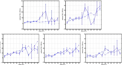
For a latitudinal line at 35◦N between 120◦W to 80◦W inclusive, the ensemble average VTEC is plotted in Fig. 5 at each 10◦spacing, hourly from 12:00 UT to 23:00 UT
inclu-sive, as a full line. Error bars corresponding to a 95% con-fidence level, albeit with a simple Gaussian error model, are also detailed. The error bars show that there is a high degree of variability across the ensemble, without even considering the extra variability expected from varying other parameters such as the number or shape of vertical basis functions, or the size of cells. The variability is in part due to the lack of constraints via horizontal basis functions, and indicates the significant challenge of such underdetermined inverse prob-lems. There is highest variability towards the eastern coast of north America. The “fixed ionosphere” assumption over 20 min may be problematic during the stormy periods.
The onset of the storm can be monitored by viewing the orientation of the IMF and the Dst index (see Fig. 1). Dif-ferent physical processes can be used to help explain the high plasma densities at midlatitudes during the geomegnetic
storm, e.g. Mannucci et al. (2005); Tsurutani et al. (2007); Foster et al. (2005). High plasma densities are probably caused by the interaction of both equatorial/low latitude pro-cesses, such as a superfountain effect, and subauroral/high latitude processes such as electron precipitation and Joule heating. Neutral winds and electric fields can lift plasma up-wards along field lines, thereby providing mechanisms to in-crease vertical total electron content at high and midlatitude locations.
4 Coupling with SAMI2
N. D. Smith et al.: Image-model coupling: application to an ionospheric storm 365
12 13 14 15 16 17 18 19 20 21 22 23
−50 0 50 100 150 200
vertical TEC (TECU)
time (UT) 12 13 14 15 16 17 18 19 20 21 22 23
−10 0 10 20 30 40 50
vertical TEC (TECU)
time (UT)
12 13 14 15 16 17 18 19 20 21 22 23
−10 0 10 20 30 40 50
vertical TEC (TECU)
time (UT) 12 13 14 15 16 17 18 19 20 21 22 23
−10 0 10 20 30 40 50
vertical TEC (TECU)
time (UT)
12 13 14 15 16 17 18 19 20 21 22 23
−10 0 10 20 30 40 50
vertical TEC (TECU)
time (UT)
Fig. 5. VTEC profiles at 35◦N between 120◦W and 80◦W inclusive (at 10◦intervals) for 20 November 2003; the full line is the en-semble mean from MIDAS with error bars at 95% confidence level; the dashed line is the optimal match with SAMI2 (1 TECU = 1×
1016electrons/m2).
E×Bdrift velocity model was used (Huba et al., 2000), pa-rameterised byV and described in Appendix B. The max-imum number of timesteps was set to 20×106. All other values which were not directly varied in the following ex-periments were set to their recommended or default settings; in particular, multiplicative factors for neutral wind speed, E×B drift velocity, neutral densities corresponding to the 7 positive ion species, and neutral temperature were all kept at unity unless otherwise stated.
In the following investigations, the key driver vari-ables varied for SAMI2 were F10.7, Ap, and V which are respectively a measure of solar radiation at 10.7 cm wavelength, a measure of geomagnetic activity, and the maximum E×B drift velocity for the sinusoidal drift model (indirectly an indication of electric field strength). These driver variables were varied such that F10.7∈ {50.0,100.0,150.0,200.0,250.0,300.0}, Ap∈
{0,15,80,207,400}which corresponds to Kp∈ {0,3,6,8,9}, andV∈ {100.0,200.0,225.0,300.0,375.0,450.0}ms−1. All other driver variables were kept at fixed values unless other-wise stated.
Optimisation results are detailed in Table 1 for four differ-ent time windows and the VTEC feature space, for match-ing VTEC along the latitudinal line segment. The log root mean square (RMS) error in VTEC for the 180 matches over each three hour window are plotted, in order of increasing RMS error, in Fig. 6. The plots illustrate that the statistical
significance in the optimisation is dubious, even without fac-toring in the errors in the underlying SAMI2 model. Nev-ertheless, the optimal SAMI2 matches are plotted as dashed lines in Fig. 5. SAMI2 struggles to match the high VTEC towards the eastern coast of north America. The drift veloc-ity model is very simple. The domain ofV applied in the optimisation includes values which imply velocities above the equator that are most probably physically impossible (see Appendix B). Due to dubious statistical significance, the sci-entific conclusions from the experiments are limited. Fur-thermore, the matching function is probably overly simple, the optimisation is over a coarse grid and does not involve the variation of other parameters (e.g. multiplicative factors for the neutral densities of positive ion species), and SAMI2 was run independently for each time-window, with no abil-ity to dynamically change parameters such asF10.7in time. Interestingly, Jee et al. (2005) describes a sensitivity analysis for VTEC, but each parameter was varied individually and not in combination.
5 Discussion
366 N. D. Smith et al.: Image-model coupling: application to an ionospheric storm
Table 1. Key driver variables for SAMI2 optimised against the en-semble mean from MIDAS, along the latitudinal line segment, for the VTEC feature space, and for different time windows during 20 November 2003.
time window optimal parameters
s (UT) F10.7 Ap V/ms−1
1 12:00–14:00 50.0 0 225.0
2 15:00–17:00 50.0 80 225.0
3 18:00–20:00 300.0 80 100.0
4 21:00–23:00 250.0 0 100.0
SAMI2 was designed to model equatorial and low latitude processes, rather than those high latitude processes which can have a significant effect at midlatitudes during a geo-magnetic storm. For example, SAMI2 was not designed to accurately model the physics of high latitude convection, and the simple sinusoidalE×Bdrift velocity model is most ap-plicable in equatorial regions. Furthermore, SAMI2 uses the HWM93 neutral wind model. This wind model is statisti-cal and is unlikely to adequately or accurately characterise the strong high latitude equatorward neutral winds, caused by Joule heating and electron precipitation, common dur-ing a large storm. Since the latitudinal line segment chosen for the coupling experiments is at midlatitudes where both equatorial and polar/auroral processes are likely to be influ-ential during a geomagnetic storm, SAMI2 may be trying to replicate the build-up of plasma at midlatitudes by driving an equatorial process in an unrealistic manner. In particular, the drift velocity model may be too simple. Since variation in the parameterV was used to mimic variation in electric field strength, improvements in electric field models may give bet-ter coupling results.
Ionospheric tomographic reconstruction techniques are susceptible to error (e.g. Dear and Mitchell, 2006; Pryse et al., 1998) since the problem is typically very underdeter-mined. As tomographic techniques and physical models im-prove, it may be beneficial to repeat the coupling analysis for a larger region, and to compare model output and images at timesteps more frequent than one per hour.
More fundamentally, SAMI2 was used in the “reverse rection” though it was designed to run in the “forward di-rection”, i.e. SAMI2 was used to discriminate the most ap-propriate drivers given electron content in the ionosphere, rather than “generate” suitable electron content given drivers. For image-model coupling, it may be useful to introduce some techniques from discriminative learning (Duda et al., 2001) to help ionospheric models better discriminate differ-ent drivers given specific electron contdiffer-ent.
SAMI2 models the distribution of plasma at different slices in geomagnetic longitude. There is no coupling be-tween slices and no attempt to directly model zonal plasma
0 20 40 60 80 100 120 140 160 180
0 0.5 1 1.5 2 2.5 3
log
10
root mean square error (log
10
TECU)
index into ordered SAMI2 experiments 1200h−1400h
1500h−1700h 1800h−2000h 2100h−2300h
Fig. 6. Ordered sequences of log root mean square (RMS) error in VTEC between ensemble mean from MIDAS and different SAMI2 outputs, for four time windows during 20 November 2003.
drifts. Global models such as SAMI3 (SAMI3, access: September 2008) may be more appropriate. The global model should be chosen to balance accuracy with computa-tional cost, particularly if the model has many input driver variables and any optimisation in the coupling process is likely to require many runs of the model. With high verti-calE×Bdrift velocities, there is also the risk of introducing modelling innaccuracies if plasma is dragged down from the topmost field line to 1580 km altitude (J. D. Huba, private communication, 2008). As an example, and as detailed in Appendix C, this is possible above the geomagnetic equator forV≥95.4 ms−1, though the bound is more difficult to cal-culate elsewhere.
N. D. Smith et al.: Image-model coupling: application to an ionospheric storm 367 6 Conclusions
Image-model coupling can be used to infer the values of driver variables which best replicate some description of electron content in the ionosphere, and ideally analyse the sensitivity of the electron content to variations in the values of those driver variables. Here, an attempt has been made to couple an ionospheric model to a tomographic reconstruction of the geomagnetic storm of 20 November 2003. A relatively simple model was chosen and few input variables were var-ied. The investigation confirmed the practical difficulties of this task, given that performance depends on the accuracy of the assumptions in the ionospheric model and the accu-racy of the tomographic images. An ensemble technique was used to “average out” some of the variability due to differ-ent regularisation, and yield an approximate assessmdiffer-ent of confidence in the reconstruction. The wider application of ensemble methods is recommended for analysing solutions for large underdetermined inverse problems.
Appendix A
Ensemble statistics
The i-th member of the ensemble is denoted by Mi,i∈ [1,n]. For an observationyt∈Rdt of uncalibrated slant TEC
values at a discrete timestept∈ [1,T], then Mi yields the
solution,
ˆ
xi(yt)≡ ˆxi yt; ˇxt=argxmin
n
fi(yt,x)
+fregi t,x− ˇxt o
, (A1)
where the sum square error term is, fi(yt,x)= ||ei(yt,x)||2A−1
t
=hei(yt,x) i>
A−t 1ei(yt,x),
(A2) ei(yt,x)=yt−
Ht...Bt
x b(x)
, (A3)
the regularisation term is, fregi (t,x)=αt1(λi1)X
j∈J
||x||2
L2+α
t
2(λ
i
2)
X
j∈J
||∇j[x] ||2
L2
+α3t(λi3)X
j∈J
||∇j h
∇j[x]
>i
||2L2, (A4)
and the implicit noise termnt is drawn from a continuous
distribution,
nt∼N(0,At). (A5)
Here x denotes a vector of electron density values across the relevant grid, with implicit prior referencexˇt at timet;
Ht and Bt are the projection matrix and transmitter/receiver
offset indicator matrix both at time t; x7→b is assumed injective according to a least squares solver; (λi1,λi2,λi3)is a unique set of regularisation parameter values whereλik∈ R+0,k∈ {1,2,3};∇j denotes the first-order derivative
opera-tor in directionj, “>” the transpose operator, andN(·,·)a continuous Gaussian distribution with mean and covariance as its first and second arguments respectively. Forλ≥0, each αkt(λ)≥0 is a time-dependent scalar function.
In the experiments, the indexj denoting derivative direc-tions was drawn from a set J of four members describ-ing directions of increasdescrib-ing latitude, increasdescrib-ing longitude, increasing latitude/increasing longitude, and decreasing lat-itude/increasing longitude. The first-order derivative was based on the basis(−1,0,1)which was scaled to maintain a fixed gradient in all directions in the space of cell indices, not in the space of absolute distances. A similar remark fol-lows for the second-order derivatives except that the basis was (1,−2,1). Also, in the experiments the noise covari-ance was At=atI, where I is the Identity matrix. Then
αkt(λik)=(1/at)ctkλikwhereckt∈R
+
0 is independent of model
Mi and was determined by entries into the quadratic
pro-gramming solver. As a result, eachλik may simply be re-garded as a scaling parameter for the relevant regularisation term.
Given a function F : yt 7→ F (yt) and assuming
(yt,Mi)7→ ˆxi(yt) is injective, then with slight abuse
of notation, posterior averaging yields, F (yt)=
n X
i=1
F (yt,Mi)P (Mi|yt),
= n X
i=1
F (xˆi(yt))P (Mi|yt), (A6)
whereP (·)denotes a probability mass function. Assuming member priors are equal, then the member posterior may be simplified as follows,
P (Mi|y˜t)=
p(y˜t|Mi)P (Mi) Pn
j=1p(y˜t|Mj)P (Mj)
,
= p(y˜t| ˆx
i(y
t))
Pn
j=1p(y˜t| ˆxj(yt))
,
= exp{−(1/2)f
i(y˜
t,xˆi(yt))}
Pn
j=1exp{−(1/2)fj(y˜t,xˆj(yt))}
, (A7)
≡wi(y˜t). (A8)
where the likelihood probability density function p(y˜t| ˆxi(yt)) is a Gaussian distribution, and held-out
test data is denoted by observations y˜t ∈Rd˜t, t∈ [1,T].
Thenatcan be estimated using the held-out data,
at=
1 nd˜t
n X
i=1
368 N. D. Smith et al.: Image-model coupling: application to an ionospheric storm The above analysis is consistent with treating each timestep
separately. An arithmetic average for posterior weights across timesteps may be taken to encourage robustness. For example,
˜
wi=1
T
T X
τ=1
wi(y˜τ). (A10)
Then,
F (yt)= n X
i=1
˜
wiFxˆi(yt)
. (A11)
An example ofF is the operator extracting the VTEC. Since it is often useful to give some indication of confidence in the point estimate, assume VTECzt∼N(µt,6t), abbreviate
zit≡z(xˆi(yt))and let,
µt = n X
i=1
˜
wizit, (A12)
6t =
1 n
n X
i=1
˜
wi zit−µt
zit−µt
>
, (A13)
The 95% confidence intervals for thek-th element ofzt
oc-cur atµkt±1.96σtk (Korn and Korn, 1968), whereµkt is the k-th element of µt,σtk=
√
6t(k,k)≥0 and 6t(k,k)is the
(k,k)-th element of6t.
Appendix B
TheE×Bsinusoidal drift velocity model
The vertical component of theE×Bdrift velocity, according to the “sinusoidal model” in Huba et al. (2000), varies as the following scalar field. Expressing all angles in radians, unless otherwise stated, and defining a critical altitudehcrit, then the vertical component at altitudeh≥hcrit, geomagnetic latitudeθ∈ [−π/2,π/2]and local timetin hours is,
v(h,θ,t )=V (h,θ )sin π(t−7) 12
, (B1)
where,
V (h,θ )=Vcos(α(h,θ )) cos 3(θ ) (1+3sin2(θ ))1/2
(h+R)2 R2 , and whereα(h,θ )is the angle the magnetic field line at(h,θ ) makes with the local horizontal,Ris the radius of the Earth (in the same units as altitude), andV is the parameter quoted in the investigations. Forh < hcrit, the termV (h,θ )decays exponentially. HenceV is simply a mathematical parameter which may be interpreted as the, usually hypothetical, peak
E×Bdrift velocity at zero altitude at the geomagnetic equa-tor, where such drift is strictly vertical. According to this model, the localised peak vertical drift velocityV (h,θ ) in-creases quadratically with increasing altitude, but dein-creases northwards and southwards of the geomagnetic equator due to the convergence of field lines and their dipping relative to the local horizontal. As a result, the actual verticalE×B drift velocities at northerly latitudes are much less than those at the geomagnetic equator. For example, within the north America region used in the investigations between 90 km and 1580 km inclusive, approximate calculations gave the localised peak vertical drift velocityV (h,θ ) as varying be-tween 0.49V and 0.07V near 20◦N and 40◦N geographic latitude respectively, with an average of 0.20V. For refer-ence, between the same altitude limits and along the lines of geomagnetic longitude used in the experiments detailed above, the maximum vertical component of localised peak E×Bdrift velocity was approximated at 1.50V near the ge-omagnetic equator.
Appendix C
Calculating plasma displacement due toE×Bdrift
At the geomagnetic equator plasma displacement is in the ra-dial direction so that, applying theE×Bdrift velocity model described in Appendix B,
dh dt0=V
0(h+R)2
R2 sin(t
0), (C1)
wheret0=π(t−7)/12,t0is dimensionless andtis in hours, and whereV0is expressed in units consistent witht0and al-titudehsuch that the velocityV in ms−1is,
V=1000·π
12·602V
0
. (C2)
Between t10 andt20, assume it is physically possible to dis-place plasma fromh1toh2. Solving the ordinary differential equation (Korn and Korn, 1968),
Z h2
h1
R2
(h+R)2V0dh=
Z t20
t10
sin(t0)dt0. (C3)
Of interest is the velocityV0required to drag plasma down fromh1toh2over half a day betweent10=πandt20=2π,
V0=R
2 2
1
(h2+R)− 1 (h1+R)
. (C4)
Relating this to the investigations reported above, then when h1=10 000 km, h2=1580 km and R=6365 km, then V=95.4 ms−1. This implies that when the parameterV ≥
N. D. Smith et al.: Image-model coupling: application to an ionospheric storm 369 from the upper field line above the geomagnetic equator to
the top of the grid structure at an altitude of 1580 km. How-ever it is more difficult to calculate the velocity parameter V which is required to potentially drag down plasma from above nonzero geomagnetic latitudes. Although the topmost field line has a lower altitude above such latitudes, the rele-vant peakE×Bdrift velocity there, according to the model, is also lower.
Acknowledgements. N. D. Smith and C. J. Budd were supported in BICS by EPSRC grant GR/S86525/01. For financial support, D. Pokhotelov would like to thank the STFC, and C. N. Mitchell the STFC and EPSRC. The authors would also like to thank Paul Spencer for his work in developing MIDAS which formed the basis for these experiments including the regularised least-squares methodology, and for useful discussion; the Naval Research Laboratory for providing SAMI2, and J. D. Huba for helpful comments on SAMI2; the providers of IRI-95 (Bilitza, 1997); the providers of OMNI data via the GSFC/SPDF OMNIWeb interface, including N. F. Ness as PI for the ACE IMF data (see OMNIWeb, access: July 2010 for relevant details including contributors); the International GNSS Service (IGS)1 for the IGS data (Dow et al., 2009), and the Scripps Orbit and Permanent Array Center (SOPAC)3for making the IGS data available via the SOPAC/CSRC Archive at http://garner.ucsd.edu; and the referees for helpful comments, particularly regarding the need to assess confidence. The investigation used MATLAB2.
Edited by: J. Kurths
Reviewed by: two anonymous referees
References
Bhuyan, K. and Bhuyan, P.: International Reference Ionosphere as a potential regularization profile for computerized ionospheric tomography, Adv. Space Res., 39, 851–858, 2007.
Bilitza, D.: International Reference Ionosphere – Status 1995/96, Adv. Space Res., 20, 1751–1754, 1997.
Bust, G. and Mitchell, C.: History, current state, and future di-rections of ionospheric imaging, Rev. Geophys., 46, RG1003, doi:10.1029/2006RG000212, 2008.
Dear, R. and Mitchell, C.: GPS interfrequency biases and total elec-tron content errors in ionospheric imaging over Europe, Radio Sci., 41, RS6007, doi:10.1029/2005RS003269, 2006.
Dow, J., Neilan, R., and Rizos, C.: The International GNSS Service in a changing landscape of Global Navigation Satellite Systems, J. Geodesy, 83, 191–198, 2009.
Duda, R., Hart, P., and Stork, D.: Pattern Classification, 2nd edn., A Wiley-Interscience Publication, John Wiley & Sons, Inc., New York, 2001.
Foster, J., Coster, A., Erickson, P., Rideout, W., Rich, F., Immel, T., and Sandel, B.: Redistribution of the Stormtime Ionosphere and the Formation of a Plasmaspheric Bulge, in: Inner Magneto-sphere Interactions: New Perspectives from Imaging, edited by: Burch, J., Schulz, M., and Spence, H., American Geophysical
3http://sopac.ucsd.edu
Union, Washington, DC, Geoph. Monog. Series, 159, 277–289, 2005.
Hargreaves, J.: The solar-terrestrial environment, in: Cambridge at-mospheric and space science series, Cambridge University Press, Cambridge, 2003.
Huba, J., Joyce, G., and Fedder, J.: Sami2 is Another Model of the Ionosphere (SAMI2): A new low-latitude ionosphere model, J. Geophys. Res., 105, 23035–23053, 2000.
Jee, G., Schunk, R., and Scherliess, L.: On the sensitivity of total electron content (TEC) to upper atmospheric/ionospheric parameters, J. Atmos. Sol.-Terr. Phy., 67, 1040–1052, doi: 10.1016/j.jastp.2005.04.001, 2005.
Korn, G. and Korn, T.: Mathematical Handbook for Scientists and Engineers: Definitions, Theorems, and Formulas for Reference and Review, 2nd, enlarged and revised edn., McGraw-Hill, Inc., New York, 1968.
Mannucci, A., Tsurutani, B., Iijima, B., Komjathy, A., Wilson, B., Pi, X., Sparks, L., Hajj, G., Mandrake, L., Gonzalez, W., Kozyra, J., Yumoto, K., Swisdak, M., Huba, J., and Skoug, R.: Hemispheric Daytime Ionospheric Response To Intense So-lar Wind Forcing, in: Inner Magnetosphere Interactions: New Perspectives from Imaging, edited by: Burch, J., Schulz, M., and Spence, H., American Geophysical Union, Washington, DC, Geoph. Monog. Series, 159, 261–275, 2005.
Mitchell, C. and Spencer, P.: A three-dimensional time-dependent algorithm for ionospheric imaging using GPS, Ann. Geophys.-Italy, 46, 687–696, 2003.
OMNIWeb: Space Physics Data Facility, NASA/Goddard Space Flight Center, available at: http://omniweb.gsfc.nasa.gov, last ac-cess: July 2010.
Powell, M.: A view of algorithms for optimization without deriva-tives, Mathematics TODAY, 43, 170–174, 2007.
Pryse, S., Kersley, L., Mitchell, C., Spencer, P., and Williams, M.: A comparison of reconstruction techniques used in ionospheric tomography, Radio Sci., 33, 1767–1779, 1998.
SAMI2: The SAMI2 Open Source Project, Naval Research Lab-oratory, available at: http://wwwppd.nrl.navy.mil/sami2-OSP/ index.html, last access: November 2007.
SAMI3: NRL Ionosphere Model: SAMI3, available at: http: //www.nrl.navy.mil/content.php?P=04REVIEW105, last access: September 2008.
Smith, N. D., Mitchell, C. N., and Budd, C. J.: Image-model coupling: a simple information theoretic perspective for im-age sequences, Nonlin. Processes Geophys., 16, 197–210, doi:10.5194/npg-16-197-2009, 2009.
Spencer, P. and Mitchell, C.: Imaging of fast moving electron-density structures in the polar cap, Ann. Geophys.-Italy, 50, 427– 434, 2007.