https://doi.org/10.5194/esd-8-801-2017
© Author(s) 2017. This work is distributed under the Creative Commons Attribution 3.0 License.
Low-frequency variability in North Sea and Baltic Sea
identified through simulations with the 3-D coupled
physical–biogeochemical model ECOSMO
Ute Daewel1and Corinna Schrum1,2
1Helmholtz Centre Geesthacht, Institute of Coastal Research, Max-Planck-Str. 1, 21502 Geesthacht, Germany
2Geophysical Institute, University of Bergen and Hjort Centre for Marine Ecosystem Dynamics, Allegaten 41,
5007 Bergen, Norway
Correspondence to:Ute Daewel ([email protected])
Received: 31 March 2017 – Discussion started: 13 April 2017 Revised: 3 July 2017 – Accepted: 20 July 2017 – Published: 7 September 2017
Abstract. Here we present results from a long-term model simulation of the 3-D coupled ecosystem model
ECOSMO II for a North Sea and Baltic Sea set-up. The model allows both multi-decadal hindcast simulation of the marine system and specific process studies under controlled environmental conditions. Model results have been analysed with respect to long-term multi-decadal variability in both physical and biological parameters with the help of empirical orthogonal function (EOF) analysis. The analysis of a 61-year (1948–2008) hindcast reveals a quasi-decadal variation in salinity, temperature and current fields in the North Sea in addition to singu-lar events of major changes during restricted time frames. These changes in hydrodynamic variables were found to be associated with changes in ecosystem productivity that are temporally aligned with the timing of reported regime shifts in the areas. Our results clearly indicate that for analysing ecosystem productivity, spatially explicit methods are indispensable. Especially in the North Sea, a correlation analysis between atmospheric forcing and primary production (PP) reveals significant correlations between PP and the North Atlantic Oscillation (NAO) and wind forcing for the central part of the region, while the Atlantic Multi-decadal Oscillation (AMO) and air temperature are correlated to long-term changes in PP in the southern North Sea frontal areas. Since correlations cannot serve to identify causal relationship, we performed scenario model runs perturbing the temporal vari-ability in forcing condition to emphasize specifically the role of solar radiation, wind and eutrophication. The results revealed that, although all parameters are relevant for the magnitude of PP in the North Sea and Baltic Sea, the dominant impact on long-term variability and major shifts in ecosystem productivity was introduced by modulations of the wind fields.
1 Introduction
Long-term variations and major changes in ecosystem dy-namics occur throughout all trophic levels and have earlier been reported on in a number of studies for the North Sea and Baltic Sea system (Beare et al., 2004; Beaugrand and Ibañez, 2000; Clark and Frid, 2001; Lynam et al., 2017; Möllmann et al., 2000; Schlüter et al., 2008; Selim et al., 2016; Thurow, 1997; Weijerman et al., 2005; Wiltshire and Manly, 2004). A majority of those studies have focused on potential “regime shifts” (RSs, “changes in marine system
com-bining these studies with time series information on hydro-meteorological conditions for the same time periods, Beau-grand (2004) hypothesized three different drivers for persis-tent changes in the North Sea ecosystem: (i) a change in the local hydro-meteorological forcing, (ii) a displacement of oceanic biogeographical boundaries, and (iii) an increase in oceanic inflow into the North Sea. Dippner et al. (2012) compared potential regime shifts in the North Sea and Baltic Sea and could associate the inter-annual variability and RSs in the Baltic Sea to changes in the atmospheric forcing only, while for the North Sea he found combined influences from the atmospheric and the Atlantic forcing to be most likely re-sponsible for inter-annual variations in ecosystem dynamics. In fact, many studies could relate variations in the ecosys-tem to variations in atmospheric variables and indices, such as NAO, sea surface temperature (SST) and wind (Alheit et al., 2005; Beaugrand and Kirby, 2010; Edwards et al., 2010) but also to modification in the anthropogenic forcing such as fisheries or river nutrient loads (Österblom et al., 2007). Nonetheless, the identification of causal relationships and underlying processes is difficult based on in situ observa-tions only, due to the complexity in identifying the relative relevance of single factors (Clark and Frid, 2001) and also the inhomogeneous characteristics of the datasets, which are often relatively short and lack the spatial diversity in regional ecosystem components.
However, understanding the relevance of environmental factors for ecosystem dynamics pioneers the identification of environmental indicators for long-term variations and RSs. “Indicators are proxies for complex phenomena and can be used to reflect the provision of a service and how it is chang-ing over time” (Hattam et al., 2015). Hence, the identification of potential indicators is of major relevance for both marine ecosystem understanding and management. Since bottom-up processes play a major role for long-term variations in func-tioning of many regional marine ecosystem, and the North Sea and Baltic Sea system in particular (Daewel et al., 2014; Frank et al., 2007), understanding processes impacting net primary productivity form the basis for indicator definition. To overcome the limitation of observationally based analy-sis, coupled physical–biological ecosystem models are valu-able tools that provide spatially explicit long-term datasets of lower-trophic-level production (Daewel and Schrum, 2013). Additionally, these kinds of models allow a clear analysis of environmental factors and underlying mechanisms since the former are explicitly prescribed in the model formulation and set-up. Additionally, specific scenarios can be applied by arti-ficially modulating the forcing parameters to test hypotheses and indicators.
Here we further analysed the 61-year simulation (1948– 2008), which was earlier presented by Daewel and Schrum (2013). The length of the simulation period allows the identification of long-term changes in the environment and in primary production in the North Sea and Baltic Sea. Here, we aim at exploring key long-term variation in
rele-vant environmental variables and the potential of different methods to derive environmental indicators describing the hydrodynamic and biogeochemical environment. We evalu-ate the potential of aggregevalu-ated hydrodynamic, atmospheric and large-scale climatic indicators to explain modelled pri-mary production variability. Finally, we utilize the model to simulate specific scenarios to understand the causal relation-ship between indicators and the low-frequency variability in simulated primary production.
2 Methods
2.1 ECOSMO II model description
ECOSMO II (ECOSystem MOdel; Daewel and Schrum, 2013; Schrum et al., 2006a) is a 3-D fully coupled physical-biogeochemical model. The long-term simulation of lower-trophic-level ecosystem dynamics with ECOSMO II was pre-sented and validated in Daewel and Schrum (2013). The hy-drodynamic core of the coupled model system is a mature and validated (e.g. Janssen et al., 2001; Schrum, 2001) 3-D baroclinic coupled sea ice model based on the version of the HAMSOM (HAMburg Shelf Ocean Model) presented first by Schrum (1997) and Schrum and Backhaus (1999). The model is a free-surface model and allows for vari-able bottom layer thickness; hence, it resolves a realistic bathymetry. The model uses semi-implicit methods (Back-haus and Hainbucher, 1987), which allows for a relative large model time step of 20 min. In contrast to the earlier model version described by Schrum and Backhaus (1999), here we use a second-order total variation diminishing (TVD) scheme, namely the second-order Lax–Wendroff scheme, which was made TVD by a superbee limiter (e.g. Harten, 1997) for the advection of all scalar properties. Its imple-mentation and the consequences for ecosystem dynamics are described in more detail by Barthel et al. (2012). The model equations are solved on a staggered Arakawa C grid for the North Sea and Baltic Sea, with a horizontal resolution of
6 nm (1 nm=1852 m) and 20 vertical levels, whereof the
upper 40 m have a 5 m resolution to resolve stratification. The model was used earlier to investigate seasonal and inter-annual to decadal variations in stratification and has been found to successfully reproduce the latter in the North Sea (Janssen et al., 2001; Schrum et al., 2000).
Depth (m)
0 50 100 150 200 250 300> 300
Dogger Bank
German Bight
Southern Bight
Bornholm Basin
Gotland Basin
Bothnian Sea
Bothnian Bay
Gulf of Finland
Gulf of Riga Norwegian
Trench
52° N
0° 9° E 18° E 27° E
Northern NS
Southern NS Central BS
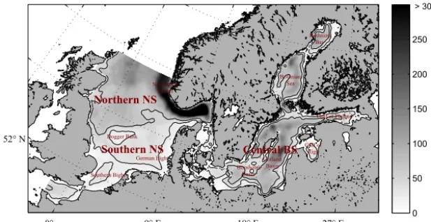
Figure 1.Model area and bathymetry. Black lines indicate the 30 and 60 m depth lines (the 60 m depth line separates the northern and southern North Sea; central BS includes all areas east of 14◦E excluding the gulf regions).
Pf Flagellates Pcyan Cyanobacteria Pd Diatoms Zl Large zooplankton Zs Small zooplankton DOM "Dissolved organic matter" D Detritus
Sed. 1 Nitrate sediment pool Sed. 2 Phosphate sediment pool Sed. 3 Silicate sediment pool
N
itr
ifi
cati
on
O2 SIO2
SiO 2•2H 2O
N2 NH4
PO4
NO3
P f Z s
Z l
P d
D
Pcyan
DOM
D
en
itr
ifi
cati
on
Sed. 3 Si Sed. 2 P Sed. 1 N
Figure 2.Schematic diagram of biological–chemical interactions in ECOSMO II (Daewel and Schrum, 2013).
and Baltic Sea on intra- and inter-annual timescales up to decadal timescales. The model was validated using nutrient observations only because of its good availability, reliability and comparability to model-estimated nutrients.
Atmospheric boundary conditions are required at the air– water interface and were taken from the NCEP/NCAR re-analysis data (Kalnay et al., 1996). Sea surface elevation, in-cluding the major tidal constituents as well as salinity and nutrients, was prescribed at the open boundaries to the North Atlantic (see Fig. 1). For the remaining ecosystem variables and temperature, a Sommerfeld radiation condition was ap-plied at the open-ocean boundaries (Orlanski, 1976). Addi-tionally, river runoffs and nutrient loads are given at the land– ocean boundary from a collection of different data sources. For more details on data sources and handling and a complete
description of the simulation set-up, please consult Daewel and Schrum (2013).
2.2 Statistical methods
cou-pled marine system, namely for the mean winter (January– March) current field and net annual primary production, and to statistically compare these modes to potential driving en-vironmental variables.
The method is comparable to the one used in Daewel et al. (2015), who gave the following brief introduction into the main elements of the analysis to clarify the terms used in the analysis.
The annual values of the spatially explicit
vari-able field form aN×Mmatrixχ (N: number of
years; M: number of wet grid points). The
em-pirical modes are given by the K eigenvectors of
the covariance matrix with non-zero eigenvalues. Those modes are temporally constant and have the
spatially variable patternpk(m=1, . . ., M) where
k=1, . . ., K. The time evolutionAk(t=1, . . ., N) of each mode can then be obtained by
project-ing pk(m) onto the original data field χ such
that χ(t, m)=
K P
k=1
pk(m)Ak(t). In the following
we will refer toAk(t) as the principal components
(PC) and to pk(m) as empirical orthogonal
func-tion (EOF). The percentage of the variance of the
fieldχ explained by modekis determined by the
respective eigenvalues and is referred to as the
global explained variance ηg(k). Before using the
method to analyse the spatiotemporal dynamics of the field, the data were demeaned (to account for the variability only) and normalized (to allow an analysis of the variability independent of its am-plitude). The identified modes are not necessarily equally significant in all grid points of the data
field. Thus, the local explained varianceηlocal,k(m)
could provide additional information about the re-gional relevance of an EOF mode and the corre-sponding PC in percent:
ηklocal(m)= "
1−Var χ(m, t)−p
k(m)Ak(t)
Var (χ(m, t))
# ·100,
(1)
where Var (X)=
N P
t=1
¯
X−X(t)2denotes the
vari-ance of the fieldX(t).
Note that in our study the data were additionally low-pass filtered using a 5-year running mean prior to applying the method. The principal modes of the EOF analysis are purely mathematical and not necessarily related to dynam-ical processes or physdynam-ically interpretable. However, the use of a proper regional and temporal window encompassing the potential scales of variability in the targeted parameter im-proves the potential for several dynamically relevant modes (Schrum et al., 2006b).
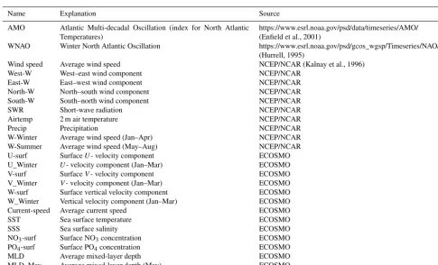
Subsequent to the EOF analysis, the major principal com-ponents (PCs) were compared through correlation analysis to equally low-pass-filtered time series of environmental vari-ables to identify potential environmental indicators and un-derlying processes. A Pearson correlation coefficient was
es-timated and tested against atdistribution to obtain a measure
for significance (Storch and Zwiers, 1999). A list of tested environmental variables is given in Table 1. These variables were averaged in time (see Table 1) and space (North Sea and Baltic Sea) prior to analysis.
2.3 Scenario simulations – design
Three types of scenarios were designed to target the specific hypothesis deduced from the statistical analysis of model re-sults and previously published hypotheses on processes be-hind ecosystem changes in the North Sea and Baltic Sea (see introduction). Here, we tested (i) the impact of short-wave ra-diation (SWR) as a parameter determining the season length and intensity of the annual primary production but which also plays a role in changes in water temperature and mixed-layer depth (MLD); (ii) the impact of the wind forcing, which af-fects not only the general current field and nutrient supply from the open ocean to the North Sea but also vertical mixing and upwelling and hence mixing of nutrients to the euphotic layer; and (iii) the ecosystem response to changes in the river nutrient loads.
Instead of just increasing or decreasing the magnitude of the forcing parameters by a certain percentage, we aimed at resolving the impacts of the multi-decadal variations in ma-jor shifts in the ecosystem dynamics. The first analysis iden-tified that the 61-year simulation period covered two differ-ent 30-year periods, for which productivity was significantly different (Daewel and Schrum, 2013). To identify the driving mechanisms for this change, we divided the 61-year simula-tion period into two climatic sub-periods (TP1: 1948–1976 and TP2: 1980–2008). Two climatic forcing variables were tested: SWR (sr) and wind stress (wi). For each of these two, scenario simulations were performed, for which all forcing variables but the target variable were kept unchanged with respect to the reference simulation. For the target variable, the forcing was repeatedly employed for both sub-periods (Fig. 3) such that in simulation 1 (sr1/wi1) the forcing from the TP1 was repeated in TP2, and in simulation 2 (sr2/wi2) the forcing from TP2 was also applied to TP1.
For the third set of scenarios we estimated average
sea-sonal cycles for the river nutrient loads (NO3, PO4, SiO) in
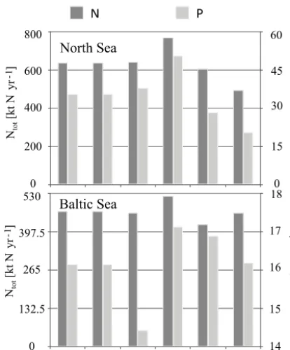
each of the six decades (Fig. 4) and performed a set of six simulations each forced by a different river load climatol-ogy. This enables us to explore the relevance of different per-sistent nutrient load situations and its relevance for abrupt changes in the system. The scenarios chosen include rela-tively high (80–89), intermediate (90–99) and low (00–08)
nutrient loads, but also unusual N/P ratios in the forcing
Table 1.Variables used for correlation analysis with principal components of the net primary production EOF analysis (Figs. 7 and 8). Both atmospheric and oceanic variables were averaged over the respective subregion (North Sea or Baltic Sea) for the analysis.
Name Explanation Source
AMO Atlantic Multi-decadal Oscillation (index for North Atlantic
Temperatures)
https://www.esrl.noaa.gov/psd/data/timeseries/AMO/ (Enfield et al., 2001)
WNAO Winter North Atlantic Oscillation https://www.esrl.noaa.gov/psd/gcos_wgsp/Timeseries/NAO/
(Hurrell, 1995)
Wind speed Average wind speed NCEP/NCAR (Kalnay et al., 1996)
West-W West–east wind component NCEP/NCAR
East-W East–west wind component NCEP/NCAR
North-W North–south wind component NCEP/NCAR
South-W South–north wind component NCEP/NCAR
SWR Short-wave radiation NCEP/NCAR
Airtemp 2 m air temperature NCEP/NCAR
Precip Precipitation NCEP/NCAR
W-Winter Average wind speed (Jan–Apr) NCEP/NCAR
W-Summer Average wind speed (May–Aug) NCEP/NCAR
U-surf SurfaceU- velocity component ECOSMO
U_Winter U- velocity component (Jan–Mar) ECOSMO
V-surf SurfaceV- velocity component ECOSMO
V_Winter V- velocity component (Jan–Mar) ECOSMO
W-surf Surface vertical velocity component ECOSMO
W_Winter Vertical velocity component (Jan–Mar) ECOSMO
Current-speed Average current speed ECOSMO
SST Sea surface temperature ECOSMO
SSS Sea surface salinity ECOSMO
NO3-surf Surface NO3concentration ECOSMO
PO4-surf Surface PO4concentration ECOSMO
MLD Average mixed-layer depth ECOSMO
MLD_May Average mixed-layer depth (May) ECOSMO
Time period 1 (TP1) 1948–1976 SWR & wind from TP1
1948 2008
Time period 2 (TP2) 1980–2008 SWR & wind from TP2
sr1:
Simulation period (years)
Short-wave radiation from TP1 Short-wave radiation from TP1
sr2: Short-wave radiation from TP2 Short-wave radiation from TP2
wi1: Wind forcing from TP1 Wind forcing from TP1
wi2: Wind forcing from TP2 Wind forcing from TP2 ref:
Figure 3. Schematic diagram for the scenario simulation set-up. The set-up is valid for the short-wave radiation experiments (sr1 and sr2) and for the wind experiments (wi1 and wi2); ref denotes the reference simulation as described in Daewel and Schrum (2013).
3 Results
3.1 Environmental indicators
To identify key long-term variations occurring in the North Sea and Baltic Sea system, we first investigated spatial av-erages of temperature, salinity and current speed for key regions. We focus here especially on the variations in the North Sea and present analysis in upper and lower water layers for the northern and southern North Sea (Figs. 5 and 6). Our analysis highlights several key characteristics related
Ntot
[
kt
N
y
r
-1]
P
O
[
kt
P
y
r
-1]
4
P
O
[
kt
P
y
r
-1]
4
Ntot
[
kt
N
y
r
-1]
Baltic Sea
530
397.5
265
132.5
0
18
17
16
15
14 60
45
30
15
0 800
600
400
200
0
North Sea
CL50-59 CL60-69 CL70-79 CL80-89 CL90-99 CL00-08
Figure 4.Decadal mean annual nutrient loadsNtot (NO3+NH4)
and PO4averaged for each of the six simulation decades for use in
the scenario simulations. Note: SiO has also been modified but is not shown here.
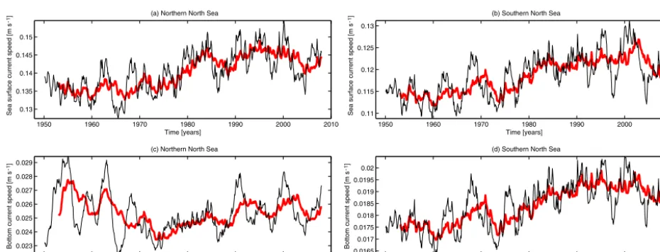
Current speed in the North Sea (Fig. 6) is dominated by a multi-decadal sinusoidal variation with low current speeds in the first 3 decades of the simulation period and higher current speeds in the later 3 decades. A contrasting trend is however found for the northern North Sea bottom layer, showing a period of minimum current speed in the intermediate simu-lation period (1970–1990). Here, a strong coupling between variability in surface and bottom layer is again identified.
The potential of statistical analysis to provide more de-tailed information on long-term variations in North Sea and Baltic Sea currents is explored through EOF analysis of cur-rent vectors. In Fig. 7 we present the mean (averaged over the 61-year time period) surface current field in the North Sea and Baltic Sea and the dominant mode from an EOF anal-ysis over the anomalies to the mean current vector field for the winter season. The analysis indicates a substantial winter inflow anomaly in the North Sea, with current speeds from northwest to southeast during the last 2 decades. Contempo-raneously, the Baltic Sea was characterized by a substantial cross-basin circulation anomaly from the Swedish coast to-wards the Polish coast that was likely related to a substantial ventilation of the Baltic Sea and nutrient transport from the lower layers to the euphotic zone as a consequence of en-hanced coastal upwelling. This nutrient enhancement in the surface would foster the Baltic Sea primary production, a de-velopment that was indeed modelled (compare Fig. 10I and explanation below). Additionally, we find substantial decadal
variability in the circulation. The first EOF thereby covers a significant part of the overall variability, with more than 60 % explained global variance. An additional EOF analy-sis performed for the scalar current speed further highlights the fact that this strong increase in strength of the northwest current component is connected to a general increase in cur-rent speed (Fig. 8c). The local explained variance in the first EOF mode (Fig. 8b) shows that this dominant mode of vari-ability (Fig. 8a) is highly relevant in the central and north-northwestern parts of the two main areas in the coupled North Sea and Baltic Sea system. However, it does not explain vari-ability in the southern and eastern coastal regions nor in the Bothnian Bay and Gulf of Finland, indicating that the current speed variability in these areas differs substantially from the dominant pattern.
3.2 Ecosystem variability
As highlighted above, changes in environmental variables are hypothesised to play a crucial role in explaining long-term changes in North Sea and Baltic Sea ecosystem dynamics. Here, we aim at identifying hydrodynamic and atmospheric indicators, which could serve as potential predictors for spa-tially resolved primary production changes. A number of in-dicators were tested, covering large-scale climate, regional atmospheric and regional hydrodynamic indicators. The pre-dictive potential of these indicators was tested and compara-tively assessed through correlations to the major PCs of pri-mary production estimates (Figs. 9 and 10).
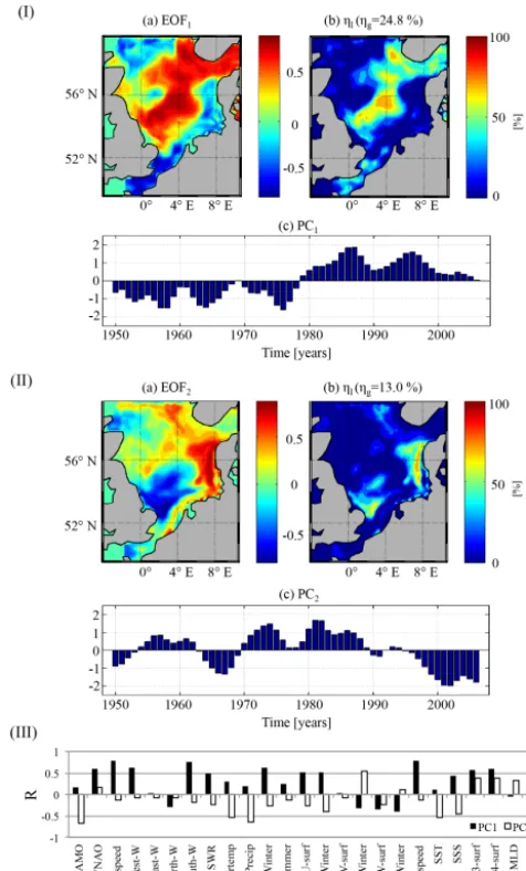
In the North Sea (Fig. 9) the first and second EOFs explain the variability in the central North Sea and in the southern frontal areas (Fig. 9I and II), featuring substantially different
temporal variability (PC1in Fig. 9Ic and PC2in Fig. 9IIc).
While in the central North Sea a major shift in primary
production was simulated around 1980 (PC1), the
produc-tion in the frontal regions passed through two major changes
(around 1970 and around 1990) (PC2). In general the signals
(PC1and PC2) were overlaid by a quasi-decadal variability,
which is comparable but not identical (partly caused by the statistical filtering procedures) to the variability estimated for the wind field.
The correlation analysis (Fig. 9III) reveals that the poten-tial indicators for production are very different for the two patterns (relevant in the different subregions). For the cen-tral North Sea, for which variability is mainly described by
the first PC (PC1, Fig. 9Ic), changes in the North Atlantic
Oscillation (NAO), changes in wind speed, specifically the western and southern wind components, and, associated with wind speed, changes in current speed show the highest cor-relations to the major mode of variability in primary produc-tion, although several other variables are also significantly
(at the 5 % level) correlated to PC1(including SWR, winter
vertical velocity, surface salinity, PO4and NO3). The
produc-tion changes in the frontal areas (PC2, Fig. 9IIc), in contrast,
1950 1960 1970 1980 1990 2000 2010 9 9.5 10 10.5 11 11.5 Time [years] (a) Northern North Sea
S S T [ oC ]
1950 1960 1970 1980 1990 2000 2010 6
6.5 7
Time [years] (b) Northern North Sea
B o tt o m t e m p e ra tu re [ oC ]
1950 1960 1970 1980 1990 2000 2010 33.7 33.8 33.9 34 34.1 34.2 34.3 Time [years] (e) Northern North Sea
Sea surface salinity
1950 1960 1970 1980 1990 2000 2010 35.05
35.1 35.15 35.2
Time [years] (f) Northern North Sea
Bottom salinity
1950 1960 1970 1980 1990 2000 2010 9.5 10 10.5 11 11.5 12 12.5 Time [years] (c) Southern North Sea
S S T [ oC ]
1950 1960 1970 1980 1990 2000 2010 9 9.5 10 10.5 11 11.5 Time [years] (d) Southern North Sea
B o tt o m t e m p e ra tu re [ oC ]
1950 1960 1970 1980 1990 2000 2010 33.6 33.7 33.8 33.9 34 34.1 34.2 34.3 Time [years] (g) Southern North Sea
Sea surface salinity
1950 1960 1970 1980 1990 2000 2010 34 34.1 34.2 34.3 34.4 Time [years] (h) Southern North Sea
Bottom salinity
Figure 5.Northern North Sea (left two columns) and southern North Sea (right two columns) temperature(a, b, c, d)and salinity(e, f, g, h) in the surface (left) and bottom layers (right). Displayed are monthly data as a 13-point moving average (black) and 61-point moving average (red).
1950 1960 1970 1980 1990 2000 2010 0.13 0.135 0.14 0.145 0.15 Time [years] (a) Northern North Sea
S e a s u rf a ce c u rr e n t sp e e d [ m s -1]
1950 1960 1970 1980 1990 2000 2010 0.023 0.024 0.025 0.026 0.027 0.028 0.029 Time [years] (c) Northern North Sea
B o tt o m c u rr e n t sp e e d [ m s -1]
1950 1960 1970 1980 1990 2000 2010 0.11 0.115 0.12 0.125 0.13 Time [years] (b) Southern North Sea
S e a s u rf a ce c u rr e n t sp e e d [ m s -1]
1950 1960 1970 1980 1990 2000 2010 0.0165 0.017 0.0175 0.018 0.0185 0.019 0.0195 0.02 Time [years] (d) Southern North Sea
B o tt o m c u rr e n t sp e e d [ m s -1]
Figure 6.Northern(a, c)and southern(b, d)North Sea surface(a, b)and bottom current speed(c, d). Displayed are monthly data as a 25-point moving average (black) and a 61-point moving average (red).
the 25 considered environmental variables. The highest cor-relations in the frontal areas can be found for the Atlantic Multi-decadal Oscillation (AMO), air temperature, and pre-cipitation. For the oceanic variables, the highest correlations can be found for SST and the stratification index early in the season (MLD_May). Despite the difference in regional and temporal variability, for both PCs the most significant indicators are linked to processes driving the surface nutri-ent concnutri-entration, which is meaningful in a system in which upper-layer primary production is limited by nutrient avail-ability. Here, the two identified regions are influenced by
dif-ferent processes. (i) Processes related to EOF1/PC1: the
long-term variability in the seasonally stratified central North Sea is mainly related to wind stress, which determines the
nutri-ent inflow from the North Atlantic to the North Sea but also impacts vertical mixing and nutrient supply to the surface
layer. (ii) Processes related to EOF2/PC2: in the frontal areas
off the Danish and English coasts and at Dogger Bank, the long-term changes in primary production are negatively cor-related to the AMO, air temperature and precipitation. The latter two variables impact the strength and timing of the sea-sonal stratification. Here the effect is inversely proportional: the warmer the temperatures, the stronger the stratification. Especially in regions with intermediate depths, a strong strat-ification and an early onset of the stratstrat-ification could substan-tially limit the nutrient supply to the euphotic zone.
− − −
Time [years]
1950 1960 1970 1980 1990 2000
4 3 2 1 0 -1 -2 -3
0.1 m s- 1 0.1 m s- 1
0.1 m s- 1 0.1 m s- 1
PC1
(a)
(b)
(c)
(e)
(d)
Figure 7.Mean surface current vectors in the North Sea(a)and Baltic Sea(b); EOF analysis of the anomalies in current vectors for the winter period January–March: current pattern for the first EOF(c, d)and first principal component(e).
first EOF mode and PC (Fig. 10I). Here, we see a clear in-crease in primary production for the time period 1950–1987 and an abrupt increase thereafter followed by an ever-so-slight decrease in primary production (Fig. 10Ic). The steep increase at the end of the 1980s has been shown to statisti-cally significantly differentiate two different periods (Daewel and Schrum, 2013) and clearly corresponds to the time
ear-lier described for a regime shift in the Baltic Sea (Alheit et al., 2005). Daewel and Schrum (2013) showed that signifi-cant changes were evident for all three phytoplankton func-tional types but that changes in cyanobacteria and flagellate production contributed most to the overall change. Hence, it
is not surprising that surface PO4 shows the highest
−
η η
− −
Time [years]
C
ur
re
nt
s
pe
ed
[
m
s
-1]
Figure 8.EOF analysis of the anomalies in current speed for the winter period January–March:(a)current speed pattern for the first EOF; (b)local explained variance;(c)first principal component.
thus processes impacting the latter must play a significant role in primary production in the Baltic Sea. Nonetheless, in contrast to the North Sea, the correlation analysis for the
Baltic Sea PC1did not indicate a dominant factor or process
that could serve as an environmental indicator for production since most of the considered parameters were found to sig-nificantly correlate to the main temporal changes in primary production (Fig. 10III). Additionally to the winter NAO, both wind speed and SWR are highly correlated to the major
pro-duction pattern (PC1). In contrast, the AMO was one of the
few parameters with no significant correlation. The second EOF (Fig. 10II) is less distinct and explains only about 6 % of variability, mostly in some coastal areas and in the Gulf
of Bothnia (Fig. 10IIb). For the related PC2(Fig. 10IIc) no
clear relationships could be identified.
3.3 Causal relationships
Since correlation analysis can identify statistical relations but not causality, we compiled subsequent scenario exper-iments with the model to identify the role of variations in wind speed, SWR and river nutrient loads for production changes in the North Sea and Baltic Sea. Those parameters were chosen due to the high correlation we found between primary production and dynamic variables related to wind field changes (wind speed, wind components, current speed) and SWR. The latter showed particularly high correlation to Baltic Sea production variability. River loads were earlier hypothesized as one of the most relevant factors responsi-ble for Baltic Sea system state changes from the late 1960s
Figure 9.(I and II)(a)First and second empirical orthogonal func-tions for annual mean primary production in the North Sea (1948–
2008); (b) local explained variance for the pattern for the
corre-sponding EOF;(c)principal component (time variation) of the
cor-responding EOF. (III) Absolute values of the correlation coefficient between the principal components (PC1 & PC2) and an environ-mental variable stated on thexaxis.
indication that the quasi-decadal variability is not attributed to wind field variations. However, in all four sub-areas the regime shifts in productivity are eroded or shifted in time when an alternative wind forcing is applied. This becomes most evident in the northern North Sea (Fig. 11b) and in the central Baltic Sea (Fig. 11c), where the long-term production variability quite closely follows the variability in the wind field and sea surface current speed (compare also Fig. 5 and correlation analysis in Figs. 8 and 9), and the major shift in experiment wi1 is displaced to the end of the 1990s follow-ing the wind forcfollow-ing dynamics from the TP1. Similar to the
Figure 10.(I and II) (a)First and second empirical orthogonal functions for annual mean primary production in the Baltic Sea
(1948–2008);(b) local explained variance for the pattern for the
corresponding EOF;(c)principal component (time variation) of the
corresponding EOF. (III) Absolute values of the correlation coeffi-cient between the principal components (PC1 & PC2) and an envi-ronmental variable stated on thexaxis.
sys-35 40 45 50 55 60 65
1950 1955 1960 1965 1970 1975 1980 1985 1990 1995 2000 2005
ref Cl50-59 Cl70-79 Cl80-89 Cl90-99
35 40 45 50 55 60
1950 1955 1960 1965 1970 1975 1980 1985 1990 1995 2000 2005
ref sr1 sr2 wi1 wi2
35 40 45 50 55 60
1950 1955 1960 1965 1970 1975 1980 1985 1990 1995 2000 2005
ref Cl50-59 Cl70-79 Cl80-89 Cl90-99
35 40 45 50 55 60
1950 1955 1960 1965 1970 1975 1980 1985 1990 1995 2000 2005
ref sr1 sr2 wi1 wi2
100 105 110 115 120
1950 1955 1960 1965 1970 1975 1980 1985 1990 1995 2000 2005
ref sr1 sr2 wi1 wi2
(a) Southern North Sea (b) Northern North Sea
(c) Central Baltic Sea (d) Gulf of Finland / Gulf of Riga
P
roduc
ti
on [
gC
m
-2 yr -1]
P
roduc
ti
on [
gC
m
-2 yr -1]
Time [years]
Time [years] Time [years] Time [years]
72 74 76 78 80 82 84 86
1950 1955 1960 1965 1970 1975 1980 1985 1990 1995 2000 2005
ref Cl50-59 Cl70-79 Cl80-89 Cl90-99
100 105 110 115 120
1950 1955 1960 1965 1970 1975 1980 1985 1990 1995 2000 2005
ref Cl50-59 Cl70-79 Cl80-89 Cl90-99
70 75 80 85 90
1950 1955 1960 1965 1970 1975 1980 1985 1990 1995 2000 2005
ref sr1 sr2 wi1 wi2
Figure 11.Estimated net primary production for the reference run (ref) and the scenario simulations concerning short-wave radiation (sr1
and sr2) and wind (wi1 and wi2)(a, b)and river nutrient load (Cl)(c, d)for two subregions in the North Sea (southern and northern North
Sea) and two subregions in the Baltic Sea (central Baltic Sea and Gulf of Finland and Gulf of Riga).
tem as seen in the two North Sea regions, where the produc-tion increase in the beginning of the 1980s is substantially enhanced by the high river nutrient loads in that decade. In-terestingly, in the central Baltic Sea this effect is not similarly apparent. Here changes in nutrient loads aggregate and result in lower or higher production, with the changes increasing slowly over time.
4 Discussion and conclusion
We identified long-term multi-decadal variations in temper-ature, salinity, currents and primary production in the North Sea and Baltic Sea from a coupled biological–physical model simulation (Daewel and Schrum, 2013). While Daewel and Schrum (2013) already identified multi-decadal changes in simulated long-term dynamics of ecosystem productivity in the North Sea and Baltic Sea, the causes and underlying pro-cesses were only speculated on in their paper. One of the ma-jor advantages of coupled ecosystem models is the availabil-ity of all information relevant for the system dynamics, in-cluding physics and forcing variables. Thus, underlying pro-cess interactions can be obtained via statistical analysis and scenario simulations.
prefer-ences for west-southwesterly wind directions”. A compara-ble mode of variability could be identified for the winter cur-rent vectors when analysed using EOF analysis. Here, both subregions (North Sea and Baltic Sea) have been analysed together, resulting in a mutual mode of variability that shows corresponding changes in winter current field anomalies after 1988 (compare Figs. 7 and 8). Mathis et al. (2015) published an EOF analysis for vertically averaged North Sea current ve-locities in winter (December–January–February) simulated over the time period 1960–2000. Although the mean current field is not directly comparable to the surface currents anal-ysed in this study, Mathis et al. (2015) concluded similarly on the relevance of the westerly wind component for the inter-annual variability in the current field and circulation pattern. Mathis et al. (2015) also found the changes in the circulation to be highly correlated to changes in the NAO. Their analysis showed that under stronger and more frequent westerly wind conditions the North Sea inflow through the Fair Isle Pas-sage was particularly enhanced, fostering a stronger south-ward flow of Atlantic water masses along the British east coast. Under opposing weather conditions, the circulation in the central and southern North Sea weakens and the inflow through the Fair Isle Passage follows the Dooley current. Thus, in that way, “effectively decoupling the water masses of the central and southern North Sea from the northern in-flow” (Mathis et al., 2015). This process proves especially relevant for the central North Sea, which is, in contrast to well-mixed areas of the southern North Sea, neither strongly exposed to water inflowing from the English Channel nor to river run-offs and can hence serve as an explanation for the provided correlation between the first mode in North Sea pri-mary production variability and the NAO and wind field.
Applying EOF analysis to primary production allows the identification of major modes of variability and their pattern together with a local indicator of explained variance. Here, the North Sea and Baltic Sea analyses led to very different results. While in the Baltic Sea we found one dominant mode that explains 67 % of the overall variability in primary pro-duction, the North Sea variability is spatially more diverse and we could identify at least two dominant modes of vari-ability linked to specific spatial hydrodynamic features of the North Sea as described in Otto et al. (1990). Although com-menting on the occurrence and relevance of actual regime shifts in the North Sea and Baltic Sea is beyond the scope of our model, the estimated primary production analysis in-deed indicated major shifts for the times when regime shifts have been identified in the literature (e.g. Dippner et al., 2012; Weijerman et al., 2005). Hence, our findings can be considered relevant for explaining major indicators for RSs in the area. Clearly the results from our study indicate that analysing long-term variability in ecosystem dynamics for an average North Sea system is not sufficient. From the regime shifts detected in the North Sea, the change in 1978–1979 ap-pears dominantly in the central North Sea (as indicated by the dominant mode of variability), while the second mode,
rele-vant in the southern North Sea frontal areas, would at least show a stronger decrease in primary production around 1990 when the second regime shift is presumed. While the sec-ond mode was correlated to air temperature and precipita-tion, environmental variables that affect the oceanic mixed-layer depths, the first mode is clearly correlated to changes in the wind and current field and resembles the variability in average sea surface currents (compare Fig. 6 and explanation of North Sea circulation). As already described above, the main processes relevant for low-frequency variations in pri-mary production of the North Sea and Baltic Sea are specifi-cally those impacting nutrient supply in the euphotic zone. Although this is in line with what has been reported for the dynamics of the 1978–1979 regime shift in Dippner et al. (2012), the variability for the central North Sea was, in contrast to their explanations, not correlated to the AMO nor to changes in the air temperature. Our results also did not support the hypothesis that changes in salinity (Lindeboom et al., 1995) or changes in sunspot activity (results not shown) (Weijerman et al., 2005) caused changes in ecosystem dy-namics. However, the identification of indicators for long-term variation assumes a priori that the indicator remains relevant for the entire time period, while studies tailored to regime shifts usually do not consider the impact on the long-term dynamics and hence might come to different results.
The Baltic Sea primary production dynamics is linked in almost the entire basin to changes in the wind field. This was particularly evident from the performed scenario runs showing that, although nutrient loads alter the magnitude of the primary production, the wind fields determine the tim-ing and magnitude of long-term variations. In Daewel and Schrum (2013), it was already pointed out that the production variability is mainly seen in the flagellates and cyanobacte-ria bloom, while the analysis presented here indicates link-age to the winter current field (compare Figs. 7 and 8). In principle the underlying process can be explained by the cause-and-effect chain proposed by Janssen et al. (2004) and the preconditioning of the deeper water column phosphate concentrations through eutrophication and anoxic conditions (Rodhe et al., 2006), which is additionally mediated by atmo-spheric conditions (Schinke and Matthäus, 1998). Thus, our results would support the hypothesis that long-term changes in primary production of the Baltic Sea are a consequence of eutrophication, even though the latter does not serve as a respective indicator for abrupt regime shifts. A similar ar-gument has been formulated in the regime shift analysis by Österblom et al. (2007).
contra-dict conclusions from Clark and Frid (2001) on the southern North Sea phytoplankton dynamics.
However, it should be pointed out that this analysis is per-formed to identify indicators for low-frequency variability; correlations are substantially weaker in unfiltered time se-ries. Moreover, climatic conditions might change and the rel-evance of specific processes for inter-annual changes in pro-duction can alter due to changes in environmental and cli-mate conditions. An example from our model study are vari-ations in North Sea nutrient loads, which caused an ampli-fication of the wind-induced variations in the 1980s in the northern North Sea as well as alterations of the primary pro-duction variability in the southern North Sea after 1990 when nutrient loads were substantially reduced. Other possible ex-amples are changes in stratification and, at least in the Baltic Sea, sea ice retreat that could cause variations in primary pro-duction and become more relevant under future climate, in which case air temperature or short-wave radiation could be-come a more significant indicator than wind speed.
Data availability. Data from the ECOSMO II long-term model in-tegration (Daewel and Schrum, 2013) and the sensitivity experi-ments are currently not publically accessible but are available on request.
Competing interests. The authors declare that they have no con-flict of interest.
Special issue statement. This article is part of the special issue “Multiple drivers for Earth system changes in the Baltic Sea re-gion”. It is a result of the 1st Baltic Earth Conference, Nida, Lithua-nia, 13–17 June 2016.
Acknowledgements. This work is a contribution to the FP7 Seas ERA SEAMAN collaborative project financed by the Norwegian Research Council (NRC-227779/E40). The authors are grateful to the two anonymous reviewers for valuable comments on an earlier version of this paper.
The article processing charges for this open-access publication were covered by a research
centre of the Helmholtz Association.
Edited by: H. E. Markus Meier Reviewed by: two anonymous referees
References
Alheit, J., Möllmann, C., Dutz, J., Kornilovs, G., Loewe, P., Mohrholz, V., and Wasmund, N.: Synchronous ecologi-cal regime shifts in the central Baltic and the North Sea in the late 1980s, ICES J. Mar. Sci., 62, 1205–1215, https://doi.org/10.1016/j.icesjms.2005.04.024, 2005.
Backhaus, J. O. and Hainbucher, D.: A Finite Difference General Circulation Model for Shelf Seas and Its Application to Low Frequency Variability on the North European Shelf, in: Three-Dimensional Models of Marine and Estuarine Dynamics, edited by: Nihoul, J. C. J. and Jamart, B. M., Elsevier Oceanography Series, 221–244, 1987.
Barthel, K., Daewel, U., Pushpadas, D., Schrum, C., Årthun, M., and Wehde, H.: Resolving frontal structures: on the payoff using a less diffusive but computationally more ex-pensive advection scheme, Ocean Dynam., 62, 1457–1470, https://doi.org/10.1007/s10236-012-0578-9, 2012.
Beare, D. J., Burns, F., Greig, A., Jones, E. G., Peach, K., Kienzle, M., McKenzie, E., and Reid, D. G.: Long-term in-creases in prevalence of North Sea fishes having southern biogeographic affinities, Mar. Ecol. Prog. Ser., 284, 269–278, https://doi.org/10.3354/meps284269, 2004.
Beaugrand, G.: The North Sea regime shift: Evidence, causes, mechanisms and consequences, Prog. Oceanogr., 60, 245–262, https://doi.org/10.1016/j.pocean.2004.02.018, 2004.
Beaugrand, G. and Ibañez, F.: Spatial, seasonal and long-term fluc-tuations of plankton in relation to hydroclimatic features in the English Channel, Celtic Sea and Bay of Biscay, Mar. Ecol. Prog. Ser., 200, 93–102, 2000.
Beaugrand, G. and Kirby, R.: Climate, plankton and cod, Glob. Change Biol., 16, 1268–1280, https://doi.org/10.1111/j.1365-2486.2009.02063.x, 2010.
Clark, R. A. and Frid, C. L. J.: Long-term changes in
the North Sea ecosystem, Environ. Rev., 9, 131–187,
https://doi.org/10.1139/er-9-3-131, 2001.
Daewel, U. and Schrum, C.: Simulating long-term dynamics of the coupled North Sea and Baltic Sea ecosystem with ECOSMO II: Model description and validation, J. Marine Syst., 119–120, 30– 49, https://doi.org/10.1016/j.jmarsys.2013.03.008, 2013. Daewel, U., Hjøllo, S. S., Huret, M., Ji, R., Maar, M., Niiranen,
S., Travers-trolet, M., Peck, M. A., Wolfshaar, and van de Wolf-shaar, K. E.: Predation control of zooplankton dynamics: a re-view of observations and models, ICES J. Mar. Sci., 71, 254–271, https://doi.org/10.1093/icesjms/fst125, 2014.
Daewel, U., Schrum, C., and Gupta, A. K.: The predictive potential of early life stage individual-based models (IBMs): an example for Atlantic cod Gadus morhua in the North Sea, Mar. Ecol. Prog. Ser., 534, 199–219, https://doi.org/10.3354/meps11367, 2015. Danielssen, D. S., Svendsen, E., and Ostrowski, M.:
Long-term hydrographic variation in the Skagerrak based on the section Torungen-Hirtshals, ICES J. Mar. Sci., 53, 917–925, https://doi.org/10.1006/jmsc.1996.0113, 1996.
Dippner, J. W., Möller, C., and Hänninen, J.: Regime shifts in North Sea and Baltic Sea: A comparison, J. Marine Syst., 105–108, 115–122, https://doi.org/10.1016/j.jmarsys.2012.07.001, 2012. Edwards, M., Beaugrand, G., Reid, P. C., Rowden, A. A., and Jones,
M. B.: Ocean climate anomalies and the ecology of the North Sea, Mar. Ecol. Prog. Ser., 239, 1–10, 2010.
Enfield, D. B., Mestas-Nuñez, A. M., and Trimble, P. J.: The At-lantic Multidecadal Oscillation and its relation to rainfall and river flows in the continental U.S., Geophys. Res. Lett., 28, 2077–2080, https://doi.org/10.1029/2000GL012745, 2001. Frank, K. T., Petrie, B., and Shackell, N. L.: The ups and downs
of trophic control in continental shelf ecosystems, Trends Ecol. Evol., 22, 236–242, https://doi.org/10.1016/j.tree.2007.03.002, 2007.
Harten, A.: High Resolution Schemes for Hyperbolic Conservation Laws, Appl. Math. Sci., 278, 260–278, 1997.
Hattam, C., Atkins, J. P., Beaumont, N., Börger, T., Böhnke-Henrichs, A., Burdon, D., Groot, R. de, Hoefnagel, E., Nunes, P. A. L. D., Piwowarczyk, J., Sastre, S., and Austen, M. C.: Marine ecosystem services: Linking in-dicators to their classification, Ecol. Indic., 49, 61–75, https://doi.org/10.1016/j.ecolind.2014.09.026, 2015.
Hurrell, J. W.: Decadal Trends in the North Atlantic Oscillation: Re-gional Temperatures and Precipitation, Science, 269, 676–679, https://doi.org/10.1126/science.269.5224.676, 1995.
Janssen, F., Schrum, C., Hübner, U., and Backhaus, J. O.: Uncer-tainty analysis of a decadal simulation with a regional ocean model for the North Sea and Baltic Sea, Clim. Res., 18, 55–62, 2001.
Janssen, F., Neumann, T., and Schmidt, M.: Inter-annual variability in cyanobacteria blooms in the Baltic Sea controlled by winter-time hydrographic conditions, Mar. Ecol. Prog. Ser., 275, 59–68, 2004.
Kalnay, E., Kanamitsu, M., Kistler, R., Collins, W., Deaven, D., Gandin, L., Iredell, M., Saha, S., White, G., Woollen, J., Zhu, Y., Leetmaa, A., Reynolds, R., Chelliah, M., Ebisuzaki, W., Higgins, W., Janowiak, J., Mo, K. C., Ropelewski, C., Wang, J., Jenne, R., and Joseph, D.: The NCEP/NCAR 40-year reanalysis project, B. Am. Meteorol. Soc., 77, 437–471, https://doi.org/10.1175/1520-0477(1996)077<0437:TNYRP>2.0.CO;2, 1996.
Lindeboom, H., Van Raaphorst, W., Beukema, J., Cadée, G. C., and Swennen, C.: (Sudden) changes in the North Sea and Wad-den Sea: oceanic influences underestimated?, Dtsch. Hydrogr. Zeitschrift, 2, 87–100, 1995.
Lynam, C. P., Llope, M., Möllmann, C., Helaouët, P.,
Bayliss-Brown, G. A., and Stenseth, N. C.:
Interac-tion between top-down and bottom-up control in marine food webs, P. Natl. Acad. Sci. USA, 114, 1952–1957, https://doi.org/10.1073/pnas.1621037114, 2017.
Mathis, M., Elizalde, A., Mikolajewicz, U., and Pohlmann, T.: Variability patterns of the general circulation and sea water temperature in the North Sea, Prog. Oceanogr., 135, 91–112, https://doi.org/10.1016/j.pocean.2015.04.009, 2015.
Möllmann, C., Kornilovs, G., and Sidrevics, L.: Long-term dynam-ics of main mesozooplankton species in the central Baltic Sea, J. Plankton Res., 22, 2015–2038, 2000.
Orlanski, I.: A simple boundary condition for unbounded
hyperbolic flows, J. Comput. Phys., 21, 251–269,
https://doi.org/10.1016/0021-9991(76)90023-1, 1976.
Österblom, H., Hansson, S., Larsson, U., Hjerne, O., Wulff, F., Elm-gren, R., and Folke, C.: Human-induced Trophic Cascades and Ecological Regime Shifts in the Baltic Sea, Ecosystems, 10, 877– 889, https://doi.org/10.1007/s10021-007-9069-0, 2007. Otto, L., Zimmerman, J. T. F., Furnes, G. K., Mork, M.,
Sae-tre, R., and Becker, G.: Review of the physical oceanog-raphy of the North Sea, Neth. J. Sea Res., 26, 161–238, https://doi.org/10.1016/0077-7579(90)90091-T, 1990.
Rodhe, J., Tett, P., and Wulff, F.: The Baltic and North Seas: A Re-gional Review of some important Physical-Chemical-Biological Interaction Processes, in: The Sea, vol. 14 B, edited by: Robin-son, A. R. and Brink, K., Harvard University Press, 1033–1075, 2006.
Schinke, H. and Matthäus, W.: On the causes of major Baltic inflows – an analysis of long time series, Cont. Shelf Res., 18, 67–97, https://doi.org/10.1016/S0278-4343(97)00071-X, 1998. Schlüter, M. H., Merico, A., Wiltshire, K. H., Greve, W., and
Von Storch, H.: A statistical analysis of climate variability and ecosystem response in the German Bight, Ocean Dynam., 58, 169–186, https://doi.org/10.1007/s10236-008-0146-5, 2008. Schrum, C.: A coupled ice-ocean model for the North Sea and the
Baltic Sea, Sensitivity of North Sea, Baltic Sea and Black Sea to anthropogenic and climatic changes, in: Sensitivity of North Sea, Baltic Sea and Black Sea to anthropogenic and climatic changes, Nato ASI Series, edited by: Özsoy, E. and Mukaelyan, A., Kluwer Academic Publishers, Dordrecht, 311–325, 1997. Schrum, C.: Regionalization of climate change for the North Sea
and Baltic Sea, Clim. Res., 18, 31–37, 2001.
Schrum, C. and Backhaus, J. O.: Sensitivity of atmosphere-ocean heat exchange and heat content in the North Sea and the Baltic Sea, Tellus A, 51, 526–549, https://doi.org/10.1034/j.1600-0870.1992.00006.x, 1999.
Schrum, C., Janssen, F., and Hübner, U.: Recent climate mod-elling in North Sea and Baltic Sea, Part A: model description and validation, Berichte aus dem Zentrum für Meeres- und Kli-maforschung Hamburg, Hamburg, Germany, 2000.
Schrum, C., Alekseeva, I., and St. John, M.: Development of a cou-pled physical–biological ecosystem model ECOSMO, J. Marine Syst., 61, 79–99, https://doi.org/10.1016/j.jmarsys.2006.01.005, 2006a.
Schrum, C., St. John, M., and Alekseeva, I.: ECOSMO, a cou-pled ecosystem model of the North Sea and Baltic Sea: Part II. Spatial-seasonal characteristics in the North Sea as revealed by EOF analysis, J. Marine Syst., 61, 100–113, https://doi.org/10.1016/j.jmarsys.2006.01.004, 2006b.
Selim, S. A., Blanchard, J. L., Bedford, J., and Webb, T. J.: Direct and indirect effects of climate and fishing on changes in coastal ecosystem services: a historical perspec-tive from the North Sea, Reg. Environ. Change, 16, 341–351, https://doi.org/10.1007/s10113-014-0635-7, 2016.
Siegismund, F. and Schrum, C.: Decadal changes in the wind forc-ing over the North Sea, Clim. Res., 18, 39–45, 2001.
Storch, H. and Zwiers, F. W.: Statistical Analysis in Climate Re-search, Cambridge University Press, The Pitt Building, Trump-ington Street, Cambridge CB2 IRP, Cambridge, UK, 1999. Thurow, F.: Estimation of the total fish biomass in the Baltic
Venegas, S. A.: Statistical Methods for Signal Detection in Climate, DCESS Report 2, Copenhagen, Denmark, 2001.
Weijerman, M., Lindeboom, H., and Zuur, A.: Regime shifts in ma-rine ecosystems of the North Sea and Wadden Sea, Mar. Ecol. Prog. Ser., 298, 21–39, https://doi.org/10.3354/meps298021, 2005.