www.earth-surf-dynam.net/4/627/2016/ doi:10.5194/esurf-4-627-2016
© Author(s) 2016. CC Attribution 3.0 License.
How does grid-resolution modulate the topographic
expression of geomorphic processes?
Stuart W. D. Grieve1, Simon M. Mudd1, David T. Milodowski1, Fiona J. Clubb1, and David J. Furbish2 1School of GeoSciences, University of Edinburgh, Drummond Street, Edinburgh, EH8 9XP, UK
2Department of Earth and Environmental Sciences, Vanderbilt University, Nashville, TN, USA
Correspondence to:Stuart W. D. Grieve ([email protected])
Received: 10 May 2016 – Published in Earth Surf. Dynam. Discuss.: 13 May 2016 Revised: 13 July 2016 – Accepted: 25 July 2016 – Published: 8 August 2016
Abstract. In many locations, our ability to study the processes which shape the Earth are greatly enhanced through the use of high-resolution digital topographic data. However, although the availability of such datasets has markedly increased in recent years, many locations of significant geomorphic interest still do not have high-resolution topographic data available. Here, we aim to constrain how well we can understand surface processes through topographic analysis performed on lower-resolution data. We generate digital elevation models from point clouds at a range of grid resolutions from 1 to 30 m, which covers the range of widely used data resolutions available globally, at three locations in the United States. Using these data, the relationship between curvature and grid resolution is explored, alongside the estimation of the hillslope sediment transport coefficient (D, in m2yr−1) for each landscape. Curvature, and consequentlyD, values are shown to be generally insensitive to grid resolution, particularly in landscapes with broad hilltops and valleys. Curvature distributions, however, become increasingly condensed around the mean, and theoretical considerations suggest caution should be used when extracting curvature from landscapes with sharp ridges. The sensitivity of curvature and topographic gradient to grid resolution are also explored through analysis of one-dimensional approximations of curvature and gradient, providing a theoretical basis for the results generated using two-dimensional topographic data. Two methods of extracting channels from topographic data are tested. A geometric method of channel extraction that finds channels by detecting threshold values of planform curvature is shown to perform well at resolutions up to 30 m in all three landscapes. The landscape parameters of hillslope length and relief are both successfully extracted at the same range of resolutions. These parameters can be used to detect landscape transience and our results suggest that such work need not be confined to high-resolution topographic data. A synthesis of the results presented in this work indicates that although high-resolution (e.g., 1 m) topographic data do yield exciting possibilities for geomorphic research, many key parameters can be understood in lower-resolution data, given careful consideration of how analyses are performed.
1 Introduction
Geomorphologists have always made use of topographic data, from initial qualitative observations of surface mor-phology and its link to process (e.g., Gilbert, 1909) to di-rectly measuring landscape geometries from contour maps, constraining river dynamics and morphometric relationships (e.g., Horton, 1932, Schumm, 1956, and Chorley, 1957). Fur-ther quantitative analyses of the Earth’s surface were fa-cilitated through the advent of gridded topographic data.
available, predominantly from light detection and ranging (li-dar), which not only refined existing techniques (Passalac-qua et al., 2010; Pelletier, 2013; Clubb et al., 2014) but also allowed the study of hitherto unresolvable features on landscapes (Tarolli and Dalla Fontana, 2009; Vianello et al., 2009; Roering et al., 2010; DiBiase et al., 2012; Tarolli, 2014; Milodowski et al., 2015b).
Presently, lidar data coverage is predominantly focused around locations of particular scientific interest or infrastruc-tural importance, as can be seen on many lidar data por-tals (e.g., Krishnan et al., 2011). It is unlikely that global li-dar coverage can be achieved in the near future, leaving the provision of commercially available 12 m TanDEM-X data (Krieger et al., 2007) and freely available 30 m Shuttle Radar Topography Mission (SRTM) data (Rabus et al., 2003) as the best available data options for many study sites.
As a consequence of this data availability it is crucial to understand the limitations of lower-resolution data when per-forming topographic analysis for geomorphic research. Ex-tracting channels from topography is a common requirement of many analyses, and it is expected that the accuracy of extracted channel networks will be affected by increasing grid resolution (Orlandini et al., 2011). Roering et al. (2007), Hurst et al. (2013b), and Grieve et al. (2016b) used mea-surements of hillslope length and relief to identify signals of landscape transience. However, all such work was performed on high-resolution topography and the impact of grid resolu-tion on these metrics is unknown. Roering et al. (2007) and Hurst et al. (2012) demonstrated that the curvature of ridge-lines measured from high-resolution topography can be used as a proxy for erosion rates in soil-mantled landscapes. This observation has been used in many studies in which cosmo-genic radionuclide-derived erosion rates are unavailable (Pel-letier et al., 2011; Hurst et al., 2013c, b; Grieve et al., 2016b). However, it can also be used in locations with an independent constraint on erosion rates in order to quantify a sediment transport coefficient that relates hillslope sediment flux to the topographic gradient, which is set by the material properties of soils (Furbish et al., 2009). Therefore, understanding the effect of grid resolution on the extraction of curvature is cru-cial in order to evaluate the applicability of calculating the sediment transport coefficient from coarse-resolution data.
Here, we grid topographic data at a range of resolutions in order to test the sensitivity of these techniques to decreas-ing grid resolution, with the aim of placdecreas-ing constraints on the estimation of common geomorphic parameters when lidar to-pographic data are unavailable. Through an analysis of one-dimensional curvature and topographic gradient approxima-tions, the changes in fidelity as grid resolution decreases for both curvature and topographic gradient are examined and placed within the context of the two-dimensional results of this study and the wider literature.
1.1 Previous work
It has long been recognized that the scale of topographic data used in an analysis or model will have an impact on the scale of the processes which can be measured (Vaze et al., 2010). It is intuitive that in order to measure the properties of hills-lope processes the resolution of the data must be high enough that variations in hillslope form can be captured adequately. The resolution of topographic data defines the Nyquist fre-quency, given as (2Res)−1where “Res” is the grid resolution of the dataset (Warren et al., 2004). The inverse of this fre-quency yields the minimum wavelength resolvable from a given dataset. In the example of a 1 m grid resolution, the smallest features that could be resolved would have a length scale of 2 m. Recognizing this, many authors have attempted to quantify this uncertainty, aiming to answer the following question: at what point does a dataset become unsuitable for a given analysis? (e.g., Quinn et al., 1991).
Many attempts to constrain the error content of topo-graphic measurements have focused on comparisons be-tween elevation values taken from differing resolution data products, often in conjunction with field survey data, with the aim of discriminating between DEM generation meth-ods. Walker and Willgoose (2006) performed a comparison of DEMs generated using cartometric and photogrammetric methods against field-surveyed elevation data. They demon-strated that at grid resolutions of 6.25, 12.5, and 25 m the car-tometric DEM produced less error than the photogrammetric DEM when compared to the field-surveyed data, collected at 3.25 m intervals.
The advent of lidar-derived topographic data provided a new technique and increased the range of possible grid reso-lutions to evaluate. Hodgson et al. (2003) assessed the qual-ity of high-resolution topographic data sourced from interfer-ometry and lidar for a heavily vegetated catchment in North Carolina. This analysis demonstrated that, under such condi-tions, the lidar-derived DEM outperformed the interferomet-ric data in addition to both classes of USGS DEM product. However, concerns were raised about the overall accuracy of the lidar data with a requirement for improved methodolo-gies to be developed to process multistory vegetation. Further work was carried out in North Carolina to constrain the min-imum number of lidar returns required to generate a DEM at a given grid resolution (Anderson et al., 2006). This work indicated that a 5 m grid (the finest resolution used) required approximately 115 points ha−1, whereas at 30 m grid reso-lution the requirement reduced to approximately 35 points ha−1.
topo-graphic maps and contour generalization, there were con-siderable errors, supporting earlier authors’ conclusions that lidar-derived topographic data contain more useful geomor-phic information than other methods of topogrageomor-phic data col-lection.
Topographic gradient (or slope) is one of the most fun-damental topographic derivatives across the disparate dis-ciplines which utilize topographic data. This measurement has been used in geomorphology (e.g., Burbank et al., 1996), ecology (e.g., Milodowski et al., 2015a), soil science (e.g., Nearing, 1997), and hydrology (e.g., Zhang and Mont-gomery, 1994). Wolock and McCabe (2000) endeavored to constrain the accuracy with which this parameter can be cal-culated as grid resolution is increased from 100 to 1000 m and showed that as the grid resolution is decreased, there is a clear reduction in the slope values produced for a landscape. Similar wide-scale analysis has also been performed within the context of global hydrological analysis (e.g., Hutchinson and Dowling, 1991, and Jenson, 1991), indicating that from meter to kilometer scale the reduction in quality of slope measurements is an issue which must be considered when working with topographic data.
Gao (1997) considered the accuracy of slope measure-ments at locations manually classified as valleys, peaks, and ridges. They found an initially small increase in the error of slope measurements at intermediate resolutions (10–20 m) and a much more rapid increase in error between 20 and 30 m resolution, suggesting a threshold minimum resolution for analysis of these landforms. More recent work has con-sidered how high-resolution lidar data impact the quality of slope measurements. Vaze et al. (2010) demonstrated a sim-ilar trend to previous authors working with lower-resolution data: as grid resolution is decreased from 1 to 25 m, there is a considerable reduction in the slope values generated for a landscape. Warren et al. (2004) evaluated the reliability of slope measurements by contrasting 10 methods of gradient calculation against field measurements of topographic gra-dient. The error between DEM and field-derived slope mea-surements was shown to increase with decreasing grid reso-lution (from 1 to 12 m), resulting in the recommendation to increase data resolution wherever possible to decrease errors in topographic analysis.
Numerous authors have considered the impact of grid res-olution on hydrological applications, which often require slope calculation as a fundamental processing step. It has been demonstrated across many landscapes and scales that as grid resolution is decreased the upslope contributing area will increase and the local slope will decrease, which will have a significant impact on any hydrological analysis (Wolock and Price, 1994; Zhang and Montgomery, 1994; Wu et al., 2008). Similarly, from the perspective of modeling global-scale sed-iment fluxes to the oceans, Larsen et al. (2014) noted that measurements of slope dropped logarithmically with increas-ing grid resolution, and failincreas-ing to account for this may lead
to a substantial underestimate of the contribution of steep, montane regions.
Kenward et al. (2000) performed analyses on the accuracy of hydrological networks generated through photogramme-try and radar interferomephotogramme-try at 5 and 30 m grid resolution, respectively. Their error analysis was extended to consider the vertical errors generated both through the downsampling of the topographic data, as well as from the techniques used to capture the topographic information. Predicted catchment runoff was up to 7 % larger in the lower-resolution datasets, considered to be driven by both the vertical errors and the reduction in spatial resolution increasing variables such as upslope drainage area.
Topographic wetness index (TWI), calculated as ln(A/S), whereAis the specific upslope area andS is the slope, is used as a single variable to compare the hydrological set-ting of differing parts of the landscape, providing insight into factors including groundwater properties and overland flow rates. Sørensen and Seibert (2007) used lidar data to test the robustness of TWI calculations on spatial scales rang-ing from 5 to 50 m, concludrang-ing that the most sensitive part of the TWI calculation was the specific upslope area mea-surements. This sensitivity resulted in significant variation in the TWI values across the range of resolutions tested. Pre-dicted slope stability, modeled in part as a function of TWI, was assessed by Tarolli and Tarboton (2006), who demon-strated that, for large-scale landsliding, a lidar-derived DEM downsampled to 10 m resolution was more suitable to iden-tify landslide hazard than the highest-resolution data avail-able. This highlights the requirement to consider the scale of the process being studied when selecting the appropriate grid resolution for a study and corresponds to the challenges of selecting the correct size of smoothing window to capture processes on a suitable scale (e.g., Roering et al., 2010, Hurst et al., 2012, and Grieve et al., 2016b).
The accuracy of channel network extraction from topo-graphic data was tested by Murphy et al. (2008), who tested a 1 m lidar DEM and a 10 m photogrammetrically generated DEM against a field-mapped channel network in a catchment in Alberta, Canada. The 1 m lidar-derived channel network was found to be the best representation of the field-mapped channel network, exceeding the quality of an additional chan-nel network mapped by hand from aerial photographs. How-ever, as no intermediate datasets were tested, it is not possible to understand at what resolution the degradation in channel network extraction quality occurs for this location.
most sensitive to resolution decreases. Work by Erskine et al. (2007) considering models of crop yields in Colorado, USA, demonstrated that on relatively flat surfaces, such as agricul-tural fields, the spatial resolution is less important than the vertical accuracy when predicting crop yields, with signifi-cant errors being produced due to centimeter-scale vertical displacements. Decreasing the grid resolution from 5 to 30 m had limited effect on the yield calculations.
Although considerable work has been carried out on the sensitivity of various factors to grid resolution, much of it has been focused on a specific application (e.g., Wolock and Price, 1994, Schoorl et al., 2000, Erskine et al., 2007, and Sørensen and Seibert, 2007) with few studies considering the impact of DEM grid resolution within a geomorphic context. Here we aim to extend existing methodologies to constrain the utility of low-resolution data products across a suite of geomorphic analyses to understand the following: (1) how hillslope length, topographic curvature, and relief vary with grid resolution; (2) how best to extract channel networks in lower-resolution datasets in order to minimize errors; and (3) whether it is possible to estimate sediment transport co-efficients from low-resolution topographic data, where an in-dependent constraint on erosion rate is available.
2 Theory and methods
2.1 Generating topographic data
Previous studies that have explored the impact of chang-ing grid resolution on topographic or geomorphic parame-ters have typically produced coarser-resolution topographic data by downsampling the highest-resolution data product available for their study sites (e.g., Thompson et al., 2001, Anderson et al., 2006, Claessens et al., 2005, and Sørensen and Seibert, 2007). Work has been undertaken to understand the influence of various re-gridding schemes on topographic measurements (Wu et al., 2008), with focus placed upon un-derstanding the use of downsampling high-resolution data in order to facilitate computationally expensive analysis on larger spatial areas with minimal loss in data fidelity. How-ever, as computational power increases, cost decreases and more efficient algorithms are developed (Tesfa et al., 2011; Qin and Zhan, 2012; Braun and Willett, 2013; Schwang-hart and Scherler, 2014), the need to downsample data for computational convenience becomes reduced. Instead, it be-comes more important to understand the limitations of avail-able data products, to facilitate geomorphic analysis in loca-tions in which high-resolution topographic data are not avail-able. This is of particular importance in many studies of nat-ural hazards (e.g., Saha et al., 2002, and Carranza and Castro, 2006) in which data quality is limited. It will also open geo-morphic research up to communities which do not have the resources to acquire high-resolution topographic data.
As a consequence of these constraints we have generated topographic data for our three study sites without
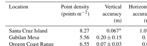
down-Table 1.Lidar point cloud metadata.
Location Point density Vertical Horizontal (points m−2) accuracy accuracy
(m) (m)
Santa Cruz Island 8.27 0.067∗ 1.07∗ Gabilan Mesa 5.56 0.20±0.15 0.11 Oregon Coast Range 6.55 0.07±0.03 0.06
∗
Accuracy is the 95 % confidence level of the root mean squared error of measurements compared to static GPS control points.
sampling or re-gridding high-resolution data products, as is commonly performed (Thompson et al., 2001; Anderson et al., 2006; Claessens et al., 2005; Sørensen and Seibert, 2007). Instead we have followed established techniques to grid the processed lidar point cloud data provided by Open-Topography (http://www.OpenOpen-Topography.org) at a range of data resolutions which span from 1 m, considered to be the limit of the Oregon Coast Range dataset by Grieve et al. (2016a) to 30 m, which is equal to the grid resolution of the global SRTM dataset (Rabus et al., 2003) and the Advanced Spaceborne Thermal Emission and Reflection Radiometer (ASTER) dataset (Yamaguchi et al., 1998) and in excess of the TanDEM-X dataset (Krieger et al., 2007) and as such should span the vast majority of grid resolutions used in mod-ern geomorphic research. The direct comparison between el-evation products generated using differing methodologies is challenging (e.g., DeWitt et al., 2015), and more work is re-quired within the context of geomorphic research to under-stand limitations in topographic datasets, such as SRTM and TanDEM-X, which arise from data capture and processing rather than purely from resolution constraints. By generating the topographic data from the same source, we aim to isolate the signal of decreasing data resolution, without the intro-duction of new sources of error which may arise from data collected using a different instrument. The error estimates of the raw point clouds used in this re-gridding process are pro-vided by OpenTopography and can be found in Table 1.
The point clouds are gridded using Points2Grid, which employs a local binning algorithm, searching for points within a circular window of radius defined by Kim et al. (2006) as
Radius= d √
2Rese. (1)
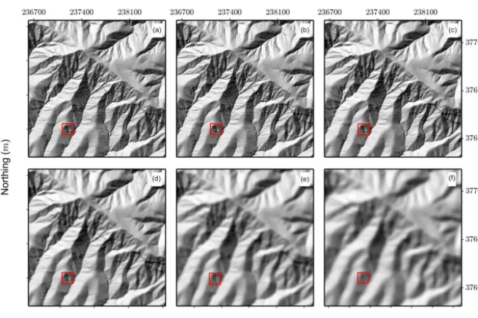
Figure 1.Example shaded reliefs of the same section of Santa Cruz Island at increasing grid resolutions. All coordinates are in UTM Zone 11◦N. Panels(a)–(f)represent resolutions of 1, 2, 5, 10, 20, and 30 m. Tick spacing is in meters. The red box outlines an extensively gullied first-order drainage, clearly visible in the highest-resolution data, but as the grid resolution is decreased, this feature and its internal structure become indistinguishable from the surrounding hillslopes.
error which must be considered when processing lidar data, and this consideration informed the selection of 1 m as the maximum resolution used in this study as it is the highest resolution these datasets can have been gridded to in the past (e.g., Perroy et al., 2010, and Grieve et al., 2016a, b).
The topographic data used in this study have been grid-ded at 20 resolutions, and Fig. 1 provides representative hill-shades of a section of Santa Cruz Island, highlighting the degradation of topographic information as grid resolution is decreased.
2.2 Measuring curvature from topography
Landscape curvature has long been recognized as a key ge-omorphic characteristic of landscapes, from Gilbert’s (1909) qualitative observations of hilltop convexity to more recent approaches to quantify landform curvature using digital to-pography (e.g., Schmidt et al., 2003, and Hurst et al., 2012). However, unlike other key landscape properties such as gra-dient (Gao, 1997; Wolock and McCabe, 2000; Warren et al., 2004; Vaze et al., 2010), hydrology (Wolock and Price, 1994; Zhang and Montgomery, 1994; Murphy et al., 2008; Wu et al., 2008), or soil characteristics (Schoorl et al., 2000; Er-skine et al., 2007), the influence of grid resolution on curva-ture has not been fully explored, particularly within a geo-morphic context.
This is particularly important with the proliferation of high-resolution topographic data from lidar, allowing the analysis of curvature on increasingly fine scales. Recent developments in channel extraction techniques (Lashermes
et al., 2007; Passalacqua et al., 2010; Pelletier, 2013; Clubb et al., 2014) typically require the identification of topo-graphic convergence in high-resolution topography using a curvature threshold. Roering (2008) and Hurst et al. (2012) demonstrated that hilltop curvature scales with erosion rate and as such demonstrated the importance of accurately con-straining the impact of grid resolution on this landscape pa-rameter. Its importance is highlighted by an increasing num-ber of studies using this relationship as a proxy for erosion rate (Pelletier et al., 2011; Hurst et al., 2013c, b; Grieve et al., 2016b). Hilltop curvature can also be used to constrain the sediment transport coefficient of a landscape where an inde-pendent constraint on erosion rate is available (Hurst et al., 2013c).
The measured curvature of a topographic surface depends on the orientation of the measurement. Here, we consider two common types of curvature, with the following definitions: (1) total curvature (CTotal) – the curvature of a surface cal-culated in two dimensions (Evans, 1980; Zevenbergen and Thorne, 1987; Moore et al., 1991) – and (2) tangential cur-vature (CTan) – the curvature calculated normal to the slope gradient (Mitášová and Hofierka, 1993). These two measures are employed to extract hilltop curvature and channel net-works, respectively. However, these definitions vary between studies and software packages; see Schmidt et al. (2003) for a full review of the varying nomenclature and definitions of curvature measurements used in the literature.
curvature from digital topographic data. It was concluded that curvature could be most accurately calculated when a nine-term polynomial was fitted to the elevation surface, with the caveat that this will only be effective where the data qual-ity is high enough. In cases in which the data are of lower accuracy, Schmidt et al. (2003) recommended using quadrat-ics to fit the elevation data. This work was extended by Hurst et al. (2012) to consider whether these patterns held for high-resolution topographic data, and it was found that fitting a six-term quadratic or nine-term polynomial yielded similar results. Therefore, Hurst et al. (2012) chose to use the six-term quadratic to compute curvature. For this study we also chose to use the six-term quadratic in order to reduce com-putation time and, more importantly, to provide more robust curvature values as the data quality is degraded to resolutions below 10 m (Schmidt et al., 2003).
We calculate curvature using a circular window passed across the landscape, with a radius defined by identifying scaling breaks in the standard deviation and interquartile range of curvature calculated at increasing window sizes, consistent with the length scales of individual hillslopes (Lashermes et al., 2007; Roering et al., 2010; Hurst et al., 2012; Grieve et al., 2016a, b). Consequently, curvature mea-surements on the hillslope scale can only be considered at data resolutions high enough to resolve individual hillslope features, considered here to be no more than 10 m, based on the window sizes identified for each landscape. A quadratic function of the form
ζ =ax2+by2+cxy+dx+ey+f (2)
is then fitted to the elevation values within the window by least squares regression (Evans, 1980), whereζ is the eleva-tion,xandyare horizontal coordinates, andathroughf are fitting coefficients. The fitted coefficients of this polynomial can be used to calculate differing types of curvature:
CTotal=2a+2b (3)
and
CTan=
2ae2−2cde+2bd2
(d2+e2)p(1+d2+e2). (4)
From the measure ofCTotal for every cell in a DEM, we can also extract a subset of curvature values from the hill-tops. The value of curvature at a hilltop (CHT) can be readily evaluated if the positions of the hilltops are known. To ex-tract hilltops we follow Hurst et al. (2012) in defining a hill-top as the boundary between two drainage basins of the same stream order. These points in the landscape can be algorith-mically extracted once a channel network is defined through the identification of points in the landscape where two chan-nels of the same Strahler order meet and the identification of that point’s upslope contributing area. Each of these ar-eas defines a basin of a given order, and by repeating this
process across the range of Strahler orders found in the land-scape, a network of hilltops can be defined. This network is then used to sample the curvature values at these locations to provide theCHTvalues across the landscape. To ensure con-sistency betweenCHT measurements at changing grid reso-lutions, the same channel network, generated using the ge-ometric method described in Sect. 2.3 from 1 m resolution data, is used as the basis of the hilltop extraction algorithm.
For our data on hilltop curvature, CHT, hilltops with a gradient exceeding 0.4 are excluded as Hurst et al. (2012) demonstrated that this gradient is the point at which> 15 % of sediment transport is nonlinear. Under nonlinear sediment flux hilltop curvature scales nonlinearly with erosion rate (Roering, 2008) and consequently cannot be used as a proxy for erosion rates. As hilltops have a convex form, their curva-ture should be negative, so as a final step any points identified as hilltops which have a positive curvature are excluded from further analysis.
2.3 Channel extraction
Extracting channel networks from digital topographic data remains a fundamental challenge for many areas of topo-graphic analysis. Without the ability to discriminate between fluvial and hillslope domains, it is not possible extract many topographic metrics such as hillslope length (Grieve et al., 2016a), mean basin slope (DiBiase et al., 2010), or hilltop curvature (Hurst et al., 2012), and the accuracy of each of these metrics will be influenced by the accuracy of the chan-nel network extracted. At a more fundamental level, the abil-ity to identify where channels initiate will facilitate better un-derstanding of the processes acting at the transition between diffusive (hillslope) and advective (fluvial) sediment trans-port (Perron et al., 2008a).
Many authors have made use of field-mapped channel heads both as a basis for geomorphic analysis and as a method for evaluating channel extraction methods (Mont-gomery and Dietrich, 1989; Orlandini et al., 2011; Julian et al., 2012; Jefferson and McGee, 2013; Clubb et al., 2014). Prior to the availability of high-resolution topographic data, contributing area and slope-area scaling thresholds were commonly used to define the location of channel heads di-rectly from DEMs (Mark, 1984; O’Callaghan and Mark, 1984; Montgomery and Dietrich, 1989; Tarboton et al., 1991; Dietrich et al., 1992, 1993). The influence of decreasing grid resolution on such channel extraction methods was evaluated by Orlandini et al. (2011), who demonstrated a strong sen-sitivity in predicted channel head location to grid resolution, suggesting that coarser-resolution data may not be suitable for channel extraction through an area threshold. We apply the method described by Orlandini et al. (2011) to quan-tify the accuracy of an extracted channel network, detailed in Sect. 2.4.
methods exploit the high-resolution nature of topographic data to resolve morphometric or process-based signatures of channel initiation or the transition between the hillslope and fluvial domain (Lashermes et al., 2007; Passalacqua et al., 2010; Pelletier, 2013; Clubb et al., 2014). Here we evaluate how two techniques – one geometric method built upon work by Pelletier (2013) and Passalacqua et al. (2010) and one process-based method, the DrEICH algorithm, developed by Clubb et al. (2014) – are influenced by decreasing grid reso-lution.
The DrEICH method was selected for evaluation as the technique on which it is based has been shown to operate suc-cessfully in lower-resolution data (Mudd et al., 2014). The DrEICH method makes use ofχ analysis, performed by in-tegrating drainage area along a river profile to facilitate com-parisons between river profiles of differing drainage area, with fewer uncertainties than traditional slope-area analysis (Royden et al., 2000; Perron and Royden, 2013). When plot-ting the χ value against elevation for a river profile, river channels will plot as linear segments, whereas hillslopes will display nonlinear segments. The DrEICH algorithm identi-fies the transition between these linear and nonlinear seg-ments as the best-fit location of the channel head.
The geometric method, used by Grieve et al. (2016b), re-moves noise from the raw topographic data using a Wiener filter (Wiener, 1949), as recommended by Pelletier (2013). This smoothed topography is then processed to identify chan-nelized portions of the landscape using a tangential curvature threshold (e.g., Pelletier, 2013), selected using the deviation of the probability density function of curvature from a nor-mal distribution on a quantile–quantile plot (e.g., Lashermes et al., 2007, and Passalacqua et al., 2010). The identified ar-eas of channelization are then combined into a contiguous channel network by employing a connected-components al-gorithm (He et al., 2008) and thinned into a final channel net-work skeleton using the algorithm of Zhang and Suen (1984). Channels were extracted from the 5, 10, 20, and 30 m DEMs generated in Sect. 2.1 using both of the channel ex-traction methodologies. Parameters required in the operation of each algorithm were selected based on values used in pre-vious studies (Grieve et al., 2016a, b), and these values can be found in Appendix A.
2.4 Comparing channel networks
To assess the accuracy of the channel networks extracted us-ing both methods, we employ two measures of quality de-scribed by Orlandini et al. (2011). These measures oper-ate on classifications of the predicted location of channel heads placing each channel head into one of three categories: true positives (TPs), false positives (FPs), and false nega-tives (FNs). A TP is where a predicted channel head from low-resolution data occupies the same spatial location as the channel head derived from 1 m resolution topography. An FP is where a predicted channel head is placed in a
loca-tion where there is no channel head in the high-resoluloca-tion data. An FN is when a channel head from high-resolution to-pography does not have a predicted channel head from low-resolution topography in the same spatial location.
We follow Orlandini et al. (2011) in employing a 30 m search radius around the 1 m derived channel heads and con-sider a low-resolution channel head falling within this radius to be spatially coincident. This has the effect of normalizing the size of each channel head point, to ensure that we can perform comparisons between predictions made at different spatial resolutions.
The reliability, r, of a channel extraction method is the ability of a method to not predict channel heads in areas where none are located and is calculated as
r= P
TP P
TP+FP, (5)
whereP
TP is the total number of true positives andP FP is the total number of false positives. The sensitivity,s, of a channel extraction methodology is given by
s= P
TP P
TP+P
FN, (6)
where PFN is the total number of false negatives. The sensitivity is the ability of a method to predict all of the channel heads expected. Using these two indexes it is pos-sible to quantify the quality of channel heads predicted using low-resolution data, as well as understand why a particular method fails, by distinguishing between methods which fail due to either over- or underpredicting the number of channel heads in a landscape or by simply placing channel heads in the wrong spatial location.
2.5 Estimating the hillslope sediment transport coefficient from hilltop curvature
The sediment transport coefficient,D[L2T−1] (dimensions of mass [M], length [L], and time [T] denoted in square brackets), of a landscape is a measure of its sediment trans-port efficiency and was demonstrated by Furbish et al. (2009) to be controlled by the material properties of soil such as grain size, cohesion, and thickness. The value ofD within a landscape will exert a control on the morphology of hill-slopes (e.g., Roering et al., 1999). Diffusion-like hillslope evolution can be modeled using a 1-D mass conservation equation, assuming that the contribution to surface lowering from chemical processes is negligible when contrasted with the signal of surface lowering from physical processes (e.g., Roering et al., 1999, and Mudd and Furbish, 2004):
ρs ∂ζ ∂t = −ρs
∂qs
∂x +ρrU, (7)
U[L T−1]is the uplift rate. In steady-state landscapes, where U=Eand∂ζ /∂t=0, Eq. (7) simplifies to
ρr ρs
E=∂qs
∂x, (8)
withE[L T−1]denoting the erosion rate. To solve this equa-tion, a statement of the volumetric sediment flux per unit con-tour length,qs[L2T−1], must be derived. A nonlinear rela-tionship between sediment flux and topographic gradient has been proposed by a number of authors (Andrews and Buck-nam, 1987; Koons, 1989; Anderson, 1994; Howard, 1997; Roering et al., 1999, 2001; Pelletier and Cline, 2007). Sup-port for such models has been found from both tests of the resulting topographic predictions (Roering et al., 2007; Hurst et al., 2012; Grieve et al., 2016a) as well as through indepen-dent measurements of sediment flux across hillslopes (Roer-ing et al., 2001; Roer(Roer-ing, 2008).
The nonlinear model proposed by Andrews and Bucknam (1987) and Roering et al. (1999) is of the form
qs=DS "
1− |S|
Sc 2#−1
, (9)
whereScis a critical gradient, and as the hillslope gradient approaches this threshold,qsasymptotes towards infinity.
At low hillslope gradients (e.g., on hilltops), the term within brackets in Eq. (9) approximates to unity (Hurst et al., 2012). Equation (9) can therefore be substituted into Eq. (8) and can be solved forD on low-gradient hilltops, assuming that an independent constraint onEis available,
D= − Eρr CHTρs
. (10)
2.6 Hillslope length and relief
Hillslope length (LH) is a crucial landscape parameter to constrain as it controls the rate of mass flux by overland flow within catchments (Dunne et al., 1991, 2016; Thomp-son et al., 2010), influences rates of soil erosion (Liu et al., 2000), and presents a first-order control on the maximum source area of landslides (Hurst et al., 2013a). Furthermore, it may be used to demonstrate nonlinearity in hillslope sed-iment flux (Roering et al., 1999, 2007; Grieve et al., 2016a, b).
Many studies have attempted to calculate hillslope length through the inversion of drainage density (Tucker et al., 2001), analysis of plots of local slope against drainage area (Roering et al., 2007), direct measurements from topographic maps (Hovius, 1996; Talling et al., 1997), and by mea-suring the length of overland flow from ridgeline to chan-nel (Hurst et al., 2012; Grieve et al., 2016a). Grieve et al. (2016a) demonstrated that the most geomorphologically suit-able technique to use, particularly in the context of hillslope
sediment transport, was that of measuring the length of over-land flow. An additional measure which can be derived from this technique is the topographic relief, which is the differ-ence in elevation between a hilltop and channel connected by a hillslope flow path. Topographic relief has been esti-mated in a number of ways and is frequently used in studies of tectonic geomorphology (e.g., Gabet et al., 2004, Hilley and Arrowsmith, 2008, Gallen et al., 2011, and Gallen et al., 2013). Furthermore, topographic relief may be used to gen-erate dimensionless erosion and relief plots (Roering et al., 2007; Hurst et al., 2012; Sweeney et al., 2015; Grieve et al., 2016b), which can be used to identify landscape transience (Hurst et al., 2013b; Mudd, 2016). Consequently, we intend to test the robustness of measuring hillslope length and re-lief as grid resolution decreases, with the aim of facilitating increased confidence in geomorphic analyses performed in locations where high-resolution topography is unavailable.
Using the 20 topographic datasets generated in Sect. 2.1 for each of the three landscapes, hillslope length measure-ments were generated following the methods outlined in Grieve et al. (2016a). We measured hillslope length on each dataset using two different channel networks. Firstly, chan-nel heads were extracted from the highest-resolution data set, in each case 1 m, using the geometric method outlined in Sect. 2.3. These high-resolution channel heads were mapped onto the coarser-resolution topographic data, to ensure that changing channel extraction results will not have an influ-ence on the measures of hillslope length. This allows im-proved isolation of the factors driving variations in hillslope length as grid resolution is decreased. Secondly, the analy-sis was performed using coarser-resolution channel networks extracted using the geometric method of channel extrac-tion. We use the geometric method as opposed to the DrE-ICH method because, as we will show below, the geometric method is less sensitive to grid resolution. These two channel networks effectively provide upper and lower bounds for the accuracy of hillslope length and relief measurements.
3 Study sites
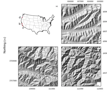
Figure 2.(a)Map showing the location of each of the study sites within the USA.(b–d)Shaded reliefs of representative sections of each study site, generated from 1 m resolution data. Tick spacing is in meters. All coordinates are in UTM.(b)Gabilan Mesa, California, UTM Zone 10◦N.(c)Santa Cruz Island, California, UTM Zone 11◦N.(d)Oregon Coast Range, Oregon, UTM Zone 10◦N.
a more challenging test case for our analyses. Furthermore, these sites were selected as they each have high-resolution li-dar data covering a large spatial area and have been the sub-ject of many previous studies (Reneau and Dietrich, 1991; Roering et al., 1999, 2001; Montgomery, 2001; Pinter and Vestal, 2005; Roering et al., 2007; Perron et al., 2009; Per-roy et al., 2010, 2012; Marshall and Roering, 2014; Grieve et al., 2016a, b), which should provide a good basis for the evaluation of the results of this study in a wider geomorphic context.
3.1 Gabilan Mesa
Gabilan Mesa, a section of the Central Coast Ranges in Cali-fornia, USA (Fig. 2b), is a highly regular landscape with very gentle transitions between hillslopes and channels, which correspond to topographic predictions of diffusion-like sed-iment transport (Roering et al., 2007). The area’s semiarid climate supports a range of vegetation from oak savanna to chaparral shrubland (Shreve, 1927; Roering et al., 2007). The nature of this lower-density vegetation allows a larger portion of lidar pulses to reach the ground, requiring less pro-cessing and interpolation to generate a final bare-earth DEM for analysis (Liu, 2008; Meng et al., 2010).
A series of large, linear canyons running northeast to southwest are fed by parallel tributaries which flow perpen-dicular to the main trunk channel. These regularly spaced valleys present two distinct length scales in the landscape which have been observed both qualitatively (Dohrenwend, 1978, 1979) and quantitatively through measurements of hill-slope length distributions (Grieve et al., 2016a). Relation-ships between dimensionless erosion rate and relief, the uni-formity of hilltop curvatures, and the regularity of valley spacing have all been used to assert that much of this land-scape is in steady state (Roering et al., 2007; Perron et al., 2009; Grieve et al., 2016b), although localized observations of a relict plateau surface add complexity to this steady-state observation.
3.2 Santa Cruz Island
Figure 3.Maps showing the spatial variation in total curvature measurements as grid resolution is decreased for the same section of Santa Cruz Island as displayed in Fig. 1. All coordinates are in UTM Zone 11◦N. Panels(a)–(f)represent resolutions of 1, 2, 5, 10, 20, and 30 m. Tick spacing is in meters. The black boxes outline the same features as highlighted in Fig. 1, showing the reduction in the curvature signal with grid resolution for such a feature.
and Vestal, 2005); this regular pattern is particularly evident in the northwest section of the study area. The Santa Cruz Fault has been demonstrated to have left-lateral strike slip motion, which deflects channels away from the perpendicular to the main valley in the center of the island (Pinter et al., 1998). Studies of marine terraces in the region suggest that the Channel Islands have been steadily uplifted through the late Quaternary (Muhs et al., 2014).
The island has a Mediterranean climate similar to that of Gabilan Mesa (Pinter and Vestal, 2005), supporting exten-sive grassland with occasional patches of pine forest and cha-parral vegetation (Pinter and Vestal, 2005; Perroy et al., 2010, 2012). Human activities led to overgrazing across the island at the turn of the 19th century, causing a period of gullying and rapid erosion, particularly evident in the southwest of the island (Pinter and Vestal, 2005; Perroy et al., 2012). The lidar data collected for this location have been extensively tested and ground truthed, ensuring that they are suitable for use in a geomorphic context (Perroy et al., 2010) and for perform-ing topographic analysis at high spatial resolutions.
3.3 Oregon Coast Range
The Oregon Coast Range in Oregon (Fig. 2d), USA, is a densely vegetated upland landscape, dominated by conifer-ous and hardwood forests (Schmidt et al., 2001), with a hu-mid climate (Roering et al., 1999). Qualitative observations of the landscape suggest that the valleys are regularly spaced, with a particular uniformity found in the dimensions of
first-order drainage basins (Roering et al., 1999, 2007; Marshall and Roering, 2014). Such observations have been supported by measurements of hillslope length across the landscape (Grieve et al., 2016a). However, comparisons of the dimen-sionless relief and erosion rate performed by Grieve et al. (2016b) highlight the small-scale topographic variability in-herent in this otherwise regular landscape. The Oregon Coast Range is considered to be in steady state due to the corre-lation between uplift rates from marine terrace data (Kelsey et al., 1996) and erosion rates from cosmogenic radionuclides (Beschta, 1978; Reneau and Dietrich, 1991; Bierman et al., 2001; Heimsath et al., 2001). The hillslopes are steeper and the ridgelines sharper than in Gabilan Mesa, consistent with observations of debris flows and shallow landsliding across the range (Dietrich and Dunne, 1978; Heimsath et al., 2001; Montgomery, 2001), which have the potential to create a dis-tinct topographic signature (Booth et al., 2009).
4 Results
4.1 Curvature
Figure 4.Plots of the distribution ofCTotal (a, c, e) andCTan (b, d, f)measurements as resolution is decreased for each of the study
landscapes. Whiskers are the 2nd and 98th percentiles; the box covers the 25th and 75th percentiles; the blue bar is the mean and the red bar is the median. The gray outline is the probability density function of each dataset.
signal of this first-order feature being lost as the grid resolu-tion approaches 30 m.
Figure 4 displays the variations in the distribution of total and tangential curvature measurements with grid resolution for each of the study landscapes. Santa Cruz Island shows lit-tle variation in mean and median curvature with resolution, with the majority of the changes in each distribution with res-olution occurring at the extremes of the curvature distribution for each dataset, as the representation of ridgelines and chan-nel bottoms becomes increasingly diffuse. As resolution is decreased, the range between 2nd and 98th percentiles and the 1st and 3rd quartiles decreases, with a more rapid reduc-tion in the more extreme values than in the quartiles (Fig. 5). While this effect is most marked at the extremes, the distribu-tions are condensed across all percentile intervals as grid
res-olution is increased beyond 3–4 m. This behavior is observed for bothCTotalandCTanas grid resolution is decreased.
Figure 5.Plots of the reduction in range between the 2nd and 98th percentiles (blue triangles) and the interquartile range (red circles) of CTotal(a, c, e)andCTan(b, d, f)measurements as resolution is decreased for each of the study landscapes.
4.2 Channel networks
Figure 6 provides a qualitative overview of the changes of channel network extent with decreasing grid resolution for both methods, across the three test landscapes. In each case the general patterns are that as the grid resolution is de-creased, the lowest-order channels are lost, as they exist on a spatial scale below that of the data resolution. In contrast, large parts of the predicted networks appear to occupy sim-ilar spatial locations in larger, higher-order channels where the topographic signal of a channel is more pronounced. The geometric method shows less reduction in drainage density than the DrEICH method, as data resolution is decreased.
Figure 7 provides a quantitative assessment of channel ex-traction quality by presenting the indexes of reliability and sensitivity for both the geometric channel extraction and
Figure 6.Representative sections of each landscape’s channel network displaying the extent of each network as grid resolution is decreased. Panels (a), (b), and(c) are generated using the DrEICH method of channel extraction. Panels(d), (e), and (f)are generated using the geometric method. All coordinates are in UTM. Tick spacing is in meters. The left column is from Santa Cruz Island, UTM Zone 11◦N, the central column is from Gabilan Mesa, UTM Zone 10◦N, and the right column is from the Oregon Coast Range, UTM Zone 10◦N.
Figure 7.The variations in reliability (Eq. 5) and sensitivity (Eq. 6) of each channel network with decreasing grid resolution. Panels(a), (c), and(e)are generated using the geometric method of channel extraction. Panels(b),(d), and(f)are generated using the DrEICH method. The top row is from Gabilan Mesa, the middle row is from Santa Cruz Island, and the bottom row is from the Oregon Coast Range. The full results from this analysis can be found in Tables 3 and 4.
In Santa Cruz Island the geometric method’s reliability in-dex is similar to Gabilan Mesa; however, the sensitivity inin-dex is not as high, which indicates that a large number of channel heads are being missed, but where a prediction is made, it is typically accurate. The DrEICH method exhibits a similarly large reliability initially but again shows more rapid
degra-Figure 8.Changes in the estimated sediment transport coefficient, D, calculated using Eq. (10) and parameters in Table 2 for each of the three study landscapes, with decreasing data resolution. The error bars on each data point represent the uncertainties reported for each landscape’s erosion rate data.
dation in the index value as grid resolution is decreased. The sensitivity values again decline more rapidly and reach a 0 value at 20 m grid resolution.
re-Table 2.Published parameters used to calculate diffusivity.
Location Soil density Rock density Erosion rate Reference (kg m−3)∗ (kg m−3)∗ (mm yr−1)
Santa Cruz Island 1.4 2.4 0.069±0.007 Perroy et al. (2012) Gabilan Mesa 1.4 2.4 0.36+−00..3822 Roering et al. (2007) Oregon Coast Range 1.4 2.4 0.1±0.05 Roering et al. (1999)
∗Soil and rock densities are representative of typical measurements of the field sites and are taken from Hillel (1980).
Table 3.Reliability and sensitivity metrics for the DrEICH method of channel extraction.
Location Resolution (m) P
TP P
FP P
FN r s
Gabilan Mesa 5 555 982 1489 0.36 0.27
10 210 879 1875 0.19 0.1
20 42 734 2088 0.05 0.02
30 13 609 2122 0.02 0.01
Santa Cruz Island 5 3295 1971 4799 0.63 0.41
10 2454 793 6865 0.76 0.26
20 69 838 8235 0.08 0.01
30 27 915 8284 0.03 0.0
Oregon Coast Range 5 507 1718 1131 0.23 0.31
10 144 445 1462 0.24 0.09
20 16 105 1623 0.13 0.01
30 2 442 1639 0.0 0.0
Table 4.Reliability and sensitivity metrics for the geometric method of channel extraction.
Location Resolution (m) P
TP P
FP P
FN r s
Gabilan Mesa 5 1019 519 987 0.66 0.51
10 712 380 1301 0.65 0.35 20 448 332 1592 0.57 0.22 30 292 333 1775 0.48 0.14
Santa Cruz Island 5 4280 991 3109 0.81 0.57
10 2473 777 4998 0.76 0.33
20 334 505 7861 0.4 0.04
30 475 470 7659 0.5 0.06
Oregon Coast Range 5 792 1438 788 0.36 0.5
10 562 602 938 0.48 0.37
20 276 374 1275 0.42 0.18 30 475 277 1418 0.38 0.11
liability indexes and steadily decline towards 0. A sensitiv-ity value exceeding the reliabilsensitiv-ity value suggests that in this landscape there are fewer missed channel heads in the 5 m data but at the expense of too many predicted channel heads in locations where there are none predicted in the 1 m data.
4.3 Sediment transport coefficient
Using the values for hilltop curvature generated in Sect. 4.1, published parameters for erosion rate and material properties
Figure 9.Plots of the distribution of hillslope length(a, c)and relief(b, d)measurements as resolution is decreased for Santa Cruz Island. Whiskers are the 2nd and 98th percentiles; the box covers the 25th and 75th percentiles; the blue bar is the mean and the red bar is the median. The gray outline is the probability density function of each dataset. The top row presents the best-case scenario, where an independent constraint on the channel network is available for the lower-resolution data, and the bottom row uses the channel networks extracted using the geometric method outlined in Sect. 2.3 for each resolution step.
Range and Santa Cruz Island datasets exhibit an increase in estimatedD, all of the values for each location fall within the range of values forDcompiled by Hurst et al. (2013c).
4.4 Hillslope length and relief
The hillslope length measurements for Santa Cruz Island cal-culated using 1 m channel heads (Fig. 9a) show little varia-tion in the distribuvaria-tion of the data up to 10 m resoluvaria-tion, with the main difference being the decrease with grid resolution in the 2nd percentile measurements, which is a trend observed within each of the datasets. The mean and median values also gradually decrease towards the 10 m resolution dataset, be-fore gradually increasing towards the 30 m resolution step. However, these variations are very small, with the overall distributions of hillslope length and relief not varying con-siderably between resolution steps. When the same hillslope length algorithm is applied using channel networks extracted using the geometric method for each resolution step (Fig. 9c), there is little change in the distribution or average values of LHuntil beyond the 10 m resolution step. Beyond this point the measurements of hillslope length are clearly affected by the reduction in accuracy of the channel network. The relief measurements for both channel head methods (Fig. 9b, d) in Santa Cruz Island exhibit little resolution dependence up to 10 m grid resolution, beyond which point the values increase steadily. In the case of the 1 m channel heads, the distribution becomes compressed around the average values at lower res-olutions, whereas with the variable channel head dataset the distribution of values increases with decreasing resolution.
In Gabilan Mesa the hillslope length measurements cal-culated using 1 m channel heads (Fig. 10a) show a gradual reduction in mean and median values between the highest-resolution data and the 8 m highest-resolution data before a small plateau and then a small increase until the 30 m dataset. The average relief values calculated for the same dataset increase steadily by approximately 20 m between the highest- and lowest-resolution datasets (Fig. 10b). The distribution of re-lief measurements are broadly consistent between 1 and 5 m resolutions before reducing about the median as grid resolu-tion is decreased. The same trends are apparent in the hills-lope length and relief data calculated using the variable chan-nel heads (Fig. 10c, d) with little change between the two pairs of datasets.
Figure 10.Plots of the distribution of hillslope length(a, c)and relief(b, d)measurements as resolution is decreased for Gabilan Mesa. Whiskers are the 2nd and 98th percentiles; the box covers the 25th and 75th percentiles; the blue bar is the mean and the red bar is the median. The gray outline is the probability density function of each dataset. The top row presents the best-case scenario, where an independent constraint on the channel network is available for the lower-resolution data, and the bottom row uses the channel networks extracted using the geometric method outlined in Sect. 2.3 for each resolution step.
range of resolutions from 1 to 10 m, where the fixed data show much less variation.
5 Discussion
5.1 Curvature and the problem of resolution-dependent filtering
Across the three landscapes the variance of the distributions of both total and tangential curvature values are systemat-ically reduced as resolution is decreased, an effect that is particularly notable after the grid resolution exceeds 3–4 m (Fig. 4). In each of the three datasets, the interquartile ranges remain relatively constant, whereas beyond 4 m resolution in each case the range between the 2nd and 98th percentiles re-duces rapidly (Fig. 5), demonstrating that the majority of the loss of curvature information occurs at the extremes of the distribution.
In producing a DEM, we are sampling a complex two-dimensional elevation signal, in which spatial variations in geomorphic processes drive variations in topographic am-plitude at different wavelengths (Perron et al., 2008b). De-creasing the grid resolution of DEMs acts as a low-pass filter on this topographic signal, which preferentially de-grades features in the topography that have significant am-plitude at small wavelengths, such as sharp ridgelines, nar-row valley bottoms, and local topographic roughness gener-ated by, for example, landslides, tree throw, and rock expo-sure (Figs. 1 and 3). While the position of ridges and val-leys is preserved in coarser-resolution data, the magnitude of their associated curvature values is reduced as resolution decreases; this effect is particularly marked for hillslopes in which curvature is focused at the ridge crest and valley bottoms, a common characteristic of more rapidly eroding landscapes (Roering et al., 1999, 2007). For first-order land-scape features, such as gullies, landslide scars, and first-order channels, decreasing grid resolution eventually results in the complete loss of topographic information, as highlighted in Figs. 1 and 3.
5.1.1 Topographic filtering and its implications for curvature and slope measurements
We can explain some of the observed behavior in Figs. 4 and 5 through spectral analysis. Spectral analysis assumes that data can be approximated as the sum of sine waves of varying frequency. One can apply a spectral filter to any dataset: this simply means that one transforms input data into output data using linear functions (that is, we can multiply the input data by a series of weights). Any filter will have again, which is the ratio between the filtered amplitude and the original amplitude. A filter will also have afidelity, which is the ratio between the continuous gain and the discrete gain. We are using discrete data, so the fidelity measures how well our discrete filter is able to reproduce a theoretical signal that
is continuous. We can never have continuous data since lidar is not continuous: our filters will always represent an fect version of nature and fidelity quantifies just how imper-fect it is. Hopefully our readers will not be put off by this foray into jargon, and we can move on to practical applica-tion of spectral filters for use in topographic applicaapplica-tions.
We will examine the spectral behavior of a simplified one-dimensional system. We acknowledge that a 1-D approach cannot fully describe complex two-dimensional topography of real landscapes, but a one-dimensional system is amenable to mathematical treatment that can at least give us qualitative insight into trends observed in our data. In addition, some of the features of interest, for example ridgelines and channels, can be roughly approximated as one-dimensional structures within a two-dimensional landscape.
Curvature in one dimension,Cx [L−1], is often
approxi-mated with the differencing equation:
Cx=
ζ(x−1x)−2ζx+ζ(x+1x)
(1x)2 , (11)
whereζ [L] is the elevation of the land surface,x [L] is a location in space,Cx is the curvature at locationx, and1x
[L] is the grid interval. The subscripts denote the discrete lo-cations where elevation is evaluated. Equation (11) is in fact a spectral filter. The original data isζ, which is distributed in space, and the weights in the filter are (1x)−2,−2(1x)−2, and (1x)−2for data points at (x−1x),x, and (x+1x), re-spectively. From this filter, we can calculate thewave number response function. A full description of the theory and signif-icance of a wave number response function can be found in Jenkins and Watts (1968). For our purposes, it is sufficient to know that this function must be calculated if we are to calculate the gain and fidelity of the filter (which here is a measure of curvature of our elevation data). The wave num-ber response function (H(ω;1x)) from this filter, given by Jenkins and Watts (1968) in their Eq. (7.3.7), is
H(ω;1x)= 2
(1x)2[cos(ω1x)−1], (12)
where ω=2π/L[L−1] is the wave number with wave-length L [L]. Higher wave numbers correspond to shorter wavelengths. Using this function, we can calculate the gain, G(ω;1x). Again, the gain measures the ratio of the tude of the filtered signal (in this case curvature) to the ampli-tude of the original signal (in this case elevation) at the wave numberω. The theoretical gain for continuous waveforms of curvature (i.e., not discrete filters like Eq. 11) isω2. The gain of a discrete filter is the modulus of the wave number response function (see p. 296 in Jenkins and Watts, 1968), so in the case of Eq. (12) the resultant gain,G(ω;1x) is
G(ω;1x)= 2
(1x)2[1−2 cos(ω1x)+cos
2(ω1x)]1/2. (13)
Figure 12.Plot of fidelity (F) of two one-dimensional differencing operations: curvature (Eq. 11) and topographic gradient (Eq. 15) as a function dimensionless wave number1x/Lto the Nyquist wave number,1x/L=0.5.
crests, tree throw mounds, local roughness) in the elevation data involve relatively large values of curvature, whereas low-frequency elevation waveforms (e.g., ridge–valley fea-tures or geologic folds) with the same amplitude involve rela-tively small curvatures. Crucially, however, the discrete filter does not retain all of the high-frequency information. Some of this information is lost in the discretization process (i.e., it is lost because we are sampling the data at fixed intervals rather than having continuous information about the surface). We can calculate what information is lost by calculating the fidelity, which is the ratio between discrete gain (Eq. 13) and the theoretical gain (ω2):
F(ω;1x)= (14)
2
(1x)2ω2[1−2 cos(ω1x)+cos
2(ω1x)]1/2.
Again, fidelity is a measure of how closely our discrete filter (here curvature measured at discrete points in the land-scape) reflects the true curvature (that is, the curvature mea-sured if we had a perfectly continuous dataset). Fidelity is a function of the ratio between the grid interval and the wave-length (Fig. 12). When the fidelity is unity, the discrete fil-ter exactly reproduces the underlying continuous function. Again, the landscape (and its derivative metrics like curva-ture and gradient) has feacurva-tures at different wavelengths, such as long-wavelength ridges and valleys and short-wavelength tree throw mounds.
As the frequency approaches the Nyquist wave number, defined as 1x/L=1/2, fidelity decreases (Fig. 12); a fi-delity of only approximately 0.4 is achieved at the Nyquist wave number itself. To achieve a fidelity,F, of 0.9 requires
that L/1x is equal to approximately six grid points per wavelength. A fidelity F=0.95 requires eight points per wavelength, andF =0.99 requires 18. Therefore, while the grid resolution imposes a minimum wavelength that can be resolved (defined by the Nyquist wave number), the behavior of the fidelity function (Fig. 12), clearly illustrates that cur-vature information will be lost when calculated for features with wavelengths greater than but still close to the minimum resolvable at the Nyquist wave number.
What does this mean in practical terms? In our simple, one-dimensional example, if we use 1 m resolution data we can only capture the curvature of a one-dimensional ridgeline that had a wavelength of 3–4 m (one does not need the entire wave to capture the peak of the waveform) but with a loss of fidelity on the magnitude of the curvature. Or, in other words, we would underestimate the magnitude of the curvature.
Another landscape metric that is widely measured is topo-graphic gradient. In our study we have not computed how to-pographic gradient varies as a function of grid resolution be-cause this has been examined by many previous authors (e.g., Gao, 1997, Warren et al., 2004, and Vaze et al., 2010). How-ever, our treatment of the properties of a one-dimensional filter can give some insight into previous results. Consider a simple central-difference approximation of the topographic gradient (Sx, dimensionless):
Sx=
ζ(x+1x)−ζ(x−1x)
21x . (15)
Equation (15) is yet another spectral filter, with weights of 2(1x)−1atx+1xand−2(1x)−1atx−1x. We can follow the same series of operations that we performed on Eq. (11) to arrive at the fidelity of Eq. (15), denoted asFS, taking into account that the theoretical gain isω(see Eq. 7.3.8 in Jenkins and Watts, 1968):
FS(ω;1x)= 1
1xω[sin(ω1x)]. (16)
5.1.2 Total and tangential curvature
Having explored simplified one-dimensional filters, we now return to our two-dimensional results. Although real land-scapes are two-dimensional and we use polynomial fitting rather than simple differencing as in Eq. (11), we can still use Eq. (14) as a qualitative indicator of the grid resolution required for appropriate curvature estimates. In the Gabilan Mesa, where ridgelines are broad, lower-resolution data can still capture the curvature with relatively high fidelity. How-ever, in locations with sharper ridgelines, such as Santa Cruz Island, the narrowest ridgelines are no longer adequately re-solved as the grid resolution is decreased, as can be seen in Fig. 3.
The loss of fidelity predicted by the simple one-dimensional system (Eq. 14) qualitatively predicts the pat-tern observed in Figs. 4 and 5, namely that the curvature val-ues are smeared over a greater length scale leading to ap-parently broader ridges with resolution and a systematic un-derestimation of their peak elevations. This highlights that in conjunction with data quality, landscape morphology also exerts a control on the optimal resolution to use for a given study, where landscapes with more gradual hillslope to val-ley transition morphologies can be analyzed using coarser-resolution topographic data with more confidence. Although the identification of landscape morphology is often achieved through observations of high-resolution topography, it can be achieved through field observations and the use of ancillary datasets, which allow the qualitative checking of results ob-tained from a low-resolution dataset.
Santa Cruz Island and the Oregon Coast Range have the highest tangential curvature at 1 m resolution. High tangen-tial curvature at Santa Cruz Island corresponds to observa-tions of extensive gullying and hillslope erosion (Pinter and Vestal, 2005; Perroy et al., 2012). In the Oregon Coast Range, features such as pit and mound topography produced by tree throw and other biotic activity are resolved in the lidar dataset (Roering et al., 2010; Marshall and Roering, 2014), which manifests itself as an increase in values of curvature. How-ever, this could also be indicative of non-topographic noise in the DEM surface produced during the processing of the point clouds, which is particularly required in heavily forested lo-cations (Liu, 2008; Meng et al., 2010) such as the Oregon Coast Range. This suggests an unfortunate collinearity be-tween the two causes of small-wavelength topographic noise and warrants further testing in future to disentangle synthetic and natural noise from high-resolution topographic measure-ments. However, high curvature is not solely a manifesta-tion of stochastic disturbance in local topographic roughness but is also generated at narrow valley bottoms and at ridge-lines where erosion rates are rapid relative to the hillslope sediment transport coefficient (Roering et al., 2007; Hurst et al., 2012). Gabilan Mesa exhibits much lower curvature values than the other two locations, which is a consequence of high landscape diffusivity, indicating that sediment
trans-port at Gabilan Mesa is dominated by diffusion-like pro-cesses (Roering et al., 2007), smoothing the landscape and reducing the tangential curvature of the hillslope surface.
5.2 Channel extraction
It is intuitive to consider that when extracting channel net-works at any data resolution, regardless of method, the higher-order, larger channels will be more accurately con-strained than lower-order channels. This pattern is ob-served in each of the study landscapes, with the majority of the variations in channel locations occurring in first- and second-order channels. Such loss of low-order channels from datasets has implications for studies focusing on upland ar-eas, in particular where detailed measurements which depend on channel network position are performed.
The contrast between the extent of channel networks and their indexes of quality for the two methods outline that a geometric method of channel extraction outperforms the process-based DrEICH algorithm. Due to the relative sim-plicity of the geometric method of channel extraction, er-rors inherent in the DEM are not compounded on the same scale as the DrEICH algorithm, which performs more opera-tions on topographic data. As the geometric method identifies channels based on their tangential curvature, although chan-nel head features may be smoothed out of the DEM as reso-lution is decreased, the channel will still express some pos-itive curvature in lower-resolution data. The initiation point may be located downslope of the true channel head but even in this worst case most of the channel network will be ex-tracted correctly. This is observed in Fig. 6 which shows a gradual reduction in drainage density as the grid resolution is decreased.
The indexes of quality defined by Orlandini et al. (2011) provide a clear framework to understand the quality of chan-nel head predictions using these two methods as data reso-lution is decreased. In each case, the geometric method out-performs the DrEICH method, both in the accuracy of the channel heads which are predicted, and in the ability of the method to not predict channel heads in locations where no channel exists. These indexes are influenced by the size of the search radius around each channel head, and reducing this radius would decrease the index values. However, the use of a 30 m search radius allows comparisons to be drawn between predictions made at different data resolutions, and also between this study and that of Orlandini et al. (2011).
reduced, particularly in uniform landscapes such as Gabilan Mesa. However, the only way to ensure the highest-quality results is to employ high-resolution data in conjunction with field mapping of channel network extents.
5.3 Sediment transport coefficient
The predicted values of the sediment transport coefficient (D) for the 1 m data fall within the range of values com-piled by Hurst et al. (2013c) and estimated for the Oregon Coast Range and Gabilan Mesa by Roering et al. (1999) and Roering et al. (2007). This suggests that this method can pro-duce useful estimates ofDwhen employing high-resolution topography.
The sediment transport coefficients calculated at the Ore-gon Coast Range and Santa Cruz Island locations both in-crease with grid resolution, reflecting the sensitivity ofCHT to grid resolution in each of these locations. Despite the Ore-gon Coast Range eroding 45 % more rapidly (Table 2) than Santa Cruz Island, the rate of increase in Dmeasurements remains similar between the two landscapes. Gabilan Mesa data are generally insensitive to a decrease in grid resolution, as the scale of hilltop widths measured in Gabilan Mesa is on the order of tens of meters. This allows datasets with grid res-olutions approaching half the width of a hilltop to provide an accurate estimate of hilltop curvature and, thus, the sediment transport coefficient.
These data suggest that estimatingDfrom low-resolution topographic data is possible in many landscapes, particularly those which have average ridgelines broader than the grid resolution of the topographic data. In the case of landscapes with sharper ridgelines such as Santa Cruz Island and the Oregon Coast Range, it is more challenging to constrainD effectively as the grid resolution is decreased. The magnitude of the overestimation ofDbetween the highest- and lowest-resolution diffusivity estimates, 0.0023 m2a−1in the case of the Oregon Coast Range, will be a product of the uncertainty within the calculation of the erosion rate and material densi-ties in addition to the local variations ofDwithin each land-scape.
5.4 Hillslope length and relief
Measurements of hillslope length and relief have been used to test sediment flux laws (Roering et al., 2007; Grieve et al., 2016a) and to identify landscape transience (Hurst et al., 2013b; Mudd, 2016). Such analyses have previously been restricted to high-resolution topographic data. When consid-ering hillslope length, we must select a grid resolution that is at least half the median hillslope length in order to re-solve any useful information. However, in reality more than two pixels are required if any meaningful information is to be extracted from topographic data. As the median hillslope length for many landscapes has been shown to be in excess of 100 m (Grieve et al., 2016a), this requirement for
sev-eral pixels per hillslope falls well within the range of many lower-resolution data products. Therefore, our results show that meaningful hillslope length measurements can be made from lower-resolution topographic data, with data products approaching 30 m resolution proving suitable in some cases. The relief measurements for each landscape, however, show more sensitivity to grid resolution, with a systematic increase in the median values in each location beyond 10 m grid resolution. As decreasing grid resolution acts as a low-pass filter on the landscape, the elevation of ridges are ex-pected to be reduced, whilst the elevation of channel beds are raised, producing a net reduction in topographic relief. How-ever, the increased relief observed with decreasing grid res-olution is produced by the decrease in drainage density with decreasing resolution observed in Fig. 6; this produces fewer channels reaching up towards ridgelines and leading to hills-lope flow paths traveling further downshills-lope before reaching a channel.
By contrasting the LH and R results computed using fixed and variable channel heads, it is clear that the opti-mal method for measuring hillslope length and relief is to employ as accurate a channel network as possible. How-ever, the variable channel head data show that the signal of average hillslope length and relief is broadly insensitive to data resolution up to grid resolutions of at least 10 m. This would facilitate the analysis of landscape transience using these measurements on a global scale, using high-resolution satellite-derived DEMs, such as TanDEM-X (Krieger et al., 2007). This relationship is again strongest in Gabilan Mesa, the landscape with the least topographic complexity which demonstrates the least sensitivity to curvature measurements and the estimation of diffusivity. However, even in the more noisy landscape of the Oregon Coast Range, meaningful hillslope length and relief measurements can still be made through the use of a geometric channel extraction algorithm and lower-resolution topographic data.
6 Conclusions