© Author(s) 2017. This work is distributed under the Creative Commons Attribution 3.0 License.
Pseudo-proxy tests of the analogue method to reconstruct
spatially resolved global temperature during the Common Era
Juan José Gómez-Navarro1,2,3, Eduardo Zorita4, Christoph C. Raible1,2, and Raphael Neukom2,5
1Climate and Environmental Physics, Physics Institute, University of Bern, Bern, Switzerland
2Oeschger Centre for Climate Change Research, University of Bern, Bern, Switzerland
3Department of Physics, University of Murcia, Murcia, Spain
4Institute of Coastal Research, Helmholtz-Zentrum Geesthacht, Geesthacht, Germany
5Institute of Geography, University of Bern, Bern, Switzerland
Correspondence to:Juan José Gómez-Navarro ([email protected])
Received: 27 September 2016 – Discussion started: 14 October 2016 Revised: 4 May 2017 – Accepted: 6 May 2017 – Published: 8 June 2017
Abstract. This study addresses the possibility of carrying out spatially resolved global reconstructions of annual mean temperature using a worldwide network of proxy records and a method based on the search of analogues. Several variants of the method are evaluated, and their performance is anal-ysed. As a test bed for the reconstruction, the PAGES 2k proxy database (version 1.9.0) is employed as a predictor, the HadCRUT4 dataset is the set of observations used as the predictand and target, and a set of simulations from the PMIP3 simulations are used as a pool to draw analogues and carry out pseudo-proxy experiments (PPEs). The per-formance of the variants of the analogue method (AM) is evaluated through a series of PPEs in growing complexity, from a perfect-proxy scenario to a realistic one where the pseudo-proxy records are contaminated with noise (white and red) and missing values, mimicking the limitations of actual proxies. Additionally, the method is tested by recon-structing the real observed HadCRUT4 temperature based on the calibration of real proxies. The reconstructed fields repro-duce the observed decadal temperature variability. From all the tests, we can conclude that the analogue pool provided by the PMIP3 ensemble is large enough to reconstruct global annual temperatures during the Common Era. Furthermore, the search of analogues based on a metric that minimises the RMSE in real space outperforms other evaluated met-rics, including the search of analogues in the range-reduced space expanded by the leading empirical orthogonal func-tions (EOFs). These results show how the AM is able to spa-tially extrapolate the information of a network of local proxy
records to produce a homogeneous gap-free climate field re-construction with valuable information in areas barely cov-ered by proxies and make the AM a suitable tool to produce valuable climate field reconstructions for the Common Era.
1 Introduction
proxy records to finally obtain a complete gridded recon-struction of particular climate variables. However, this is not the only strategy possible. In this study, we test the perfor-mance of a more recent CFR method, the analogue method (AM), that does not necessarily estimate the spatial climate co-variability from observations but instead combines proxy records and climate simulations to reconstruct the global near surface temperature field.
There are different types of statistical CFR methods. Point-by-point regression (Cook et al., 2004) establishes a series of linear regression models between each grid cell of a gridded observational dataset and several proxy records cated in the vicinity of that particular grid cell. Once this lo-cal regression model is lo-calibrated, the lolo-cal climate is recon-structed based on those few proxy records, repeating this pro-cedure for all grid cells until the area of interest is covered. Other CFR methods, based on principal component regres-sion (Luterbacher et al., 2004) or canonical correlation anal-ysis (Smerdon et al., 2010), estimate from observations the modes of spatial co-variability in the climate variable and use the leading modes as predictands in a multivariate regression model in which all available proxy records are used as pre-dictors. Other methods are based on the regularised expecta-tion maximisaexpecta-tion algorithm (Rutherford et al., 2005; Mann et al., 2008) originally designed to fill in gaps in panel data. This method also estimates the spatial climate co-variability from observations, although not in the form of spatial modes as principal components regression or canonical correlation. Statistical CFR methods share common features. One of them is that they are usually based on the assumptions of a linear link, which should be stable over time, between vari-ations in the proxy record and varivari-ations in the local cli-mate. Another common assumption is that the climate spa-tial co-variability is the same in the current climate as it was in the past. More modern methods, like Bayesian hierarchi-cal modelling (BHM) (Tingley and Huybers, 2009; Werner et al., 2013; Luterbacher et al., 2016), set up a more com-plex Bayesian statistical model that describes the link be-tween the local climate and the proxy record and the spatio-temporal co-variability in the climate fields. The parameters of this statistical model are estimated by a Bayesian strategy, resulting in a probabilistic reconstruction of past climate con-ditional on the values attained by the proxy records in each time step in the past. These more flexible methods may de-scribe the link between proxy record and climate variable in more complex ways than just as a linear function and may in-corporate previous mechanistic knowledge about the nature of the proxy record. Similarly, the precise form of the statis-tical model that represents the spatio-temporal co-variability in the climate field is supported by our knowledge of the present climate, and thus is also based, although indirectly, on the observed climate co-variability.
The AM was originally introduced in the 1970s for weather forecasting (Lorenz, 1969). It is however a rather general framework that allows it to be used in different
con-texts, and in particular it has found application in various ar-eas of palaeoclimatology. Overpeck et al. (1985) studied the sensitivity to the choice of different distances and demon-strated how the method is able to produce good results using pollen data and biological assemblages. Guiot et al. (1989) used it to produce climate reconstruction based on two Eu-ropean pollen records. More recently, the method has been employed in combination with tree ring reconstructions as a means to fill gaps in the predictor matrix (Nicault et al., 2008; Guiot et al., 2010). Furthermore, Nicault et al. (2008) used a pseudo-proxy approach similar to the one we use through this work to assess the performance of the reconstruction. In this work, we use the AM to produce a CFR reconstruction fol-lowing an approach similar to Franke et al. (2010) and more recently Gómez-Navarro et al. (2014). Used in this way, the method uses a data-based approach to represent the spatial co-variability in the climate fields. Thereby, instead of esti-mating those spatial functions from observed data as tradi-tional statistical CFR methods do, or prescribing functradi-tional spatio-temporal co-variability functions as BHM methods do, the AM samples entire fields of a particular climate vari-able that have been generated in climate model simulations. Those fields that most closely resemble the proxy patterns at a certain time step in the past are selected for the spatially resolved reconstruction. The reconstructed field may be de-fined as the most similar simulated field, an average of the most similar fields, or, in more complex settings, a function of the whole set of most similar fields. In the case of the most simple setting, in which only the most similar field is selected for the reconstruction, the spatial co-variability is automati-cally ensured, either that from observations or from a state-of-the-art climate model. In other settings, in which the re-constructed field is re-constructed from several analogue fields, the reconstructed spatial co-variability will not exactly match that from observations or from a simulation, but in general it will be reasonably close. This is one of the main advantages of the AM and can be extended to the reconstruction of other variables that are not represented by the proxy records. Given a time step in the past, once the field most similar to the proxy pattern has been identified, fields of other variables that have been simultaneously observed (or simulated) can be taken as reconstructions that are physically consistent with the pattern provided by the proxy data.
information not originally included within the pool of ana-logues. This can be seen as an advantage since non-climatic noise of individual proxies cannot result in spatial patterns that are inconsistent with model physics. Hence, if the in-formation from an individual proxy is physically inconsis-tent with the majority of records, this will result in generally larger distance functions, but does not necessarily introduce larger errors in the proximity of the affected record. The AM has been used with different terminologies and settings in several research areas, ranging from the early stages of nu-merical weather prediction (Van Den Dool, 1994), through the estimation of future regional climate change (downscal-ing) (Zorita and von Storch, 1999), to the reconstruction of past surface climate from long instrumental sea-level-pressure records (Schenk and Zorita, 2012).
The AM shares some similarities with the particle-filter method put forward by Goosse et al. (2006). The particle-filter method initially runs a set of simulations for a rela-tively short period of time, after which they are compared with available local proxy reconstructions of (usually) annual or seasonal temperature. The simulations that do not resem-ble the patterns of reconstructed temperature are discarded and those that resemble the reconstructed temperatures are continued forward in time, or are used as a seed of a spin-off simulation ensemble by stochastically perturbing the initial conditions. This method therefore requires a large number of simulations and so far has only been implemented with climate models of reduced computing requirements. Thus, the spatial resolutions and in general the complexity of the model-generated reconstructions are not as sophisticated as full state-of-the art Earth system models (ESMs). In the AM, in contrast, the analogue patterns are searched through the complete simulated time, independently of whether the dates of the identified analogues are close to the date of the proxy-reconstructed temperature pattern. The advantage of this ap-proach is that the size of the simulation ensemble that pro-vides the pool of analogues does not need to be as large as in the particle-filter method. The price paid is, however, that the external forcing of the analogues may be very different from the external forcing of the target pattern. The underlying as-sumptions are that the spatial covariance of the temperature field is not strongly dependent on the external forcing, or in other words that the shape of the temperature anomaly pat-terns that are caused by the external forcing are either inde-pendent of the nature of the forcing or that internal variabil-ity is able to generate anomaly patterns that resemble those caused by the external forcing. If the pool from which the analogues are drawn is large enough, this condition might be fulfilled. This study aims at ascertaining to what extent this underlying assumption holds so that the reconstructions gen-erated by the AM can be trusted.
Since the evolution of the past temperature is not known with certainty, the reconstruction performance of the method is assessed here with the help of virtual experiments con-ducted with data generated in realistic climate
simula-tions. The assessment is based on pseudo-proxy experiments (PPEs) (Mann and Rutherford, 2002; Zorita et al., 2003; von Storch et al., 2004; Rutherford et al., 2005; Smerdon, 2012; Werner et al., 2013; Gómez-Navarro et al., 2014). Palaeoclimate simulations do not generate proxy records, such as tree-ring widths, that may be consistent with the cli-mate evolution simulated by a clicli-mate model, but pseudo-proxy records that mimic some of the statistical quantities observed in real proxy records can be generated from cli-mate simulations (Smerdon, 2012). These statistical quan-tities may in general comprise the link between the proxy record and the local temperature, the statistical persistence of the proxy record, the gaps present in the proxy record, etc. Although, in particularly PPE, only some of these sta-tistical properties are implemented in the pseudo-proxies to test their influence on the final reconstructions. In addition, the network of pseudo-proxies can also be tailored to mimic the network of real proxy sites that are used today to recon-struct the climate of the past few centuries. Once a network of pseudo-proxy records is created within a climate simula-tion, any reconstruction method can be applied to this net-work to reconstruct the target variable. The pseudo-reconstructed variable is then compared with the correspond-ing variable simulated by the climate model, allowcorrespond-ing for an assessment of the performance of the method in these ideal circumstances. This is likely an optimistic estimation of the true performance since real proxies include sources of non-climate variability that are not straightforward to represent with a simple statistical model and that are likely to cause larger reconstruction errors.
The present work is, therefore, not aimed at presenting a climate reconstruction and studying the implications for the history of recent climate change. Such an assessment is be-yond the scope of this paper and will be addressed in future studies focused on this topic. Instead, the goal of this contri-bution is to propose and evaluate, mostly with the help of a number of PPEs where the temporal evolution is borrowed from a climate model run, the performance and major limita-tions of a CFR method based on the AM. The method aims at producing a reconstruction of the mean annual near-surface air temperature (SAT).
2 Data
This requires having both a network of actual proxies and their previous calibration against observations. Both datasets, as well as the set of simulations used to draw analogues, are briefly described in the following. Furthermore, two different designs of the pseudo-experiments, which are necessary for testing the AM are introduced.
2.1 Observational dataset
Version 4.3 of the HadCRUT4 dataset (Morice et al., 2012) consists of gridded near-surface air temperature series, calcu-lated as anomalies relative to the 1961–1990 mean. It spans the period from 1850 to the present with monthly resolution. The product blends the HadSST3 and CRUTEM4 datasets for sea and land surface temperatures, respectively, and thus provides global coverage with a horizontal resolution of 5◦. The method for producing this dataset generates an ensemble of 100 realisations that allows the characterisation of uncer-tainty. The ensemble median is used in this study.
An important caveat of HadCRUT4 is the fact that it con-tains missing values stemming from the lack of meteoro-logical observations in certain barely populated areas. These gaps remain in the final product since the method applied to the observations does not include data extrapolation. To avoid this drawback, a slightly modified version is consid-ered where missing values have been infilled using a two-stage GraphEM interpolation (Guillot et al., 2015).
2.2 Proxy network
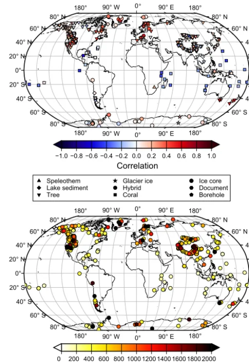
The PAGES 2k Consortium has compiled a global dataset of proxy temperature records. Records were assembled by ex-perts to represent the evolution of temperature over the last 2000 years. Quantitative criteria for record length, resolu-tion, and other factors were devolved to select a large dataset that can be culled to address a wide range of research ques-tions (http://www.pages-igbp.org/ini/wg/2k-network/intro). The first version of this dataset, containing 511 proxy records, was used to generate temperature reconstructions for seven continental-scale regions using various reconstruc-tion methods (PAGES2K Consortium, 2013). It has since been updated and expanded to include marine records and additional metadata (PAGES2K Consortium, 2017). Some records in the 2013 version were excluded because of more stringent selection criteria, which have now been applied more uniformly across regions. We use version 1.9.0 of this dataset, the predecessor to the slightly revised upcoming ver-sion 2.0.0, which will shortly be published (PAGES2K Con-sortium, 2017). Thus, the version used herein represents an intermediate snapshot between versions 1 (PAGES2K Con-sortium, 2013) and 2 (PAGES2K ConCon-sortium, 2017). In to-tal, 682 records are included from 640 terrestrial and ocean locations (Fig. 1). The records belong to 10 types of proxy archives and vary in time resolution and record duration, the majority of them being tree rings (61 %), with assumed
an-180° 180°
90° W 90° W
0° 0
90° E 90° E
180° 180°
80° S 80° S
60° S 60° S
40° S 40° S
20° S 20° S
0° 0°
20° N 20° N
40° N 40° N
60° N 60° N
80° N 80° N
−1.0 −0.8 −0.6 −0.4 −0.2 0.0 0.2 0.4 0.6 0.8 1.0 Correlation
Speleothem Glacier ice Ice core Lake sediment Hybrid Document
Tree Coral Borehole
180° 180°
90° W 90° W
0° 0°
90° E 90° E
180° 180°
80° S 80° S
60° S 60° S
40° S 40° S
20° S 20° S
0° 0°
20° N 20° N
40° N 40° N
60° N 60° N
80° N 80° N
0 200 400 600 800 1000 1200 1400 1600 1800 2000 No. of years
°
Figure 1.Top: pointwise correlation between the raw proxy series in the PAGES-SEL network and the SAT in the infilled HadCRUT4 dataset during the period 1911–1995. Each type of proxy is indi-cated with a different symbol. Bottom: number of years in which each record contains valid data, i.e. lighter colours indicate shorter records.
nual resolution. Unfortunately, not all proxies span the full period, as shown in the bottom map in Fig. 1, which depicts the number of years where each proxy does not contain miss-ing values within the period 1–2012. For further details about the database, especially regarding the nature and temporal evolution of data availability, we refer to PAGES2K Con-sortium (2017). The records with lower time resolution are interpolated to emulate annual resolution, and seasonally re-solved proxies are also processed to remove the annual cycle. This dataset is hereafter referred to as PAGES-FULL.
a statistically significant correlation with regional tempera-tures. We use the regional plus FDR (false discovery rate; Ventura et al., 2004) screening from PAGES2K Consortium (2017). This procedure selects only those proxy records with significant (p <0.05) grid cell correlations within a search radius of 2000 km and corrects for FDR. This screening re-duces the redundancy of records in areas where they clus-ter, particularly western North America and the Himalayas (Fig. 1), but also removes records from areas where the proxy density is sparse. This subset consists of just 197 records. Al-though the influence of using different subsets is addressed in Sect. 6, most of the analysis hereinafter is based on the PAGES-SEL subset.
2.3 Model simulations
The AM method requires a pool of plausible SAT fields to be used for the search of analogues. The size of this pool is cru-cial, as it needs to cover as many potential climate situations as possible that might have occurred over the Common Era. To account for this, we use an ensemble of ESM simulations, i.e. the simulations of the last millennium within the frame of the PMIP3 initiative (Braconnot et al., 2012). This ensemble is part of the Coupled Model Intercomparison Project Phase 5 (Taylor et al., 2012, CMIP5) and is produced with different state-of-the-art models that are also used in the assessment of future climate change (IPCC, 2013). The heterogeneity of this ensemble (different parameterisations, components in-cluded, etc.) is beneficial for this application since it allows the analogues to be drawn from a wide range of the spec-trum of plausible climate situations, each of them consis-tent within their own model physics. Although different in some details, all models agree in many fundamental aspects of the temperature evolution over the Common Era. They are fully coupled ocean–atmosphere general circulation models run with similar spatial resolution. Furthermore, the length of the simulations and the forcings implemented is similar, although not entirely consistent across the ensemble (Bra-connot et al., 2012; Schmidt et al., 2012; Taylor et al., 2012). In total, 16 simulations are considered from seven ESMs, re-sulting in a pool size of 18 327 years.
3 Methods
3.1 Calibration of the reconstructions
The PAGES 2k datasets consist of a network of raw, uncal-ibrated proxies. Thus, using this dataset in the AM method requires a prior calibration of the proxy series to tempera-ture that can be compared to the modelled temperatempera-ture in the search for analogues. Such calibration is a complex task since different proxies respond to temperature in a different fash-ion, and their relationship is contaminated by an unknown and different level of non-climatic noise. Furthermore, dif-ferent proxies span difdif-ferent periods, which leads to a dataset
populated with a number of missing values that vary through time. These drawbacks require a simple method capable of handling this heterogeneity. It should produce a network of reconstructed temperature records that preserves the largest fraction possible of the climate-related variability. Thereby, a simple univariate linear regression model is employed to deduce a statistical relationship between each proxy and the SAT. The regression is calculated against the closest grid point in the HadCRUT4 dataset during an overlapping pe-riod. This fit is performed for each location independently. The regression parameters estimated during the calibration period are then used to obtain a local SAT reconstruction.
The period 1911–1995 is used for the calibration, thereby avoiding the use of the full observational record, and set-ting some observational data aside for the validation of the reconstruction. Figure 1 shows the correlation between the observations and the raw proxy series during the calibra-tion period. The correlacalibra-tion ranges between−0.56 and 0.63, with 65 % of values with an absolute value below 0.2. Al-though the correlation is modest, it is important to note that these proxies have been carefully selected by experts accord-ing to their demonstrated ability to reflect temperature vari-ations with respect to the choice of the calibration period (PAGES2K Consortium, 2017). Furthermore, these correla-tion values are robust with respect to the choice of calibracorrela-tion period. Various periods have been tested, including the use of the whole period, and differences are hardly appreciable (not shown).
3.2 The AM as reconstruction technique
The AM was first introduced in the 1970s for weather fore-casting (Lorenz, 1969). Recently, it has been implemented in a variety of applications in climate research, from hurri-cane prediction (Sievers et al., 2000; Fraedrich et al., 2003) to downscaling (Zorita and von Storch, 1999) and upscaling Schenk and Zorita (2012) techniques. For the interest of this study, the suitability of this technique to generate CFRs has been recently demonstrated for temperature (Franke et al., 2010) and precipitation (Gómez-Navarro et al., 2014) for Eu-rope. Although the method is explained elsewhere, we briefly outline its key ideas here, following the notation by Gómez-Navarro et al. (2014).
The algorithm requires a set of observations of the mul-tivariate predictand T(t) available over some time t, with concurrent observations of a multivariate predictorP(t). This predictor shall also be available at timet0where no
observa-tions of the predictand, the target field variable, are available. The basic idea of the AM is that the value of these unknown T(t0) can be approximated by a known value ofT(t) if the
predictorsP(t) andP(t0) at the target timet0and a timetin
members of the pool by using a metric:
1(ti)=dist(P(t0),P(ti)), ∀i∈pool. (1)
The element in the pool with the smallest1(ti) is called the
analogue,P(eti). Thereby, the reconstructed predictand is de-fined as the value of the predictand at the analogue point in time, which minimises the metricT(t0)=T(eti).
Although the basic idea is simple, there is still flexibility for tailoring the method to fit different requirements. First, the similarity in Eq. (1) can be defined in multiple ways by using different metrics, some of which are introduced in the next sections. Additionally, the method can be set to not just select one analogue but also to identify a set of analogues (e.g. Sievers et al., 2000; Fraedrich et al., 2003). For exam-ple, theN closest analogues in the pool (in the sense of the distance given by Eq. 1) can be used to produce a weighted average:
e T(t0)=
N X
i=1
ωiT(eti), (2)
whereT(eti) denotes the predictand fields of the closest ana-logues, weighted by ωi. Again, the weighting can be
per-formed in different ways, e.g. by the distance according to the selected metric or simply by equal weights. Here, we con-sider only the casesN=1 andN=5 and set all weights to 1/N, which produces a simple average of analogues. It is important to note that the use of several analogues (N >1) filters out noise, and thus the estimation uncertainty is lower, but has the counterpart of underestimating the time variance.
3.3 Search for analogues in the real space
The measure of similarity described in Eq. (1) makes use of a distance between two patterns of temperature that has to be evaluated over the network of proxy sites. Note that such dis-tance shall be defined flexibly enough to accommodate pos-sible missing values. In this analysis we use two different metrics: correlation and RMSE.
Correlation is defined as
ρ(P(ti),P(tj))=
(P(ti)−P(ti))·(P(tj)−P(tj)) q
(P(ti)−P(ti))2(P(tj)−P(tj))2
, (3)
where the line over a vector indicates that the mean value across coordinates is computed. RMSE is defined in this no-tation as
RMSE(P(ti),P(tj))= s
(P(ti)−P(tj))2
M . (4)
Correlation is a measure of the degree of similarity of two patterns, but does not penalise two fields that may differ by a large constant value. This reduces the ability of the metric
to detect changes in the global temperature, as will be shown later. RMSE is a metric that simultaneously penalises the lack of spatial co-variability and differences in mean values. Note that this metric is equivalent, except for a multiplicative con-stant, to the Euclidean distance between the two vectorsP(ti)
andP(tj). Both metrics can be generalised in a natural way
to account for missing values in proxy sites. In that case, the summations implicit in the scalar product and in the aver-ages skip those sites, and the constantMhas to be decreased accordingly.
3.4 Search for analogues in the EOF space
As a variant, the search for analogues can be carried out in the low-dimension space expanded by the leading EOF patterns of the temperature variability. The rationale for using this transformation is that although a temperature field has many dimensions, i.e. as many as there are grid points, these grid points are strongly interdependent, thus reducing the effec-tive degrees of freedom of the phase space. Furthermore, part of this variability may be spurious and attributable to non-climate-related variability in the proxy records, i.e. noise. By decomposing the variability in the in the main modes of the field, temperature variability can be compressed into a much smaller number of independent variables, each one uncorre-lated to the others (von Storch and Zwiers, 2002). The use of EOF techniques to reduce the dimensions for the search of analogues has been explored in previous studies (Zorita and von Storch, 1999; Fernández and Sáenz, 2003).
Here, the leading modes of variability are obtained from the observational dataset HadCRUT4 (where there are no missing values). Once the leadingLpatterns that explain the desired level of variance (set to 90 % in this study) are identi-fied, the field can be approximated as the linear combination
P(t)'
L X
i=1
αi(t)EOFi, (5)
whereEOFi represent the spatial pattern and αi(t) the
cor-responding time series, which can be interpreted as the coor-dinates of a vectorα(t), whose calculation is described be-low. Thereby, the rank reduction achieved by the change of basis emerges from the fact that the vectorP(t), originally defined through M coordinates in the canonical basis, can be described on the EOF basis byL, withLM. Once the predictor and predictand at each time step are expressed as linear combination of the observed modes of variability, the AM can be applied directly in this space, with the only mod-ification that the metrics described in Eqs. (3) and (4) have to be applied using the vectorsα(ti) andα(tj), instead of the
original fieldsP(ti) andP(tj). For the EOF space we focus
on a single metric, i.e. RMSE.
Despite their apparent simplicity, the calculation coordi-nates αi(t) deserve some words of caution when working
missing values, the EOFi vectors form an orthonormal
ba-sis. In this case, each coordinateαi(t) can be easily obtained as the scalar product:
αi(t)=P(t)·EOFit, (6)
where each row is an EOF pattern and the super indext de-notes matrix transpose. However, when missing values are present in the vector P(t), such gaps have to be introduced in the vectorsEOFi. Unfortunately, this modification in the
vectors destroys their orthonormality, which implies that the former equation has to be generalised. It can be shown that the general expression is
αi(t)=P(t)·EOFti·Cov(EOF)
−1, (7)
where Cov denotes the spatial covariance matrix of theEOFi
vectors. In the particular case where they are orthonormal (e.g. when there are no missing values) the covariance matrix is the identity matrix of sizeL, and Eq. (7) becomes equal to Eq. (6).
As a final remark, the coordinatesαi(t) do not contain any
missing values, regardless of the gaps present in the origi-nal vector P(t) as missing values are implicitly taken into account in the matrix multiplication used to transform the basis. Thus, allαi(t) coordinates have the lengthL,
indepen-dent of the presence of missing values. This simplifies the definition of a distance. Still, the presence of many missing values is undesirable since it increases the uncertainty of the estimation ofαi(t).
3.5 Design of pseudo-proxy experiments
As part of the performance evaluation of the AM method, we use PPEs. These idealised experiments are profusely used in literature to assess the performance of the CFR reconstruc-tions of temperature (Smerdon, 2012, and references therein) or even precipitation (Gómez-Navarro et al., 2014). The pro-cedure extracts data from a climate simulation at a given set of locations to build a synthetic network of local pseudo-records. This synthetic dataset is used as input for the recon-struction method with the aim to recreate the reconrecon-struction procedure, and then to compare this pseudo-reconstruction with the original simulated field.
The design of PPEs may vary in complexity. The so-called perfect PPEs use the closest grid point to the location of the real proxy to extract a time series of the physical variable of interest. The synthetic reconstructions used as input therefore consist of a simple subset of the original field of the simula-tion. This is clearly an oversimplification of reality since tual local reconstructions reproduce only a fraction of the ac-tual climatic signal and include uncertain levels of noise and missing values. A more realistic approach consists of con-taminating the climate model series with a certain amount of statistical noise and number of gaps, so that the starting point of the CFR reconstructions more closely mimics real proxy data.
In this study, we select one of the simulations from the PMIP3 ensemble as a target to create the pseudo-proxies for the PPE (in particular we use the simulation with the GISS model labelled r1i1p121). We then build the pool of ana-logues from all other simulations excluding this simulation and reconstruct the target with the AM. Although the results are largely independent of the choice of model, as we in-deed demonstrate in Sect. 4.4, the rationale for this choice is that this simulation is somewhat dissimilar to the other model simulations in that it exhibits lower variability than the other models. This somewhat dissimilarity renders the exercise of reconstructing the target GISS temperature using the other models as a pool of analogues more difficult, and it therefore results in a slightly stricter test.
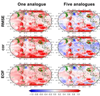
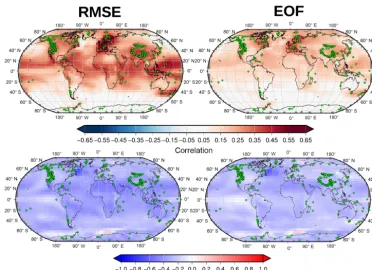
Figure 2.Pointwise correlation (calculated for the whole reconstructed period) between the original simulation and a reconstruction based on perfect pseudo-proxies. The maps show the results when three different metrics are used for the search of analogues (by rows), as well as when different numbers of analogues are combined to draw the reconstruction (by columns). Green diamonds indicate the location of the pseudo-proxies employed, based on the PAGES-SEL network.
4 Evaluation of the AM in PPEs
In this section, only PPEs are used to evaluate the perfor-mance of the AM to reconstruct global annually-resolved temperature. In all cases the full PMIP3 ensemble has been considered by leaving out one simulation, and the proxies’ locations are based on the PAGES-SEL network, as described in Sect. 3.5.
4.1 NoNoise PPE
Figure 2 shows the pointwise correlation maps (calculated for the full reconstructed period) between the original sim-ulation and the pseudo-reconstructions based on perfect pseudo-proxies with one and five analogues for a similar-ity measure based on RMSE, correlation, and RMSE in the EOF space. All methods tend to produce positive correla-tions, which is indicative of the ability of the reconstruc-tion method to recover the original variability based on a limited number of locations. Still, there are large differences among the different settings. The reconstruction based on the metric of correlation is less reliable than the one based on
devia-Figure 3.As in Fig. 2, but for the logarithm of the ratio of the standard deviation of the reconstruction and the original simulation. Red (blue) shading depicts areas where the reconstruction overestimates (underestimates) variability.
tions in the reconstruction and the simulation is presented. Overall, all reconstructions tend to preserve, and even over-estimate, the original variability well. This is a result of the lower variability in the simulation used as a target (based on the GISS model) versus the model ensemble as a whole, and thus resampling the pool of analogues tends to produce larger variability than the target. This overestimation of variability becomes strongly ameliorated when five analogues are used, as expected according to the discussion above.
Spatially, the performance, measured by the pointwise cor-relation in Fig. 2 is quite homogeneous, despite the unequal distribution of the proxies and especially despite the smaller number of proxies in the Southern Hemisphere. Within the Northern Hemisphere, the area where the reconstruction is less accurate is clearly the North Atlantic, which stands out across all reconstructions. In this sense, the EOF-based re-construction seems more robust since it does not present the slight negative correlations that appear near the North At-lantic, Caribbean Sea, and Sahara. The areas south of 40◦S show low correlations, which can be clearly associated to the lack of proxies that provide information for the reconstruc-tion. Regarding variability, the spatial structure is coherent across methods. Still, the strong underestimation of variance
in all reconstructions in the western North Atlantic is no-table. This underestimation can be directly linked to strong variance in the simulations used as a target (not shown). The consistency of these deficiencies demonstrates how the AM method is always constrained by the quality of the data used as a pool for the analogues search. In this case, the features observed in the target field are not shared across models, which leads to the inability of the method to find suitable analogues that capture certain features.
Based on the results that emerge from Figs. 2 and 3, the rest of the analysis focusses solely on the reconstructions car-ried out with the search of analogues in the real space and based on RMSE similarity (hereafter RMSE-AM) and the search of analogues in the EOF space (hereafter EOF-AM). Similarly, only reconstructions using an average of five ana-logues are discussed. However, although not shown, the anal-ysis has been carried out with all combinations of settings, and significant deviations from the results expected from the discussion above are highlighted.
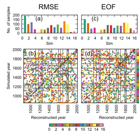
frequently, and whether there is a strong relationship between the year being reconstructed and the year that corresponds to the closest analogue. This is shown in Fig. 4, where the num-ber of times each model has been selected is shown for each method (panels a and c). All models across the pool are se-lected at some point in the reconstruction (with the exception of model number 5, which is the model explicitly excluded for being the target of the PPE). Still, some models are more frequently selected than others. Numbers 1 and 13 are overall the most frequently chosen in both methods and correspond to the BCC and the IPSL models, respectively. Conversely, models 15 and 16 are the less frequently chosen models and correspond to two realisations of the MPI model. It is worth noting that the other simulations with the GISS model (num-bers 4 to 11) are not selected more frequently than the rest of models, despite being simulations of the same model as the target. This is indicative of the ability of the search algo-rithm to identify similarities in the spatial patterns regardless of particular model features, and this supports the robustness of the reconstructed fields with respect to the biases present in some models. Thin black lines denote the occurrence of se-vere volcanic activity and are aimed at facilitating the iden-tification of relationships between this external forcing and year selection. It turns out however that the method selects analogues independently from this factor. Similarly, there is no strong one-to-one relationship between the simulated and reconstructed years, i.e. simulated modern (or earlier) years are not necessarily selected to reconstruct recent (or earlier) years (see scatter dots in panels b and d). This is indicative of the sufficiently large amount of variability contained in the pool, which, thanks to the amount of internal variability provided by the various simulations, is able to provide ana-logues independently of the model year. The only signal of a temporal link between the targets and their analogues ap-pears as a clustering of modern simulated years that are used as analogues for years within the 20th century (see the clus-tering of dots in the top right corners in panels b and d). This is attributable to the effect of recent warming of the indus-trial period, i.e. warm years appear more frequently, and they are preferably found during the last centuries of the pool of simulations.
4.2 R0.5 PPE
This section explores the performance loss when noisy pseudo-proxies are used to mimic the effect of non-climate-related variability in real proxy data. As outlined above, the noise consists of additive white noise and the introduction of missing values that mimic the temporal distribution of miss-ing values present in the PAGES-SEL network. Note that, for the sake of brevity, the analysis hereafter is limited to the RMSE-AM and EOF-AM methods for analogue search, al-though the other methods have been explored and the results are consistent with the former section, i.e. the RMSE met-ric outperforms correlation as a measure of distance between
0 50 100 150 200
0 2 4 6 8 10 12 14 16
No. of samples
Sim
0 2 4 6 8 10 12 14 16
Sim no.
0 50 100
150200
0 2 4 6 8 10 12 14 16 Sim
RMSE
EOF
(a) (c)
1000 1200 1400 1600 1800 2000
1000 1200 1400 1600 1800 2000
Simulated year
Reconstructed year
(b)
1000 1200 1400 1600 1800 2000
Reconstructed year
(d)
0 2 4 6 8 10 12 14 16
Figure 4.Selection of analogues used to carry out a perfect PPE.
Bars in panels(a, c)indicate the number of times the analogue has
been taken from each of the 16 models. The points in panels(b,
d)indicate the relationship between the reconstructed year (xaxis)
and the model (colour) and simulated year (yaxis) used as analogue
for the reconstruction. Black horizontal and vertical lines show the timing of major volcanic eruptions according to Sigl et al. (2015).
Panels(a, b)correspond to the reconstruction based on RMSE and
(c, d)based on Euclidian distance in the EOF space.
analogues. Similarly, only the reconstruction obtained as an average for the five best analogues is discussed since the one-and five-analogue versions differ in the bias–variance trade-off described in the perfect scenario context in the previous section.
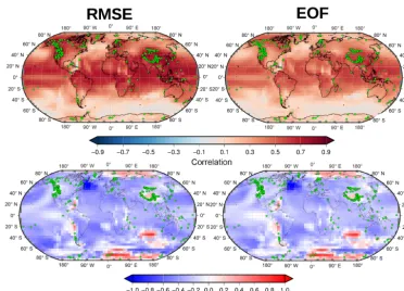
Figure 5.Similar to Figs. 2 and 3 but for realistic PPE. Top (bottom) row indicates the correlation (ratio of standard deviations) between the original simulation used as a target and the reconstructions obtained selecting analogues from the PMIP3 pool.
at a given location can be, to a great extent, recovered by the reconstruction method through the use of nearby infor-mation and by the spatial coherence of the climate field. This recovery of degraded information gives confidence about the CFR methods in general, and in the AM in particular, and suggests that the use of a large network of independent prox-ies can overcome, to a certain extent, the problems derived from the use of noisy local reconstructions. The two maps in the lower row depict the ratio of standard deviation in the reconstruction and the simulation on a logarithmic scale. Both figures are hardly distinguishable (spatial correlation 0.97 and averaged bias of −0.02) and coherently point out how the reconstruction recovers about 80 % of the original variance independently from the particular method (the log-arithm of the ratio averages −0.1 and −0.8 for RMSE and EOF, respectively). The loss of variance with respect to the NoNoise PPE is particularly strong in the western North At-lantic. This underestimation of variance disappears and even becomes an overestimation of variance when just one ana-logue is considered (not shown). However, this variant of the method presents lower temporal correlation (not shown), as the correlation–variance trade-off is always present across experiments.
The results obtained with the experiments where red in-stead of white noise is added to the original series resemble those shown in Fig. 5 and are not shown due to the great similarity with the figures corresponding to white noise. All metrics evaluated indicate that the performance of the
recon-struction is indistinguishable when either white or red noise is considered. Therefore, the presence of memory in prox-ies seems to play a secondary role in the performance of the AM and does not noticeably degrade the output of the re-construction. Note that this result agrees with previous find-ings in similar studies that were aimed at the reconstruction of precipitation (Gómez-Navarro et al., 2014). The effect of red-noise pseudo-proxies has been tested in previous stud-ies in the context of regression-based methods and the com-posite plus scaling method (von Storch et al., 2008), where it was found that, in the case of regression methods, red-noise pseudo-proxies lead to a stronger underestimation of past variability than white-noise pseudo-proxies. However, the influence on other measures of skill that do not rely on the amplitude of variations, like correlation, has so far not been investigated. It is therefore reassuring that the AM does not lead to either an additional reduction in past variations or to a loss of correlation skill.
4.3 RProxy PPE
Figure 6.As in Fig. 5 but for the hyperrealistic PPE in which the correlations equal the values obtained during the proxy calibration, i.e. Fig. 1.
the ability of the AM method to reconstruct the original sim-ulation. The correlation between the pseudo-reconstruction and the target is especially reduced in the tropics and North America, locations where the skill obtained in more simple PPEs is very remarkable, and perhaps overestimated under the light of this analysis. There are however areas where the correlation is still well preserved, such as in Europe, cen-tral Asia, and the western Pacific. A striking finding with re-spect to the former case is the large difference between the RMSE-AM and EOF-AM methods. Although both methods deal with the same amount of uncertainty, the former clearly outperforms the latter regarding its ability to reproduce the temporal evolution in the target, despite the addition of noise and missing values. Still, the spatial structure of correlation is very similar in the RMSE-AM variant, and in particular the method remains able to deliver performance in regions with poor proxy coverage. Regarding the preservation of variance, both methods exhibit the same underestimation of variance, which stems from the averaging over five analogues, and is absent in both cases when only one analogue is used to re-construct (not shown). Thus, both methods behave similarly regarding the replication of variance.
Based on the results of these PPEs, we conclude that the RMSE-AM method is overall the most reliable since its per-formance is more robust across the experiments and analyses we have carried out.
4.4 Other simulations as targets
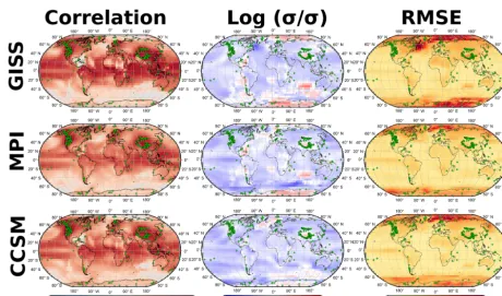
col-Figure 7.Correlation (left), logarithm of the ratio of the standard deviations (middle), and RMSE (right) between the target SAT and the pseudo-reconstructed SAT based on a PPE with additive white noise as in Sect. 4.2. All reconstructions use the same AM setup based on searching analogues that minimises RMSE and then averaging the five closest analogues. The only difference across rows is the model used as a target for the PPE: GISS (top map, equivalent to Fig. 5), MPI-ESM-P (middle), and CESM4 (bottom).
umn) are also similar in both cases. The RMSE tends to be higher in the GISS case, confirming our initial assumption that the variability in the GISS model stands slightly out of the ensemble of models, though not dramatically. The RMSE is higher in the polar regions, where it may attain values of the order of 2–3 K, and rather uniform and lower values around 0.5 K around the rest of the globe. There is a remark-able difference between both cases in the western North At-lantic, where the GISS case displays rather large values of the RMSE that are not seen in the MPI-ESM-P case, for which there is no clear explanation at this point. Regarding the preservation of variance (see middle column in Fig. 7), there are small regional deviations, which seem model-dependent, although the main picture that stands out in all the three cases is that the reconstruction using five analogues leads to a slight but generalised loss of variance. Therefore, the main conclu-sion we can draw from the analysis above is that the choice of simulation as a SAT target does not largely affect the per-formance of the AM in reconstructing global SAT, and the conclusions drawn from the analysis of the GISS model used as a target can be safely extended to other models.
5 Reconstruction of the observational period
In this section, the ability of the reconstruction method is ex-plored using real proxies to reconstruct the observed
tem-perature field in the period 1850–2012. For this, a selection of the PAGES-SEL network during the period 1850–2000 is extracted and calibrated during the 1911–1995 period against the infilled HadCRUT4 observational dataset in the way de-scribed in the Sect. 3. The series obtained after calibration are used as input for the RMSE-AM and EOF-AM variants of the AM, and the output is compared to the original obser-vations, with the aim of establishing the performance of the reconstruction.
spa-Figure 8.Similar to Figs. 5 and 6, but for a reconstruction of observations based on a calibration of proxies in the period 1911–1995. The correlation is calculated for the period 1850–2010.
tially homogeneous noise (Figs. 2 and 5, respectively). This lower temporal correlation may be due to two reasons. One is that the level of noise employed in the first realistic PPE, in-spired by its application in similar studies (von Storch et al., 2008; Smerdon, 2012; Gómez-Navarro et al., 2014), is an underestimation. Indeed, the pointwise correlations between the observed temperature and the proxies during the calibra-tion period range between−0.56 and 0.63, with an average of 0.06, which would suggest a higher level of noise in the real world than in the PPE. However, a second reason could orig-inate in a deficient simulation of the typical temperature pat-terns found in the real world. These low correlations impose an upper limit to the temporal evolution that the calibrated series are able to represent. This can be seen more clearly when comparing Figs. 6 and 8, where especially the RMSE-AM method exhibits a very similar spatial pattern and values (again, recall that the PPE is again in disadvantage as corre-lations in Fig. 6 are calculated for the whole Common Era, including early periods more densely populated with miss-ing values). Note that these figures correspond to very differ-ent datasets (a PPE versus a real reconstruction of an obser-vational dataset), although by construction of the PPE they have the spatial proxy network and the correlation between the proxy and the corresponding local SAT series during the instrumental period in common.
The reconstructions of the temperature in the observa-tional period produce overall positive correlations with the real temperatures. These correlations match fairly well with
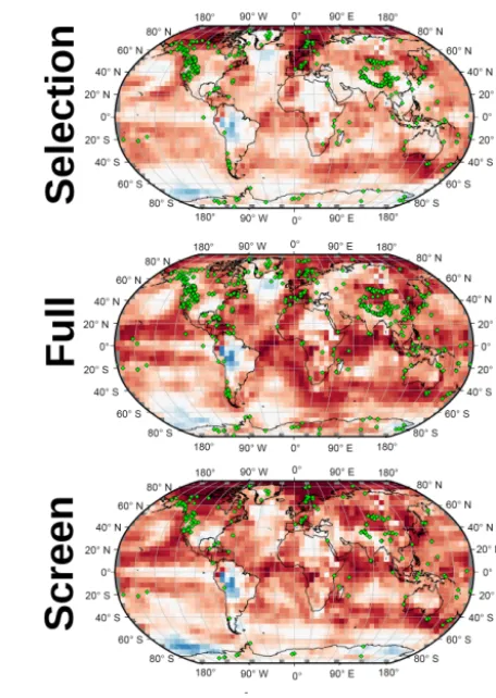
pro-Figure 9. Correlation maps similar to Fig. 8 for the RMSE-AM variant of the AM method. The three maps depict the result obtained using each of the three variants of the PAGES 2k network described in Sect. 2.2. In all cases the green symbols indicate the location of the proxies employed in the reconstruction.
vides an example of unavoidable bottleneck of the AM. It is however worth noting that an alternative or complementary explanation for the differences in variability between obser-vations and simulations in the Arctic regions could be caveats in the former. This is due to the fact that as outlined in the dataset decryption above, observations in the high Arctic are not real but are infilled using extrapolation techniques that might introduce variance overestimation.
6 The role of spatial distribution of proxy sites
The reconstruction performance may also depend on the proxy network used. Therefore, we assess the impact of slightly different proxy networks on the reconstruction, us-ing the PAGES-SEL, PAGES-FULL, and PAGES-SCREEN networks described above. The observational period serves as an example.
The correlation maps between the observations in the pe-riod 1850–2000 and the different RMSE-AM reconstructions
based on these networks are shown in Fig. 9, where the slightly different distribution of the proxies is also shown. Using the original PAGES-FULL network generally im-proves the pointwise correlation of the reconstruction com-pared to the PAGES-SEL case (recall that this network con-tains 682 instead of 514 records). This is especially so in equatorial and sparsely covered areas, indicating that the ad-dition of a few records, even when they do not provide real annual resolution or when they contain significant numbers of missing values, can have noticeable positive effects on the reconstruction. A striking result is that the PAGES-SCREEN network provides remarkable performance, despite that it just contains 197 records. This suggests that the accumulation of redundant proxies in certain areas, such as North America or China, may have a counterproductive effect in the reconstruc-tion performance. This is a somewhat counter-intuitive result since the screening of the network produces a reduction in the available information. However, our results indicate that the performance is to a large extent preserved, probably because the screened network contains fewer proxies that exhibit low correlations with the instrumental temperature. The combi-nation of the latter two results supports the argument that the best possible network would ideally have a global but also a very homogeneous coverage, making the total number of records of secondary importance.
Figure 10 shows the temporal evolution of the globally averaged SAT in the HadCRUT4 dataset and the RMSE-AM reconstructions with one and five analogues using each of the proxy networks described previously. This figure ad-ditionally illustrates the reconstruction performance, and is complementary to the correlation maps discussed so far. All time series reproduce the global warming captured by ob-servations remarkably well, including the short cooling pe-riod during the 1960s. The differences between the different settings of the method are minor and do not affect this gen-eral good agreement, indicating that the long-term variability can be reproduced with confidence regardless of the network used to reconstruct the climate variability.
7 On the estimation of reconstruction uncertainties
illustra--0.8 -0.6 -0.4 -0.2 0 0.2 0.4 0.6 0.8 1 1.2
1860 1880 1900 1920 1940 1960 1980 2000
Global SAT anomaly (C)
Year PAGES-SEL N = 1
PAGES-SEL N = 5 PAGES-FULL N = 1 PAGES-FULL N = 5 PAGES-SCREEN N = 1 PAGES-SCREEN N = 5 HadCRUT4
Figure 10.Time series of globally averaged SAT anomalies with respect to the period 1961–1990. The bold black line represents the infilled HadCRUT4 dataset, whereas colours indicate six
recon-structions based onN=1,5 in Eq. (2) using the RMSE-AM
ver-sion with the three variants of the PAGES 2k network described in Sect. 2.2.
tion, let us consider the well-known case of a simple univari-ate regression model (see for instance von Storch and Zwiers, 2002).
T =Tm+(P−Pm)α+, (8)
whereT andP denote temperature and proxy, respectively;
TmandPmdenote their mean values;αis the regression co-efficient; andis the error term. The uncertainty in the esti-mation ofT givenP has two main sources. One is related to the amplitude of the unresolved variance, given by the stan-dard deviation of . However, the other main source is the uncertainty in the estimation of α; let us denote it asδ(α). As can be demonstrated within the linear regression theory, this second contribution is approximately proportional to the product (P−Pm)δ(α). Therefore, for values ofP in the
mid-dle of the range of the predictor, the main contribution is the amplitude of, whereas for values ofP far away fromPm,
the main contribution becomes (P−Pm)δ(α).
In a similar way, in the application of the AM there are two main contributions. One would be the amplitude of the error term, i.e. the deviations between the actual and predictedT, assuming that the model analogue is perfect. This contribu-tion is analogous to the unresolved variance, i.e. the variabil-ity inT at a certain point that cannot be solely determined by the given temperatures at the proxy locations. A second con-tribution to uncertainty is the identification of the analogue it-self. Unfortunately, the situation in the AM is more complex than in the case of simple univariate regression. For target patterns where good analogues can be easily be found, this contribution will be very small. In general, and since we use a large pool for the analogue search, it can be assumed that for proxy patterns that are around the mean, the AM is gen-erally able to find good analogues within the pool. However, for proxy patterns well beyond the range of the pool, where
no good analogues can be found, the uncertainty cannot be easily quantified. The reason for this is that such an estima-tion would require an analytical model, being the counterpart of the regression model outlined above. Unfortunately such a frame model, able to carry out some sort of analogue extrap-olation model that would allow the estimation of a range of the predicted variable in ranges where no good analogue of the predictor exists, has not been developed yet. Therefore, for targets well beyond the analogue pool, this contribution to uncertainty would be the largest, although unknown. Note that this situation is, to some extent, similar to pollen-based reconstructions using the analogue method (Overpeck et al., 1985). When the pollen record shows a pattern that is not present in the current pollen distribution, the climate recon-struction and its uncertainty are virtually impossible to es-timate. In this regard, new mathematical developments are required to settle this issue.
Under light of the former discussion, in this paper we have estimated just the uncertainty arising from one of the two contributions discussed above, i.e. the variability inT at a certain point that cannot be solely determined by the given temperatures at the proxy locations. To do so, we do opt by computing the standard deviations of the residuals (re-constructions minus target). For this computation, we try to mimic the situation that researchers face in real reconstruc-tions, where the observed temperature field over a reference period would be known, so that the residuals (deviations be-tween observations and reconstructions) and their standard deviation can be computed. To simulate as closely as possi-ble this situation, we compute the standard deviation of the differences using the 1850–2005 period, instead of the whole GISS r1i1p1 simulation.
divid-Figure 11.Left column: local standard deviation of the residuals (GISS r1i1p1 annual mean SAT minus pseudo-reconstructed SAT) over the period 1850–2005. Top: using a pseudo-proxy network with as many missing values as the PAGES-SEL network in 1500 (257 records). Bottom: using the maximum number of pseudo-proxy locations of the same network, which happens in 1949 (514 records). Right column: same as left column, but normalised by the standard deviation of the target. The precise locations of the pseudo-proxies are indicated with green symbols.
ing by the standard deviation of the target. Quite remarkably, the number of proxies has little influence on the intensity and distribution of errors. This is in good concordance with the results discussed in Sect. 6 and once again demonstrates the secondary role of the absolute number of proxies, as a grow-ing number of proxies sometimes increases redundancy with-out providing independent source of insight.
8 Conclusions
This study presents a framework to carry out global CFRs using the AM based on a pool of the PMIP3 ensemble simu-lations (Taylor et al., 2012). Although the application of the method has been previously employed to carry out European reconstructions of temperature (Franke et al., 2010) and pre-cipitation (Gómez-Navarro et al., 2014), the validity of this method to accomplish a global temperature field reconstruc-tion has not been addressed so far. This is a relevant test since the large dimensionality of the problem poses concerns about the suitability of available simulations to provide a large-enough pool of situations from which to draw analogues. This study is also novel in being one of the first analyses that benefits from the PAGES 2k proxy network (PAGES2K Consortium, 2017). In this sense, this work takes advantage of the most recent developments in both the climate model and reconstruction communities (PAGES 2k-PMIP3 group, 2015) and represents an example of the power of exercises blending both approaches to gain insight into climate vari-ability within the Common Era.
A number of variations in the method are presented here since the AM critically depends on the metric used to iden-tify analogues (normally a distance measure between the ana-logue and the target). Testing different metrics shows that the RMSE, which is equivalent to the Euclidean distance, is more suitable than correlation since it penalises deviations in global averages. The search of analogues in the real space, as well as the one expanded by the leading EOFs that explain 90 % of the total variance, has been explored. Although the EOF version is in principle better suited for the search of ana-logues due to the reduction in dimensionality of the problem, our results indicate that the search in the real space provides the best results with a consistent performance across the var-ious tests carried out. Furthermore, it has the added value of a slightly lower computational cost.
The inclusion of a spatially constant amount of noise in the more realistic pseudo-reconstructions does not dramati-cally affect the CFR performance, supporting the robustness of the method and the ability of the network of proxies to re-tain the variability in the global mean temperature, in spite of local noise. In particular, there is no difference in the perfor-mance between the PPE when either white or red noise with a decorrelation time of 5 years is used. This indicates that the AM is not sensitive to the presence of memory in the local proxies. Still, there is a large difference in the performance obtained with actual proxies and that achieved in PPEs with degraded pseudo-proxies. This difference suggests that the amount of noise might have been underestimated in previous studies based on PPEs (e.g. von Storch et al., 2008; Gómez-Navarro et al., 2014), and lower signal-to-noise ratio shall be employed in realistic PPEs. This is confirmed by our analysis through a more realistic PPE configuration, where the level of noise depends on the proxy site to mimic the one derived from the calibration of real proxies.
Many statistical climate reconstruction methods tend to underestimate climate variability, especially those based on linear methods. The AM is an exception since the variabil-ity in the reconstruction is provided by that of the pool of analogues. Although this might be seen as an advantage, it has the problem that systematic biases in the pool are trans-ferred to the reconstruction. This is particularly the case with the PMIP3 ensemble, which exhibits a reduced variability in the Arctic compared to the infilled observations that might become a prominent drawback in all reconstructions evalu-ated here. The AM can be adjusted by varying the number of proxies used to draw an analogue. If more than one ana-logue is selected and averaged to generate the anaana-logue, the correlation is increased, but it has the counterpart of reducing variability. This bias–variance trade-off is not unexpected, as it is a common phenomenon that appears recurrently in all branches of statistics.
The sensitivity of the CFR to various slightly different ver-sions of the proxy network has also been evaluated. The skill of the reconstruction does not critically depend on the total number of records. Instead, it is more strongly affected by their spatial distribution. In this sense, including redundant proxies that cluster in some areas does not always have a beneficial effect since they do not provide new information but may bias the search of analogues towards those areas at the coast, producing less accurate reconstructions in areas not covered as well by proxies.
The AM produces climate reconstructions that are clearly not free of uncertainties and errors. However, a full treatment and characterisation of such errors is not tackled in this study, as such an assessment would require new mathematical de-velopment that is beyond the scope of this article. Still, we investigate a part of such uncertainty, namely the part at-tributable to the unresolved variance. We characterise it by computing the standard deviation of the residuals using two different networks of pseudo-proxies and demonstrate how
such uncertainty is bounded by 1–2 K in the polar regions, with smaller uncertainty in tropical regions.
Finally, we would like to remark that as the performance of the AM has been evaluated mostly through PPE in this pa-per, and although we have tried to mimic the limitations of actual data, we note that our estimation of skill can be op-timistic, especially in the Southern Hemisphere. This is due to the fact that reconstructions show less homogeneity back through time than the models that are used in this study. For instance, it has been reported that the co-variability between both hemispheres is larger in models than in current recon-structions (Neukom et al., 2014; PAGES 2k-PMIP3 group, 2015).
We conclude that the AM is a useful tool able to yield skill-ful results in CFRs of past climate. It has particular features compared to more commonly used CFR techniques, e.g. it is a non-linear method that does not require the calibration of an underlying statistical model. Thus, the method may comple-ment more traditional approaches, providing additional in-sight about past climate variability and allowing the assess-ment of the robustness and weaknesses of other methods.
Data availability. Three independent datasets were used for the analysis in this study. The HadCRUT4 dataset is described in the references provided in Sect. 2.1 and is available under https://www. metoffice.gov.uk/hadobs/hadcrut4. The model simulations used as a pool of analogues were downloaded from the Earth System Grid Federation: https://esgf-data.dkrz.de/search/cmip5-dkrz/. Note that all available “past1000” simulations were selected. Finally, the PAGES 2k temperature proxy database (currently version 2) is available under https://figshare.com/s/d327a0367bb908a4c4f2. All programs and scripts used to perform the analysis, as well as the intermediate datasets, e.g. the pseudo-proxy reconstructions, are available upon request.
Competing interests. The authors declare that they have no con-flict of interest.
Acknowledgements. This is a contribution to the PAGES 2k Net-work. Researchers of the PAGES 2k Consortium are thanked for creating and releasing the database of proxy data and metadata. Julien Emile-Geay and Nick McKay provided the data files of the PAGES 2k database and the PAGES-SCREEN dataset used herein. Darrell Kaufmann provided inputs on the data section.
We acknowledge the World Climate Research Programme Work-ing Group on Coupled ModellWork-ing, which is responsible for CMIP, and we thank all the climate modelling groups for producing and making available their model output.
(project 20022/SF/16). Christoph C. Raible acknowledges support from the Swiss National Science Foundation. Raphael Neukom is supported by the Swiss NSF grant PZ00P2_154802.
The authors would like to thank the reviewers for the time devoted to carefully reading the paper and providing very useful insight.
Edited by: J. Guiot
Reviewed by: E. Boucher and one anonymous referee
References
Bhend, J., Franke, J., Folini, D., Wild, M., and Brönnimann, S.: An ensemble-based approach to climate reconstructions, Clim. Past, 8, 963–976, https://doi.org/10.5194/cp-8-963-2012, 2012.
Braconnot, P., Harrison, S. P., Kageyama, M., Bartlein,
P. J., Masson-Delmotte, V., Abe-Ouchi, A., Otto-Bliesner, B., and Zhao, Y.: Evaluation of climate models using palaeoclimatic data, Nature Climate Change, 2, 417–424, https://doi.org/10.1038/nclimate1456, 2012.
Cook, E. R., Woodhouse, C. A., Eakin, C. M., Meko, D. M., and Stahle, D. W.: Long-Term Aridity Changes in the Western United States, Science, 306, 1015–1018, https://doi.org/10.1126/science.1102586, 2004.
Fernández, J. and Sáenz, J.: Improved field reconstruction with the analog method: searching the CCA space, Clim. Res., 24, 199– 213, 2003.
Fraedrich, K., Raible, C. C., and Sielmann, F.: Analog Ensem-ble Forecasts of Tropical Cyclone Tracks in the Australian Re-gion, Weather Forecast., 18, 3–11, https://doi.org/10.1175/1520-0434(2003)018<0003:AEFOTC>2.0.CO;2, 2003.
Franke, J., González-Rouco, J. F., Frank, D., and Graham, N. E.: 200 years of European temperature variability: insights from and tests of the proxy surrogate reconstruction analog method, Clim. Dynam., 37, 133–150, https://doi.org/10.1007/s00382-010-0802-6, 2010.
Gómez-Navarro, J. J., Werner, J., Wagner, S., Luterbacher, J., and Zorita, E.: Establishing the skill of climate field reconstruc-tion techniques for precipitareconstruc-tion with pseudoproxy experiments, Clim. Dynam., 45, 1395–1413, https://doi.org/10.1007/s00382-014-2388-x, 2014.
Goosse, H., Renssen, H., Timmermann, A., Bradley, R. S., and Mann, M. E.: Using paleoclimate proxy-data to select op-timal realisations in an ensemble of simulations of the cli-mate of the past millennium, Clim. Dynam., 27, 165–184, https://doi.org/10.1007/s00382-006-0128-6, 2006.
Guillot, D., Rajaratnam, B., and Emile-Geay, J.: Statistical paleocli-mate reconstructions via Markov random fields, Ann. Appl. Stat., 9, 324–352, https://doi.org/10.1214/14-AOAS794, 2015. Guiot, J., Pons, A., de Beaulieu, J. L., and Reille, M.: A
140,000-year continental climate reconstruction from
two European pollen records, Nature, 338, 309–313,
https://doi.org/10.1038/338309a0, 1989.
Guiot, J., Corona, C., and Members, E.: Growing
Sea-son Temperatures in Europe and Climate Forcings
Over the Past 1400 Years, PLOS ONE, 5, e9972,
https://doi.org/10.1371/journal.pone.0009972, 2010.
Hakim, G. J., Emile-Geay, J., Steig, E. J., Noone, D., An-derson, D. M., Tardif, R., Steiger, N., and Perkins, W. A.:
The last millennium climate reanalysis project: Framework and first results, J. Geophys. Res.-Atmos., 121, 6745–6764, https://doi.org/10.1002/2016JD024751, 2016.
IPCC: Climate Change 2013: The Physical Science Basis. Contri-bution of Working Group I to the Fifth Assessment Report of the Intergovernmental Panel on Climate Change, edited by: Stocker, T. F., Qin, D., Plattner, G. K., Tignor, M., Allen, S. K., Boschung, J., Nauels, A., Xia, Y., Bex, V., and Midgley, P. M., Cambridge University Press Cambridge, UK, and New York, 2013.
Lorenz, E. N.: Atmospheric Predictability as
Re-vealed by Naturally Occurring Analogues, J.
At-mos. Sci., 26, 636–646,
https://doi.org/10.1175/1520-0469(1969)26<636:APARBN>2.0.CO;2, 1969.
Luterbacher, J., Dietrich, D., Xoplaki, E., Grosjean, M., and Wan-ner, H.: European seasonal and annual temperature variability, trends, and extremes since 1500, Science, 303, 1499–1499, 2004. Luterbacher, J., Werner, J. P., Smerdon, J. E., Fernández-Donado, L., González-Rouco, F. J., Barriopedro, D., Ljungqvist, F. C., Büntgen, U., Zorita, E., Wagner, S., Esper, J., McCarroll, D., Toreti, A., Frank, D., Jungclaus, J. H., Barriendos, M., Bertolin, C., Bothe, O., Brázdil, R., Camuffo, D., Dobrovolný, P., Gagen, M., García-Bustamante, E., Ge, Q., Gómez-Navarro, J. J., Guiot, J., Hao, Z., Hegerl, G. C., Holmgren, K., Klimenko, V. V., Martín-Chivelet, J., Pfister, C., Roberts, N., Schindler, A., Schurer, A., Solomina, O., Gunten, L. v., Wahl, E., Wanner, H., Wetter, O., Xoplaki, E., Yuan, N., Zanchettin, D., Zhang, H., and Zerefos, C.: European summer temperatures since Roman times, Environ. Res. Lett., 11, 024001, https://doi.org/10.1088/1748-9326/11/2/024001, 2016.
Mann, M. E. and Rutherford, S.: Climate reconstruction us-ing “Pseudoproxies”, Geophys. Res. Lett., 29, 139-1–139-4, https://doi.org/10.1029/2001GL014554, 2002.
Mann, M. E., Zhang, Z., Hughes, M. K., Bradley, R. S., Miller, S. K., Rutherford, S., and Ni, F.: Proxy-based reconstructions of hemispheric and global surface temperature variations over the past two millennia, P. Natl. Acad. Sci. USA, 105, 13252–13257, https://doi.org/10.1073/pnas.0805721105, 2008.
Morice, C. P., Kennedy, J. J., Rayner, N. A., and Jones, P. D.: Quantifying uncertainties in global and regional temperature change using an ensemble of observational estimates: The HadCRUT4 data set, J. Geophys. Res.-Atmos., 117, D08101, https://doi.org/10.1029/2011JD017187, 2012.
Neukom, R., Gergis, J., Karoly, D. J., Wanner, H., Curran, M., El-bert, J., González-Rouco, F., Linsley, B. K., Moy, A. D., Mundo, I., Raible, C. C., Steig, E. J., van Ommen, T., Vance, T., Vil-lalba, R., Zinke, J., and Frank, D.: Inter-hemispheric temperature variability over the past millennium, Nature Climate Change, 4, 362–367, https://doi.org/10.1038/nclimate2174, 2014.
Nicault, A., Alleaume, S., Brewer, S., Carrer, M., Nola, P., and Guiot, J.: Mediterranean drought fluctuation during the last 500 years based on tree-ring data, Clim. Dynam., 31, 227–245, https://doi.org/10.1007/s00382-007-0349-3, 2008.
Overpeck, J. T., Webb, T., and Prentice, I. C.: Quantitative inter-pretation of fossil pollen spectra: Dissimilarity coefficients and the method of modern analogs, Quaternary Res., 23, 87–108, https://doi.org/10.1016/0033-5894(85)90074-2, 1985.