Multi-timescale data assimilation for atmosphere–ocean state estimates

doi:10.5194/cp-12-1375-2016

© Author(s) 2016. CC Attribution 3.0 License.

Multi-timescale data assimilation for atmosphere–ocean

state estimates

Nathan Steiger1and Gregory Hakim2

1_{Lamont-Doherty Earth Observatory, Columbia University, Palisades, NY, USA}

2_{Department of Atmospheric Sciences, University of Washington, Seattle, WA, USA}

Correspondence to:Nathan Steiger (nsteiger@ldeo.columbia.edu)

Received: 22 July 2015 – Published in Clim. Past Discuss.: 19 August 2015 Revised: 21 May 2016 – Accepted: 27 May 2016 – Published: 24 June 2016

Abstract.Paleoclimate proxy data span seasonal to millen-nial timescales, and Earth’s climate system has both high-and low-frequency components. Yet it is currently unclear how best to incorporate multiple timescales of proxy data into a single reconstruction framework and to also capture both high- and low-frequency components of reconstructed variables. Here we present a data assimilation approach that can explicitly incorporate proxy data at arbitrary timescales. The principal advantage of using such an approach is that it allows much more proxy data to inform a climate recon-struction, though there can be additional benefits. Through a series of offline data-assimilation-based pseudoproxy exper-iments, we find that atmosphere–ocean states are most skill-fully reconstructed by incorporating proxies across multiple timescales compared to using proxies at short (annual) or long (∼decadal) timescales alone. Additionally, reconstruc-tions that incorporate long-timescale pseudoproxies improve the low-frequency components of the reconstructions rela-tive to using only high-resolution pseudoproxies. We argue that this is because time averaging high-resolution observa-tions improves their covariance relaobserva-tionship with the slowly varying components of the coupled-climate system, which the data assimilation algorithm can exploit. These results are consistent across the climate models considered, despite the model variables having very different spectral characteris-tics. Our results also suggest that it may be possible to re-construct features of the oceanic meridional overturning cir-culation based on atmospheric surface temperature proxies, though here we find such reconstructions lack spectral power over a broad range of frequencies.

1 Introduction

Paleoclimate proxies sample widely different timescales. High-resolution paleoclimate proxies such as tree rings or corals have annual or seasonal resolution, whereas lower res-olution proxies such as sediment cores can provide anywhere from annual- to millennial-scale information depending on the core and its location (Bradley, 2014). Additionally, high-resolution proxies tend to be short, and are mostly limited to the past two millennia, whereas some low-resolution proxies can reach the Cenozoic (e.g., Zachos et al., 2008). In addi-tion to the many timescales of proxies, the climate system itself varies across a large range of timescales: from atmo-spheric blocking to ocean overturning circulation to ice-age cycles. Thus, any faithful reconstruction of past climate must account for as many of these timescales, captured by both proxies and climate models, as possible.

tech-niques have few degrees of freedom on which to be cali-brated and validated if the timescale is longer than about a decade. Specific methods that have been developed with multiple timescales in mind include the time-series recon-struction methods of Li et al. (2010) and Hanhijärvi et al. (2013). Li et al. (2010) use a Bayesian hierarchical model ap-proach, while Hanhijärvi et al. (2013) use an approach based on pairwise comparisons that is particularly flexible and was used extensively, for example, in a recent high-profile pa-per that reconstructed continental-scale tempa-peratures over the common era (PAGES 2k Consortium, 2013). Space–time reconstruction methods include Guiot and Corona (2010) and Carro-Calvo et al. (2013). Guiot and Corona (2010) devel-oped a spectral analog approach, where analogs are drawn from an instrumental temperature data product, that they used to reconstruct European April–September temperatures over the past 1400 years. Carro-Calvo et al. (2013) developed a generalized neural network approach and used it to recon-struct winter precipitation in the Mediterranean over the past 300 years.

Data assimilation (DA) provides a flexible framework for combining information from paleoclimate proxies with the dynamical constraints of climate models. In principle, DA can provide reconstructions of any model variable, from sur-face temperature to sea water salinity to atmospheric geopo-tential height. Among DA techniques, we are unaware of any method specifically designed for the challenges of paleocli-mate reconstructions that incorporates proxies across an arbi-trary range of timescales. DA-based reconstructions have so far used only a single uniform timescale (e.g., Goosse et al., 2012) or have performed separate reconstructions at differ-ent uniform timescales (Mathiot et al., 2013). Traditional DA adjoint methods as applied in weather forecasting can and do include multiple timescales (Kalnay, 2003, p. 181– 184), but these timescales are very short by comparison to the timescales involved in paleoclimate. Here we develop a DA-based algorithm for space–time climate reconstructions that can assimilate proxies at any time resolution. Because of the limited time span of observational data sets, we explore the features and skill of this technique within a synthetic, pseu-doproxy framework. The ensuing pseupseu-doproxy experiments use an “offline” DA implementation, wherein prior ensem-bles are drawn from a previously run climate model simula-tion and are not integrated forward in time after each DA up-date step. This allows us to test the algorithm over long time spans, perform carefully controlled experiments, and unam-biguously define errors.

Multiproxy reconstructions can potentially overcome some limitations of single proxy reconstructions, such as fill-ing in for the missfill-ing frequency components of a particular proxy (Li et al., 2010). However, the primary, pragmatic ben-efit to incorporating proxies at multiple temporal resolutions is that more information can inform the reconstruction. By comparison with current weather observations, paleoclimate proxies are more expensive and time-consuming to gather

and their spatial distribution is far less extensive. Therefore, including any additional unbiased information should mean-ingfully improve the reconstructions. In addition, it is possi-ble that particular reconstruction methods could benefit from multi-scale proxy data. Within a coupled atmosphere–ocean DA framework, Tardif et al. (2014) suggest that assimilat-ing time-averaged observations of atmospheric variables may improve present-day estimates of ocean circulation. They ar-gue that these improvements arise from the fact that time averaging high-frequency observations improves the signal over noise in the covariance relationship between the atmo-sphere and the slowly varying ocean overturning circulation. We test this hypothesis within a paleoclimate context and as-sesses whether or not atmosphere–ocean state estimates can be improved by including proxies and climate states at mul-tiple timescales. Therefore this test goes beyond the benefit of simply being able to include more proxies in climate re-constructions.

2 Assimilation technique

Data assimilation refers to a mathematical technique of opti-mally combining observations (or within this context, proxy data) with prior information, typically from a model. The model, in this case a climate model, provides an initial, or prior, state estimate that one can update in a Bayesian sense based on the observations and an estimate of the errors in both the observations and the prior. The prior contains any climate model variables of interest and the updated prior, called the posterior, is the best estimate of the climate state given the observations and the error estimates. The basic state update equations of DA (e.g., Kalnay, 2003) are given by

xa =xb+K[y−H(xb)], (1)

whereKcan be written as

K=cov(xb,H(xb))[cov(H(xb),H(xb))+R]−1, (2)

are obtained by iteratively estimating the posterior state for each year or time segment of the reconstruction.

From the first covariance term of Eq. (2), we can interpret

Kas “spreading” the information contained in the observa-tions through the covariance between the prior and the prior-estimated observations. This implies that, other things being equal, larger values of cov(xb,H(xb)) will weight the inno-vation more heavily; thus, this new information not contained in the prior has a bigger influence. One way to improve this covariance relationship may be to use time-averaged obser-vations, particularly if the model or climate system has better covariance relationships at longer timescales.

For the update calculations we employ an ensemble square-root Kalman filter with serial observation processing, applied to time averages (see Steiger et al., 2014, for a de-tailed DA algorithm and fuller discussion of DA terminol-ogy). We extend the technique of Dirren and Hakim (2005), Huntley and Hakim (2010), and Steiger et al. (2014) by it-eratively applying the state-update equations across multi-ple timescales by leveraging the serial observation process-ing approach to the Kalman filter (Houtekamer and Mitchell, 2001). The previous related approaches have only considered annual timescales or less and cannot be trivially applied to proxies of arbitrary timescales: the prior must be constructed so as to provide meaningful time averages and the algorithm must be able to handle irregular proxy timescales.

The following general algorithm allows one to assimilate any collection of observation or proxy data, including time averages with irregular duration:

1. Construct a prior (“background”) ensemble xb at the highest temporal resolution of interest (e.g., monthly or annual), or a collection of them with one for each time step (e.g., monthly or annual ensembles assigned to par-ticular months or years).

2. Loop over observations and assimilate each at their own timescale:

(a) Decompose the prior ensemble(s) that overlap in

time with the observation y into time averages

(overbar) and deviations from this average (prime) viaxb=xb+x0_b, such that the time average ofxb matches the timescale ofy.

(b) Estimate the observation via the “proxy system model” (Evans et al., 2013) _H(xb), and update

the time-averaged ensemble(s)xb DA

−→xa, with xa as the posterior (or “analysis”) time-mean ensem-ble(s).

(c) Add back the time deviations,xb=xa+x0_b, which can serve as the prior(s) for another observation.

Note that ify shares the same timescale asxb, then the method is the same, but withx0_b=0.

1,1 1,2 1,3 1,4

· · ·

· · ·

...

...

...

... ...

...

m,1 m,2 m,3 m,4

· · ·

Years

E

ns

em

bl

e m

em

be

rs

Block

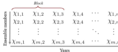
Figure 1.Schematic of the general reconstruction method using an

offline approach. Prior ensembles ofmstate vectors,χ, are assigned

to each of thenyears. To retain some temporal coherency, the rows

are composed of time-coherent blocks drawn from a climate model simulation (arbitrarily illustrated here as a 3-year block, or three consecutive annual states). The method updates prior ensembles for specific years corresponding to annual proxy data points, while for long-timescale proxies prior ensembles are computed by time av-eraging across the rows corresponding to the years of a proxy data point.

3. After all observations have been assimilated, the ensem-ble mean ofxbprovides the best estimate of the state for each analysis time.

We now discuss an illustrative implementation of this gen-eral algorithm that we employ for the experiments in this paper. Consider a paleoclimatic situation where the obser-vations are a collection of annual proxy data and also proxy data representing irregularly averaged climatic information. Let the prior ensembles be constructed, as we do in our ex-periments, by a random sample of annually averaged cli-mate states from a long clicli-mate simulation and initially as-signed to each year of a reconstruction (Fig. 1). Following the steps outlined above, proxies representing differently aver-aged time intervals can be assimilated by averaging over the prior ensembles for the time intervals defined by the proxy. For example, a proxy value representing information over the years 1700–1720 would update the prior ensembles averaged in time over that same interval. Annual proxies can simply be assimilated by updating the ensembles for each year of avail-able proxy data (Fig. 1). This approach proceeds by assim-ilating each proxy over its full time extent, and after every proxy is assimilated, one is left with an updated version of what one started with: a time sequence of ensemble state es-timates at annual resolution.

Moreover, in the offline case one may use hundreds to thou-sands of ensemble members from multiple models and sim-ulations, reducing the potential for model bias and sampling error. It is also advantageous to use an offline approach when the predictability time limit of the model is shorter than the timescale of the observations: for example, if observations are only available at annual resolution yet the model can-not skilfully forecast the climate state a year into the future, then no useful information is gained by cycling the model. Matsikaris et al. (2015) recently compared online and of-fline approaches to paleoclimate DA with a fully coupled Earth system model and found no improvement with the on-line method, suggesting that the model was unable to provide useful information at analysis times. Nevertheless, one way the approach outlined here can generalize to the online ap-proach is by cycling on the shortest timescale (e.g., annual or seasonal) and updating longer timescales at the end of the appropriate interval without cycling.

Also note that for the sake of simplicity in the illustra-tive example and throughout the paper, we are assuming that an irregular, long-timescale proxy is just an average of some climate variable over a given time interval. Real proxies are nearly always more complex than this and would necessitate a more sophisticated proxy system model (_H(xb) in Eqs. 1 and 2); however, the algorithm described above is general and covers the case when such models are available.

An important detail of the algorithm outlined above is that when updating the long-timescale states, the deviations from the time mean are not also updated. For most applications of this algorithm, we presume that there would be essen-tially two types of proxy timescales involved, annual and decadal timescales. Thus, we assume here that the decadal proxies would not inform annual climate variability. How-ever, there is no formal or practical obstacle that stops one from updating these deviations from the time mean (Huntley and Hakim, 2010). If, for example, one were working with proxies from two very similar timescales where there may be important shared covariance information, the deviations could also be updated by appending them to the mean states,

xb, and then proceeding with the algorithm.

One key point about the method outlined above is that if a reconstruction uses the offline approach together with multiple timescales, then a random sample of annually aver-aged climate states will not have meaningful multi-year av-erages. Temporal consistency of the priors will need to be ensured in order to have coherent long-timescale covariance relationships. One way to account for this is to draw priors in random blocks of consecutive years from the employed climate model simulation (see Fig. 1). The length of these blocks can be determined based on the needs of the spe-cific reconstruction problem (e.g., the length of the longest proxy timescale) and the length of available model simula-tions. If multiple long simulations are available (they need not be from the same model), different rows in Fig. 1 could be different model simulations and the block length could be

the length of the reconstruction; this option avoids any dis-continuities in time that result from small block lengths.

The DA technique of state space augmentation (as dis-cussed in, for example, Anderson, 2001) has long been used for handling arbitrary observation operators and can also be used for updating time-averaged quantities or parameter es-timation (e.g., Annan et al., 2005). Such an approach does have some important similarities to what we present here, particularly the ability to update time-averaged information. However, we are not aware of any paper that has worked out a multi-scale state augmentation approach for the paleocli-mate reconstruction problem. We think this could represent a viable approach, but it remains untested for paleoclimate reconstructions.

3 Experimental framework

3.1 Models and variable characterizations

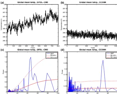
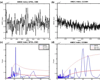
For the experiments presented here, we are interested in (1) how the reconstruction methodology proposed in Sect. 2 performs in both the atmosphere and ocean, (2) how the dif-fering timescales of the atmosphere and ocean may be lever-aged in the reconstruction process, and (3) how these results vary with two different models having quite different spectral characteristics in their coupled-climate systems. To this end we choose two long preindustrial control simulations (part of the Coupled Model Intercomparison Project Phase 5, avail-able for download at http://www.earthsystemgrid.org/), one from the climate model GFDL-CM3 (800 years in length) and the other from CCSM4 (1051 years in length). We also choose two illustrative reconstruction variables, global-mean 2 m air temperature and the Atlantic meridional overturn-ing circulation (AMOC). Figures 2 and 3 characterize the global-mean temperature and an AMOC index for each sim-ulation (defined here as the maximum value of the overturn-ing stream function in the North Atlantic between 25 and 70◦N and between depths of 500 and 2000 m), respectively. In these reconstructions the state vector,xb, only contains global latitude–longitude gridded values of 2 m air tempera-ture together with global-mean temperatempera-ture and the AMOC index as single-dimension appended state variables (rather than deriving them from the state vector itself)._H(xb) simply uses the surface temperature values of the state vector at the proxy locations. Note that even though these are only single-dimension variables, the DA framework proposed here can trivially reconstruct spatial variables as well (Steiger et al., 2014). From Figs. 2 and 3 we see that these two models dis-play different spectral characteristics for both global-mean temperature and the AMOC index.

ob-(a)

0 100 200 300 400 500 600 700 800 286

286.2 286.4 286.6 286.8 287 287.2 287.4 287.6 287.8

288 Global mean temp., GFDL−CM3

Temperature (K)

Years 0 200 400 600 800 1000

286 286.2 286.4 286.6 286.8 287 287.2 287.4 287.6 287.8

288 Global mean temp., CCSM4

Temperature (K)

Years

0 20 40 60 80 100

0 0.2 0.4 0.6 0.8 1 1.2 1.4

1.6 Global mean temp., GFDL−CM3

Period (years)

Power

GMT RN 95% RN mean

0 20 40 60 80 100

0 0.05 0.1 0.15 0.2 0.25 0.3

0.35 Global mean temp., CCSM4

Period (years)

Power

GMT RN 95% RN mean (b)

(c) (d)

Figure 2.Characterization of the global-mean 2 m air temperature variables used in this paper. Panels(a)and(b)show the global-mean

temperature time series for the preindustrial control simulations of GFDL-CM3 and CCSM4, respectively. Panels(c)and(d)show their

respective power spectra (GMT) with a best-fit red noise (RN) spectrum (computed as in Schneider and Neumaier, 2001) and an estimated 95 % confidence interval.

servations (Eq. 2). A simple assessment of this is shown in Fig. 4, which shows the correlation between the prior vari-ables and the surface temperature time series at the pseudo-proxy grid points for both climate simulations at a range of time averages. (Note that the correlation of two time series is simply the covariance normalized by the product of the standard deviations of the two time series.) Figure 4 indi-cates that there is increased covariance information (or more locations with higher correlations) between surface temper-ature and the prior variables at longer timescales. This in-formation is leveraged by the equations of DA to potentially improve the low-frequency components of the reconstructed variables. An important point about computing correlations at increasing time averages is that the number of degrees of freedom in the time series is also reduced, potentially spuri-ously inflating the correlations in Fig. 4. Accounting for these reduced degrees of freedom by performing a test of statisti-cal significance would not, however, be particularly germane: the DA equations do not “know” about 95 % confidence in-tervals, just the covariance information. If, after performing the reconstructions and computing several different skill met-rics, we see an increase in reconstruction skill, then we can

infer that the information was in fact useful for the recon-structions.

3.2 Pseudoproxy construction

be-(a) (b)

(c) (d)

0 100 200 300 400 500 600 700 800 2.2

2.4 2.6 2.8 3 3.2 3.4x 10

10 AMOC index, GFDL−CM3

AMOC (kg/s)

Years 0 200 400 600 800 1000

2.2 2.4 2.6 2.8 3 3.2 3.4x 10

10 AMOC index, CCSM4

AMOC (kg/s)

Years

0 20 40 60 80 100

0 0.5 1 1.5 2 2.5

3x 10

20 AMOC index, GFDL−CM3

Period (years)

Power

AMOC RN 95% RN mean

0 20 40 60 80 100

0 0.5 1 1.5 2 2.5 3

3.5x 10

19 AMOC index, CCSM4

Period (years)

Power

AMOC RN 95% RN mean

Figure 3.Characterization of the Atlantic meridional overturning circulation (AMOC) index variables used in this paper. Panels(a)and

(b)show the AMOC index time series (defined in the text) for the preindustrial control simulations of GFDL-CM3 and CCSM4, respectively.

Panels(c)and(d)show their respective power spectra with a best-fit red noise (RN) spectrum (computed as in Schneider and Neumaier,

2001) and an estimated 95 % confidence interval.

cause the purpose of the present work is primarily to illus-trate a new reconstruction method. The added noise is usu-ally assumed to be the same value for all proxy locations, with a common signal-to-noise ratio (SNR) being 0.5 (where SNR≡√var(X)/var(N), and whereX is a grid-point tem-perature series drawn from the true state, N is an additive noise series, and var is the variance.). Following recent work by Wang et al. (2014), we instead randomly draw SNR val-ues from a distribution characteristic of real proxy networks (Fig. 5b). This distribution is a shifted gamma distribution (shape parameter=1.667, scale parameter=0.18, shifted by 0.15) with a mean SNR of 0.45 and is modeled after Fig. 3 from Wang et al. (2014).

Also, in contrast to nearly all pseudoproxy experiments, we use pseudoproxies at two different timescales for each model. Importantly, we use the same SNR distribution for both timescales and add the noise to the time series after averaging. Within the DA framework, the additive error for each proxy is accounted for in the entries of the diagonal ma-trixR. The SNR equation above is related toRin that each of these entries is equal to var(N) for a given proxy. The process of adding the noise after averaging ensures that R

is statistically identical for each reconstruction. This process isolates the role of the covariance relationships in Eq. (2). By drawing from the same SNR distribution for all pseudo-proxy timescales we are also assuming that the distribution is an appropriate characterization of the error in long-timescale proxies; we assume this for simplicity and also because we are not aware of a systematic assessment of SNR values for low-resolution proxies as Wang et al. (2014) have done for annual-resolution proxies.

−0.4

−0.2

0 0.2 0.4 0.6 0.8 1

Time average (years)

Correlation (r)

Correlation of GMT with T2m, GFDL−CM3

1 5 10 15 20 25 35 50

−0.4

−0.2

0 0.2 0.4 0.6 0.8 1

Time average (years)

Correlation (r)

Correlation of GMT with T2m, CCSM4

1 5 10 15 20 25 35 50

−0.4

−0.2

0 0.2 0.4 0.6 0.8 1

Time average (years)

Correlation (r)

Correlation of AMOC index with T2m, GFDL−CM3

1 5 10 15 20 25 35 50

−0.4

−0.2

0 0.2 0.4 0.6 0.8 1

Time average (years)

Correlation (r)

Correlation of AMOC index with T2m, CCSM4

1 5 10 15 20 25 35 50

(a)

(b)

(c)

(d)

Figure 4.Panels(a)and(b)show the distribution of correlation values between the global-mean 2 m air temperature (GMT) and the 2 m air

surface temperatures (T2m) at the proxy locations for GFDL-CM3 and CCSM4 at a range of time averages. Panels(c)and(d)show similar

correlation distributions but for the correlation between the Atlantic meridional overturning circulation (AMOC) index and the 2 m air surface temperatures at the proxy locations. The correlations are computed for proxy grid points at a given time average, with the distribution of these correlations shown in gray dots and also summarized by box plots, where the blue boxes enclose the 25th and 75th percentiles and the

whiskers extend to±1.5 times this interquartile range.

(a)

(b)

0 0.5 1 1.5

0 0.5 1 1.5 2

2.5 SNR distribution (mean = 0.45)

SNR

Probability density

Pseudoproxy locations

Figure 5.(a)Pseudoproxy locations used in this study (n=274), drawn from the predominantly high-resolution (annual) proxy collection

of PAGES 2k Consortium (2013) and all the comparatively low-resolution (decadal to centennial) proxy locations in Shakun et al. (2012)

and Marcott et al. (2013).(b)The signal-to-noise ratio (SNR) distribution for the pseudoproxies, based on a real-world estimate of Wang

of real proxy climate reconstructions; using one simulation to reconstruct another can assess inter-model differences, but it is unclear how these results would relate to model–nature differences.

3.3 Pseudoproxy experiments

The primary results of this paper are presented in a series of 12 experiments using only atmospheric surface temperature pseudoproxies to reconstruct the global-mean temperature and AMOC index of the two climate model simulations dis-cussed previously. For each variable, and each model, three experiments are performed: (1) short (annual) pseudoproxies only, (2) long (5- or 20-year time averages) pseudoproxies only, and (3) both short and long time-averaged pseudoprox-ies. We have chosen the long timescale for the CCSM4 sim-ulation to be 20 years, and we note that an alternative choice of one to several decades gives similar results (not shown). The situation is more complex with the GFDL-CM3 sim-ulation because of the presence of an approximate 22-year periodic signal in the AMOC (Fig. 3a and c). A choice of 20 years for GFDL-CM3 would effectively undersample the AMOC variability, and so we have chosen a long timescale of 5 years for GFDL-CM3. Unfortunately, a long timescale of 5 years for CCSM4 shows little difference in the results over the annual timescale reconstructions (not shown), as would be suggested by the small difference in correlation (covari-ance) between 1 and 5 years (Fig. 4b, d).

Both the short-only and long-only reconstructions use 100 pseudoproxies randomly drawn from the network of 274 proxy locations shown in Fig. 5a. For the mixed-resolution reconstructions, 100 pseudoproxies are randomly drawn from the network for each timescale, giving a total of 200. This is an approximation of the real-world setting, where one usually has proxies at multiple timescales and would like to use all of them. Following the algorithm out-lined in Sect. 2, for the multi-scale reconstructions, we assim-ilate the long-timescale pseudoproxies first, followed by the annual timescale pseudoproxies; we also performed these re-constructions by swapping which timescale was assimilated first and found statistically identical results (not shown), as would be expected from the linearity of this approach. For these mixed-resolution reconstructions, we have also ensured that there is no overlap between locations associated with the two timescales.

We have reconstructed the first 400 years of each simula-tion while drawing the priors from the following 400 years of the simulations. Each year had a prior size of 1000 (e.g., from

Fig. 1, m=1000), while the blocks were randomly drawn

in 20-year continuous segments. This uniform block length was chosen because it was the longest timescale of the pseu-doproxies and because the pseupseu-doproxies were constructed over regular long intervals and thus discontinuities at block edges were not a concern (see Fig. 1 and the discussion in Sect. 2). Because the prior ensemble size was 1000, we did

not employ covariance localization, a common DA practice for controlling sampling error. Each of the 12 reconstruc-tions is repeated 100 times in a Monte Carlo fashion where new proxy networks and SNR values are randomly chosen each iteration; the new pseudoproxy networks are randomly drawn from the network shown in Fig. 5a and the SNR values are randomly drawn from the distribution shown in Fig. 5b. All the reconstruction figures show the mean of 100 of these Monte Carlo reconstruction iterations along with error bars indicating±2σ of the “grand ensemble” of analysis ensem-bles for all the Monte Carlo iterations (with an ensemble size of 1000 and 100 iterations, the grand ensemble has 1×105 members).

4 Reconstruction results

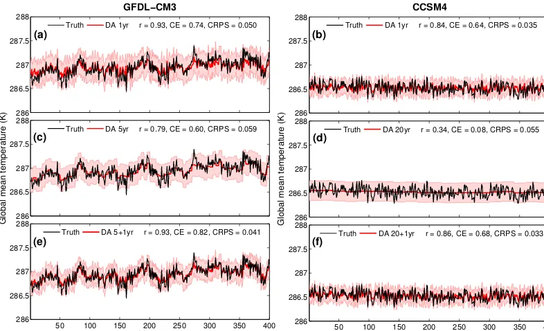
The reconstructions of global-mean temperature are shown in Fig. 6 along with their associated±2σ error estimates. In Fig. 6, panels (a) and (b) show the reconstructions with the annual pseudoproxies, (c) and (d) show the reconstructions with the long-timescale proxies, and (e) and (f) show the re-constructions for both timescales. Skill metrics, computed at annual resolution, are shown for each reconstruction: corre-lation (r), coefficient of efficiency (CE), and mean continu-ous ranked probability score (CRPS). The coefficient of ef-ficiency for a data series comparison of lengthN is defined as

CE=1−

PN

i=1(xi− ˆxi)2

PN

i=1(xi−x)2 ,

286 286.5 287 287.5

288 GFDL−CM3

Truth DA 1yr r = 0.93, CE = 0.74, CRPS = 0.050

286 286.5 287 287.5 288

Global mean temperature (K)

Truth DA 5yr r = 0.79, CE = 0.60, CRPS = 0.059

50 100 150 200 250 300 350 400

286 286.5 287 287.5 288

Years

Truth DA 5+1yr r = 0.93, CE = 0.82, CRPS = 0.041

286 286.5 287 287.5

288 CCSM4

Truth DA 1yr r = 0.84, CE = 0.64, CRPS = 0.035

286 286.5 287 287.5 288

Global mean temperature (K)

Truth DA 20yr r = 0.34, CE = 0.08, CRPS = 0.055

50 100 150 200 250 300 350 400

286 286.5 287 287.5 288

Years

Truth DA 20+1yr r = 0.86, CE = 0.68, CRPS = 0.033

(a)

(c)

(e)

(b)

(d)

(f)

Figure 6.Global-mean temperature reconstructions (mean of 100 Monte Carlo iterations, with error bars indicating±2σof the iterations and

analysis ensembles) for the three types of experiments discussed in the text and for each climate model simulation. Black lines indicate the true time series, while red lines indicate the reconstructed time series for only short-timescale (annual) pseudoproxies, only long timescale (5

or 20 years) pseudoproxies, and both long- and short-timescale pseudoproxies. Skill metrics of the reconstructions, correlation (r), coefficient

of efficiency (CE), and mean continuous ranked probability score (CRPS) are shown at the top of each subpanel.

(a) (b)

0 20 40 60 80 100

−0.05 0 0.05 0.1 0.15 0.2 0.25 0.3 0.35 0.4 0.45

Period (years)

Cross

power

spect

ral

densit

y

Global mean temp., GFDL−CM3

Truth

5+1 5 1

0 20 40 60 80 100

−0.01 0 0.01 0.02 0.03 0.04 0.05

Period (years)

Cross

power

spect

ral

densit

y

Global mean temp., CCSM4

Truth

20+1 20 1

Figure 7.Cross spectra of the reconstructed global-mean temperature time series with the true global-mean temperature time series, for

the reconstructions shown in Fig. 6. For reference, the dashed gray line indicates the cross spectra of the true time series with itself, or equivalently its own power spectrum.

Note that the long-timescale reconstructions shown in Fig. 6c and d have sharp edges at 5- (for GFDL-CM3) or 20-year (for CCSM4) intervals. This is due to the simplified experimental design we have employed where all the long-timescale pseudoproxies are averages over a given 5- or 20-year period. As discussed in Sect. 2, this experimental de-sign is only a single illustrative example of the general algo-rithm. The data from real proxies are not always apportioned into specific time frames but can be scattered irregularly in

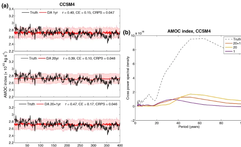
recon-Figure 8.AMOC index reconstructions (mean of 100 Monte Carlo iterations, with error bars indicating±2σ of the iterations and analysis ensembles) for the three types of experiments discussed in the text and for each climate model simulation. Black lines indicate the true time series, while red lines indicate the reconstructed time series for only short-timescale (annual) pseudoproxies, only long-timescale (5 or 20

years) pseudoproxies, and both long- and short-timescale pseudoproxies. Skill metrics of the reconstructions, correlation (r), coefficient of

efficiency (CE), and mean continuous ranked probability score (CRPS) are shown at the top of each subpanel.

structions many times and sampling from an age model for a given proxy.

One assessment of skill as a function of timescale is to compute the cross spectrum of the reconstructed time series with the true time series (Fig. 7). The cross spectra in this case reveal the relationship between the two time series as a function of frequency or period. As a point of reference, the dashed gray lines in this figure indicate the cross spectra of the true time series with itself, which is the same as its own power spectrum.1 Considering Fig. 7b we see that the annual-only reconstruction does a better job of matching the power at short periods than the 20-year-only reconstruction; however, the 20-year-only reconstruction performs better at longer periods. The mixed timescale reconstruction, 20+1, does better or just as well as the single-timescale reconstruc-tions at both short and long periods. This same general result holds for Fig. 7a, though it is more difficult to see because of the much larger power at longer periods in the GFDL-CM3 simulation.

Figure 8 shows three timescale reconstructions of the AMOC index for the two model simulations, similar to

1_{Following a common technique to reduce noise in the cross}

spectra, they are computed using Welch’s averaged periodogram method, which samples segments of the time series and averages the power spectra of these samples to arrive at the cross power spectral densities. As a result, the gray line spectra in Figs. 7 and 9 should not be expected to precisely match up with Figs. 2 and 3

val-ues between 0.6 and 0.4. Thus surface temperatures at the global proxy locations are relatively uninformative about the AMOC.

An additional result from Fig. 9 is the improved low-frequency components of the AMOC reconstructions when time-averaged surface temperature pseudoproxies are used. We argue that this result follows from the fact that the annual observations of atmospheric surface temperature are essen-tially noise to the slowly varying ocean. One may improve the information content relevant to the ocean by averaging over the atmospheric noise. This interpretation may also be seen in Fig. 4, where the correlation (covariance) informa-tion between the atmosphere and the ocean is particularly low at annual averages but improves at longer time averages (as also seen in Tardif et al., 2014). To further test this idea we performed mixed-resolution experiments in which the 100 pseudoproxies for each timescale were taken from the same locations. Therefore, here the long-timescale proxies are just the time-averaged versions of the annual proxies. We found essentially identical results with those shown in Figs. 6–9: all CRPS values were identical to three decimal places,rand CE were either identical to two decimal places or had changes of only±0.01, and there were no discernible differences in the cross spectra.

We note that all the cross spectra of the reconstructions shown in Figs. 7 and 9 show a decrease in power relative to the true state, though this need not always be the case. In ad-ditional experiments we performed using global ocean heat content, we found that this reconstructed variable tended to have more power than the true state and was thus higher than the respective dashed gray lines (not shown). Therefore the reduced power relative to the true state in Figs. 7 and 9 should not be interpreted as saying something general about the na-ture of DA-based reconstructions or the particular approach employed here.

As an approximation of a real reconstruction scenario, the experiments shown in Figs. 6 and 8 with two timescales use twice as many pseudoproxies as the single-timescale exper-iments (200 vs. 100). Therefore the improved skill might simply be a consequence of having more observation infor-mation. We tested this idea by repeating all the experiments shown here but instead increasing the number of observa-tions to 200 for each experiment: the single-timescale recon-structions used 200 randomly drawn pseudoproxies and the multi-scale reconstructions used 100 randomly drawn pseu-doproxies each for the two timescales (the same as in the previous multi-scale reconstructions). Figure 10 is a charac-teristic example of the results of these additional tests. Fig-ure 10a shows the reconstructions of the AMOC index with the CCSM4 model output and Fig. 10b shows the respective cross spectra. In (a), the skill is best for the multi-scale re-constructions and in (b) the cross spectra show the same gen-eral result of improved low-frequency power for the time-averaged pseudoproxies. However, the cross spectra for the 20+1 reconstruction are not always closest to the true

spec-trum, suggesting that the number of pseudoproxies does play a role in improving the spectrum of the reconstructions. In-deed, it should be the case that, as long as the proxies are unbiased, adding more of them will improve a DA-based re-construction.

5 Conclusions

This paper presents a data assimilation approach for paleo-climate reconstructions that can explicitly incorporate proxy data on arbitrary timescales. This approach generalizes previ-ous data assimilation techniques in the sense that many scales of both proxies and climate states can be included explicitly in a single reconstruction framework. The primary interest in such a reconstruction technique is that it allows for the inclusion of much more proxy data in climate reconstruc-tions. Given the spatially sparse and noisy nature of proxies, more information will tend to improve the quality of the re-constructions. Besides this benefit, using multi-scale proxy data may be particularly useful given the many inherent timescales of the climate system, such as the fast timescales of the atmosphere and the slow timescales of the ocean. We performed three types of realistic atmosphere–ocean pseudo-proxy reconstructions to assess the impact of using observa-tions at multiple timescales: (1) short (annual) pseudoproxies only, (2) long (∼decadal) pseudoproxies only, and (3) both short and long time-averaged pseudoproxies. We found for both global-mean temperature and an index of the AMOC that the reconstructions that incorporated proxies across both short and long timescales were more skillful than recon-structions that used short or long timescales alone (Figs. 6 and 8). This result holds even when the number of pseudo-proxies for the single-timescale reconstructions are doubled (Fig. 10a). Multi-scale reconstructions would be expected to perform better than single-scale reconstructions because they can include information at multiple timescales and because the prior can be better conditioned as it is used from one timescale to the next.

(a) (b)

0 20 40 60 80 100

−0.5 0 0.5 1 1.5 2 2.5 3 3.5 4 4.5x 10

19

Period (years)

Cross

power

spect

ral

densit

y

AMOC index, GFDL−CM3

Truth

5+1 5 1

0 20 40 60 80 100

−2 0 2 4 6 8 10x 10

18

Period (years)

Cross

power

spect

ral

densit

y

AMOC index, CCSM4

Truth

20+1 20 1

Figure 9.Cross spectra of the reconstructed AMOC index time series with the true AMOC index time series, for the reconstructions shown

in Fig. 8. For reference, the dashed gray line indicates the cross spectra of the true time series with itself, or equivalently its own power spectrum.

Figure 10.AMOC index reconstructions (mean of 100 Monte Carlo iterations, with error bars indicating±2σof the iterations and analysis

ensembles) and corresponding cross spectra similar to those shown in Figs. 8b, d, f and 9b but for the case where each experiment uses 200 pseudoproxies: the single-timescale reconstructions use 200 pseudoproxies each, while the multi-timescale reconstructions use 100 pseudoproxies for the short timescale and 100 pseudoproxies for the long timescale.

has a large covariance with the AMOC, the posterior will be more influenced by the observations. This result is not con-trolled by the noise added to the pseudoproxies because, as noted in Sect. 3.2, we ensured that Rfrom Eq. (2) remains fixed for both timescales.

These results indicate that DA-based atmosphere–ocean state estimates may be improved by including proxies and climate states from multiple timescales. The general results outlined above are consistent across the employed climate

such as salinity or indirect measures of ocean circulation may be better suited to reconstructing the AMOC.

6 Data availability

The GFDL-CM3 simulation is publicly available at http:// nomads.gfdl.noaa.gov/.

The CCSM4 simulation is publicly available at https:// www.earthsystemgrid.org/home.html.

Acknowledgements. We acknowledge the Program for Climate

Model Diagnosis and Intercomparison and the WCRP’s Working Group on Coupled Modeling for their roles in making available the CMIP5 data set. Support of the CMIP5 data set is provided by the US Department of Energy (DOE) Office of Science. This work was supported by the National Science Foundation (grant AGS-1304263) and the National Oceanic and Atmospheric Ad-ministration (grant NA14OAR4310176). We thank James Annan and three anonymous reviewers for their very helpful comments on previous versions of the paper.

Edited by: H. Goosse

References

Anderson, J. L.: An ensemble adjustment Kalman filter for data as-similation, Mon. Weather Rev., 129, 2884–2903, 2001.

Annan, J. D., Lunt, D. J., Hargreaves, J. C., and Valdes, P. J.: Pa-rameter estimation in an atmospheric GCM using the Ensem-ble Kalman Filter, Nonlin. Processes Geophys., 12, 363–371, doi:10.5194/npg-12-363-2005, 2005.

Bradley, R. S.: Paleoclimatology, Academic Press, Oxford, UK, 3rd edn., 2014.

Carro-Calvo, L., Salcedo-Sanz, S., and Luterbacher, J.: Neural com-putation in paleoclimatology: General methodology and a case study, Neurocomputing, 113, 262–268, 2013.

Dirren, S. and Hakim, G. J.: Toward the assimilation of time-averaged observations, Geophys. Res. Lett., 32, 4, doi:10.1029/2004GL021444, 2005.

Evans, M. N., Tolwinski-Ward, S., Thompson, D., and Anchukaitis, K. J.: Applications of proxy system modeling in high resolution paleoclimatology, Quaternary Sci. Rev., 76, 16–28, 2013. Gneiting, T. and Raftery, A. E.: Strictly proper scoring rules,

pre-diction, and estimation, Journal of the American Statistical As-sociation, 102, 359–378, 2007.

Goosse, H., Crespin, E., Dubinkina, S., Loutre, M.-F., Mann, M. E., Renssen, H., Sallaz-Damaz, Y., and Shindell, D.: The role of forcing and internal dynamics in explaining the “Medieval Cli-mate Anomaly”, Clim. Dynam., 39, 2847–2866, 2012.

Guiot, J. and Corona, C.: Growing season temperatures in Europe and climate forcings over the past 1400 years, PloS one, 5, e9972, doi:10.1371/journal.pone.0009972, 2010.

Hanhijärvi, S., Tingley, M., and Korhola, A.: Pairwise compar-isons to reconstruct mean temperature in the Arctic Atlantic Re-gion over the last 2,000 years, Clim. Dynam., 41, 2039–2060, doi:10.1007/s00382-013-1701-4, 2013.

Houtekamer, P. L. and Mitchell, H. L.: A sequential ensemble Kalman filter for atmospheric data assimilation, Mon. Weather Rev., 129, 123–137, 2001.

Huntley, H. S. and Hakim, G. J.: Assimilation of time-averaged ob-servations in a quasi-geostrophic atmospheric jet model, Clim. Dynam., 35, 995–1009, doi:10.1007/s00382-009-0714-5, 2010. Kalnay, E.: Atmospheric modeling, data assimilation and

pre-dictability, Cambridge, Cambridge, UK, 2003.

Kurahashi-Nakamura, T., Losch, M., and Paul, A.: Can sparse proxy data constrain the strength of the Atlantic meridional overturning circulation?, Geosci. Model Dev., 7, 419–432, doi:10.5194/gmd-7-419-2014, 2014.

Li, B., Nychka, D. W., and Ammann, C. M.: The value of multi-proxy reconstruction of past climate, J. Am. Stat. Assoc., 105, 883–895, 2010.

Mann, M. E., Rutherford, S., Wahl, E., and Ammann, C.: Testing the fidelity of methods used in proxy-based reconstructions of past climate, J. Climate, 18, 4097–4107, 2005.

Mann, M. E., Zhang, Z., Hughes, M. K., Bradley, R. S., Miller, S. K., Rutherford, S., and Ni, F.: Proxy-based reconstructions of hemispheric and global surface temperature variations over the past two millennia, P. Natl. Acad. Sci. USA, 105, 13252–13257, doi:10.1073/pnas.0805721105, 2008.

Marcott, S. A., Shakun, J. D., Clark, P. U., and Mix, A. C.: A Recon-struction of Regional and Global Temperature for the Past 11,300 Years, Science, 339, 1198–1201, doi:10.1126/science.1228026, 2013.

Mathiot, P., Goosse, H., Crosta, X., Stenni, B., Braida, M., Renssen, H., Van Meerbeeck, C. J., Masson-Delmotte, V., Mairesse, A., and Dubinkina, S.: Using data assimilation to investigate the causes of Southern Hemisphere high latitude cooling from 10 to 8 ka BP, Clim. Past, 9, 887–901, doi:10.5194/cp-9-887-2013, 2013.

Matsikaris, A., Widmann, M., and Jungclaus, J.: On-line and off-line data assimilation in palaeoclimatology: a case study, Clim. Past, 11, 81–93, doi:10.5194/cp-11-81-2015, 2015.

PAGES 2k Consortium: Continental-scale temperature variabil-ity during the past two millennia, Nat. Geosci., 6, 339–346, doi:10.1038/ngeo1797, 2013.

Schneider, T. and Neumaier, A.: Algorithm 808: ARfit – A Mat-lab package for the estimation of parameters and eigenmodes of multivariate autoregressive models, ACM Transactions on Math-ematical Software (TOMS), 27, 58–65, 2001.

Shakun, J. D., Clark, P. U., He, F., Marcott, S. A., Mix, A. C., Liu, Z., Otto-Bliesner, B., Schmittner, A., and Bard, E.: Global warm-ing preceded by increaswarm-ing carbon dioxide concentrations durwarm-ing the last deglaciation, Nature, 484, 49–54, 2012.

Smerdon, J. E.: Climate models as a test bed for climate reconstruc-tion methods: pseudoproxy experiments, WIREs Clim. Change, 3, 63–77, doi:10.1002/wcc.149, 2012.

Steiger, N. J., Hakim, G. J., Steig, E. J., Battisti, D. S., and Roe, G. H.: Assimilation of time-averaged pseudoproxies for climate reconstruction, J. Climate, 27, 426–441, doi:10.1175/JCLI-D-12-00693.1, 2014.

Wang, J., Emile-Geay, J., Guillot, D., Smerdon, J. E., and Rajarat-nam, B.: Evaluating climate field reconstruction techniques using improved emulations of real-world conditions, Clim. Past, 10, 1– 19, doi:10.5194/cp-10-1-2014, 2014.