Scale-Invariant Feature Transform Algorithm with Fast Approximate Nearest Neighbor Ekhlas Khalaf Gbash | Suha Mohammed Saleh

Accepted 21/6/2017

This work is licensed under a Creative Commons Attribution 4.0 International License.

Abstract:

There is a great deal of systems dealing with image processing that are being used and developed on a daily basis. Those systems need the deployment of some basic operations such as detecting the Regions of Interest and matching those regions, in addition to the description of their properties. Those operations play a significant role in decision making which is necessary for the next operations depending on the assigned task.

In order to accomplish those tasks, various algorithms have been introduced throughout years. One of the most popular algorithms is the Scale Invariant Feature Transform (SIFT). The efficiency of this algorithm is its performance in the process of detection and property description, and that is due to the fact that it operates on a big number of key-points, the only drawback it has is that it is rather time consuming. In the suggested approach, the system deploys SIFT to perform its basic tasks of matching and description is focused on minimizing the number of key-points which is performed via applying Fast Approximate Nearest Neighbor algorithm, which will reduce the redundancy of matching leading to speeding up the process.

The proposed application has been evaluated in terms of two criteria which are time and accuracy, and has accomplished a percentage of accuracy of up to 100%, in addition to speeding up the processes of matching and description.

Keyword: Invariant Features, Object Recognition, Scale Invariance, Image Matching, Sift Algorithm.

Introduction:

Extracting and matching properties are one of the most common issues facing the computer vision field, like object identification or structure from movement. Property detection and image matching are considered as two significant problems in computer vision, graphics, photogrammetric and the majority of images applications every day. Their application keeps growing in different areas. [1].

characterization of local image properties. It offers the ability of precise object recognition with low possibility of mismatching and is easy to be matched against a large data-base of local properties. The representation of the image properties has a great effect on the results of an object identification system [2].

Regions of Interest are defined as those contain user defined items of significance, and a sufficient algorithm is produced to detect such areas.

In this study, a suggested approach that depends on the algorithm of SIFT in finding the Region of Interest in image. Moreover, in the Suggested approach of this algorithm has been developed for the sake of giving better results in terms of precision and speed measures [3].

1. SIFT (Scale-invariant Feature Transform):

SIFT was introduced by David Lowe. As it is clear from its name, this algorithm’s reason is transforming the image-data into SIFT coordinates related to the local properties .Lowe benefitted from the properties for the sake of executing matching procedures between distinct images of the same scenes or objects.

The extracted features are invariant to image rotating and scaling, and they offer very strong matching over a basic domain of affine distortion, three-dimensional viewpoint change, adding noise and changing in lightness. In addition, the properties are very distinctive, which mean that one property might be properly matched

with high degree of probability against a large property data-base[4].

For matching a new image, each property extracted from the new image is compared separately to the properties that are stored in the data-base.

1.1 Feature Extraction

A set of local properties of an image is extracted from every image. Each of those properties includes a registry of: 1.Position, or pixel location (x, y), of the image.

2.Scale, characterized by the standard deviation σ.

3.Orientation, the dominating direction of the image structure in the neighborhood.

4.Detailing of the image’s local structure, characterized according to gradient histograms.[4]

The main steps of computation

implemented for generating the group of properties are:

Fig. 1: Construction of difference-of-Gaussian images [5]

The DOG pyramid D(x,y, σ) is calculated from the difference of every2neighboring images in Gaussian pyramid Fig 2. The local extrema (maxima or minima) of DOG function are found via the comparison of every one of the pixels with its 26 adjacent pixels in the scale-space (8 neighbors in the same scale, 9 corresponding neighbors in the scale above and 9 neighbors in the scale below). The searching for extrema eliminates the first and the last image in every one of the octaves due to the fact that they don’t have a scale above and a scale below [5].

• Localizing the key-points- the detected local extrema are efficient nominees for key-points. On the other hand, they should be precisely localized via fitting a three dimensional quadratic function to the scale-space local sampling point. The quadratic function is calculated with the use of a 2nd order

Taylor expansion that has the origin at the sample point. Afterwards, local

Fig. 2: Pixel comparisons to detect maxima and minima of difference-of-Gaussian image [5]

extrema with low contrast and such that correspond to edges are gotten rid of due to the fact that they’re of high sensitivity to noise [6].

• Assigning the orientation–as soon as

gradients [7]. For every one of the pixels of the area surrounding the property position the gradient magnitude and orientation are calculated according to:

M(X,Y)=√

(𝐿(𝑋 + 1, 𝑌, 𝜕))𝑥𝑥2 ₊

(𝐿(𝑋, 𝑌 + 1, 𝜕) − 𝐿(𝑋, 𝑌 − 1, 𝜕) ) 𝑥^𝑥2

2

(EQ 1) Ө(X,Y)=arctan((l(x.y+1, 𝜕

)-l(x,y-1, 𝜕))/(𝑙(𝑥 = 1, 𝑦, 𝜕) − 𝑙(𝑥 − 1, 𝑦, 𝜕))) (Eq 2) The gradient magnitudes are weighted by a Gaussian window whose size is dependent on the property octave. The weighted gradient magnitudes are used for establishing a direction histogram having 36 bins that cover the 360◦ direction range. The highest orientation histogram peak and peaks with amplitudes higher than 80% of the highest peak are used for the sake of creating a key-point with this direction. Thus, there will be more than one

key-point generated at the same position but with varying directions [8].

• Descriptor of the Keypoint- the area that is surrounding a key-point is split into 4X4 boxes Fig 3. The gradient magnitudes and directions in every one of the boxes are calculated and weighted by suitable Gaussian window, and the coordinate of every one of the pixels and its gradient direction under go rotation according to the key-points direction. Afterwards, for every one of the boxes an 8 bins orientation histogram is determined[8]. From the 16 obtained orientation histograms, a 128D vector (SIFT-descriptor) is constructed. This descriptor is independent of the orientation, due to the fact that it is computed according to the main direction. Lastly, for the sake of achieving the independence from variation in illumination, the descriptor is normalized to unit length [9].

Fig. 3: Computation of the keypoint descriptor [10]

2. proposed system structure:

Mainly the proposed system consists of four main steps (Figure4):

 Preprocessing.  RANSAC.  SIFT.

 Fast approximate nearest neighbor.

Fig.4: proposed system steps

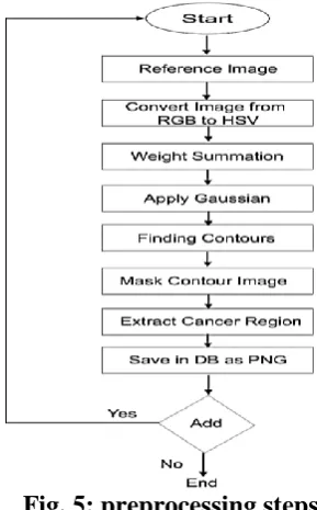
2.1 Preprocessing step:

It is known that most of the image processing operations don’t begin unless a preprocessing operation is performed first. Its goal is enhancement of the target image for the sake of getting better results in further processing. The preprocessing operation that is performed on the image is shown in Figure 5:

Preprocessing

RANSAC

SIFT

Fig. 5: preprocessing steps

Mainly the preprocessing consists of the following steps:

 Converting Input Image into HSV form

The result of this operation is depicted in the figures below:

Fig. 6: the Original Acquired Image

Fig. 7: Converting Images from RGB to HSV Color Format

 Thresholding Process

In this step, the image that was resulted from the previous step is an image in HSV form. This step thresholds that image for every area that is not red colored which is done by choosing a single value from the resulted image which is the hue, rather than having to identify the desired area from three values (i.e. RGB) where the hue is of values that lie between 0 and 180, while the values of the saturation and the intensity have the range between 0 and 255.

The results of this stage are depicted in the images below:

Fig. 9: The Lower Range Values of the Images in Figure 7.

 Applying the Summation

This step is done to combine the two images that resulted from the thresholding step to produce one image that will be further processes to complete the rest of the operation. Figure 10 shows the results of this stage:

Fig. 10: the Results of Applying Summation on the Images Resulted from the Previous Step

 Gaussian Blurring

This operation is used in order to smooth the image and eliminate the noise and some unwanted details that may degrade the quality of the subsequent processing therefore this step works on improving the resulted image. Figure 11 shows the results of this stage:

Fig. 11: the Result of Applying Gaussian Blurring Filter

 Applying Mask for Contour Detection

 Extracting and Storing the Region of the Interest

2.2 RANSAC:

This algorithm is applied to bounder the keypoints (final keypoints) obtained from the SIFT and then from SIFT with approximate, the algorithm is worked by choosing points from specified image and generate candidate structure of the wanted property, In our system the points selected are the keypoints and minimum three points needed to define specific property (sick part), This algorithm can be applied to (original SIFT, SIFT with approximate or any image) .

2.3 SIFT:The Original SIFT Are Applied To the Image:

Fig. 12: DOG discrete extrema

 The Filtration of Keypoints that is considered Unstable is done by thresholding, as shown in figure 13.

Fig. 13:DOG after thresholding

 The candidate keypoint will be minimized after applying the refinement 3D extrema Figure 14.

Fig. 14: candidates after refinement 3D extrema

 The keypoints lying on edges are discarded to minimize the unusual information obtained by the algorithm and the results obtained are in Figure 15.

Fig. 15:Candidates After Discarding Points Lying On Edges

Fig. 16:After Applying SIFT Stages

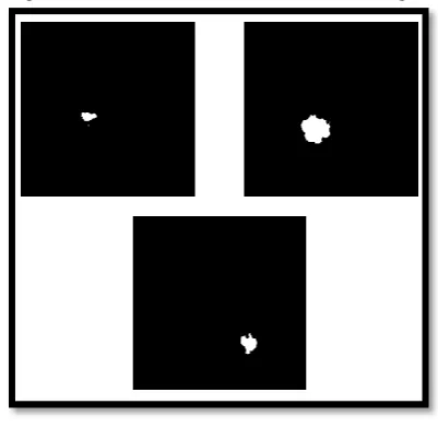
Our system recognized the parts that is useful for lung cancer before applying the original SIFT and the SIFT with approximate, Figure 17 shows the region of interest that cut out the sick part by applying many algorithms, the chosen image will be converted to HVC and then a threshold is applied to detect the possible sick area (sick are is colored red) the sick part is bounded by applying RANSAC algorithm after the preprocessing step.

Fig. 17:Region of Interest In Image 1

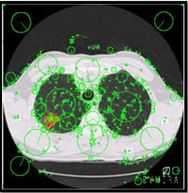
By applying the SIFT algorithm to region of interest part the number of keypoints obtained will be specifically to the sick part, as shown in Figure 18.

Fig. 18:The Sick Part Recognition

2.4SIFT key points result with Fast approximate nearest neighbor:

Computing the distance from the query to each of the single points in the SIFT resulted key points and return the nearest one will lead to discard some points that are considered far form group of key points; Figure 19 shows image1 after applying the approximate .

points in less time, while obtaining the

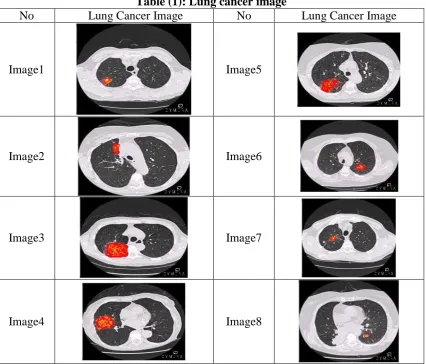
Table (1): Lung cancer image

No Lung Cancer Image No Lung Cancer Image

Image1 Image5

Image2 Image6

Image3 Image7

Table (2): a comparison between the original SIFT and the proposed system in terms of the number of keypoints

Recognition lung area Keypoint for matching lung area

No _Proposed

Method Original SIFT Proposed Method Original SIFT True True 7 9 Image1 True True 8 10 Image2 True True 50 55 Image3 True True 52 58 Image4 True True 28 46 Image5 True True 11 15 Image6 True True 17 18 Image7 True True 12 13 Image8 100% 100% 158 224 Total

Table (3) the comparison between both systems in terms of time efficiency

Matching Time No Proposed Method Original SIFT 0.164 0.428 Image1 0.365 0.394 Image2 0.365 0.501 Image3 0.726 0.828 Image4 0.9 0.982 Image5 0.864 0.939 Image6 1.033 1.219 Image7 1.202 1.309 Image8 5.619 6.6 Total

Conclusion

:

In

this

research

we

submitted the following points:

1-The proposed system can minimize the number of keypointsan determine only the important keypoints which allow the system to make the detection, description and matching of the ROI(region of interest) in very quickly way.

2- The main problem of the SIFT algorithm is that it required time to provide the detection, description and matching of the ROI. So to avoid this problem, fast approximation matching algorithm is used.

In future work, SURF(Speeded-Up Robust Features algorithm) can be used with fast approximate nearest neighbor in order to reduce the number of features and time .

References

:

[1]Vinukonda, P. 2011. A Study of the Scale-Invariant Feature Transform on a Parallel Pipeline. Proc. 9th IEEE International Conference on Computer Vision,. pp: 5-14.

[2]Ouyang, W. 2010. Based Descriptors for Object Recognition.V o l u me 6, Issue 3.211-144.

[3]Kim, D. and Hwang E. 2012. Local feature base multi-object recognition scheme for surveillance. Engineering Applications of Artificial Intelligence, 25 (7),pp: 1373–1380. [4] Morteza, Z. and Saeideh E. 2011.

Farsi/Arabic Optical Font Recognition Using SIFT Features. Procedia Computer Science 3 1055– 1059.

Di. and Cham, L. 2012.Performance

ليوحت ةيمزراوخ

راج برقلا عيرسلا بيرقتلا عم سايقمب ةرثاتملا ريغ صئاصخلا

شابك فلخ صلاخا

حلاص دمحم اهس

نكتلا ةعماجلا،تابساحلا مولع مسق و

،ايجول ،دادغب قارعلا .

:ةصلاخلا

نم هذه.صاوخلا هذه فيصوت ىلا ةفاضلااب،قطانملا هذه ةقباطمو ةمهملا قطانملا فاشتكاك ةيساسلاا تايلمعلا تامهملا ىلع دامتعلااب ةقحلالا تايلمعلل يرورض نوكي يذلارارقلا ذاختا يف مهم رود تبعل تايلمعلا

.ةصصخملا لاخ تمدق تايمزراوخلا نم ديدعلا،ةصصخملا تايلمعلا قيقحت لجا نم رهشا نم ةدحاو.ةيضاملا تاونسلا ل

(يه تايمزراوخلا تايلمع يف ةءوفك ةيمزراوخلا هذه .)سايقمب ةرثاتملا ريغ صئاصخلا ليوحت ةيمزراوخ

ةجلاعملا ةيلمعل ليوط تقو قارغتسا ىلا ىدا ةيحاتفملا طاقنلا ةرثك نكل ةيحاتفملا طاقنلل فيصوتلاو فاشتكلاا مزراوخلا هذه بويع نم ربتعي يذلا .ةي

ىلع زيكرتلا متو فيصوتلاو فشكلا يف ةيساسلاا ماهملا ةيداتل ةيمراوخلا فظو ماظنلا ، ةحرتقملا ةقيرطلا يف يتلاو ةرركتملا طاقنلا نم للقت يتلا راج برقالا عيرسلا بيرقتلا ةيمزراوخ مادختساب ةيحاتفملا طاقنلا ددع ليلقت .ةجلاعملا ةيلمع عيرست ىلا يدوت اظنلا مييقت مت ةقد ةبسن قيقحت متو ، ةقدلاو تقولا امه نييرايعم ىلع دامتعلااب حرتقملا م

100 ىلا ةفاضلااب %

.ةجلاعملا ةيلمع عيرست

:ةيحاتفملا تاملكلا