Monitoring Jovian Orbital Resonances of a Spacecraft: Classical and Relativistic Effects

(1)

universe

Article

Monitoring Jovian Orbital Resonances of a Spacecraft:

Classical and Relativistic Effects

Luis Acedo

Department of Mathematics, Centro Universitario de Plasencia, Avda. Virgen del Puerto, 2, University of Extremadura, 10600 Plasencia, Spain; acedo@unex.es; Tel.: +34-927-427000 (ext. 52306)

Received: 28 October 2019; Accepted: 28 November 2019; Published: 3 December 2019

Abstract:Orbital resonances continue to be one of the most difficult problems in celestial mechanics. They have been studied in connection with the so-called Kirkwood gaps in the asteroid belt for many years. On the other hand, resonant trans-Neptunian objects are also an active area of research in Solar System dynamics, as are the recently discovered resonances in extrasolar planetary systems. A careful monitoring of the trajectories of these objects is hindered by the small size of asteroids or the large distances of the trans-Neptunian bodies. In this paper, we propose a mission concept, called CHRONOS (after the greek god of time), in which a spacecraft could be sent to with the initial condition of resonance with Jupiter in order to study the future evolution of its trajectory. We show that radio monitoring of these trajectories could allow for a better understanding of the initial stages of the evolution of resonant trajectories and the associated relativistic effects.

Keywords:orbital resonance; general relativity; celestial mechanics perturbations; radar ranging

1. Introduction

In recent years, the interest in spacecraft missions to study orbital dynamics in general relativity and other effects has soared, in part due to the discovery of some possible astrometric anomalies that challenge our current understanding of gravity [1,2]. In particular, we have the anomalous secular increase of the lunar eccentricity, which has not been completely explained within the context of the models of tidal interactions in the Moon–Earth system [3,4]. The flyby anomaly has also generated a wide interest [5], as has the Pioneer anomaly [6], although the latter can now be explained in terms of the anisotropic thermal emission of the heat generated by the radioisotope thermoelectric generators of the spacecraft [7,8]. The solution of the problems posed by these anomalies could be found in some of the proposed, or future, extensions of the theory of general relativity. Corda has provided a method that might be used to elucidate the correct framework for general relativity [9]. The idea is to check the angle- and frequency-dependent response functions of gravitational wave interferometers. This could be a reality in the future if the sensitivity of gravitational wave detectors is adequately improved.

Studies of planetary and asteroid orbits started a long time ago. In a paper published in 1866, the American astronomer D. Kirkwood performed the first statistics of the orbits of many asteroids in the asteroid belt located between Mars and Jupiter [10]. In this study, Kirkwood noticed that, at some particular distances from the Sun, there are marked gaps or depletions in the numbers of asteroids. He explained this fact in terms of the ratio among the periods of an asteroid in that gap and the orbital period of Jupiter around the Sun. For the ratios 4:1, 3:1, 5:2, 7:3, and 2:1 it seems that asteroids, perhaps occupying this position in an earlier time, were ejected by periodic perturbations with Jupiter. This explanation was extended to the Cassini division in Saturn’s rings, now attributed to a 2:1 destabilizing resonance with the moon Mimas [11].

In the forties and early fifties of the past century, the idea of a region beyond the orbit of Neptune, in which the primordial planetary nebulas had condensed into a myriad of small bodies, took form

(2)

by the suggestions of Edgeworth and Kuiper [12]. The discovery of many objects between 30 and 50 AU from the Sun give rise to the modern concept of a trans-Neptunian belt, which, on the other hand, does not correspond exactly with the initial formulation of Edgeworth-Kuiper. In this belt, we have some stabilizing resonance ratios with Neptune. In particular, the 2:3 resonance is occupied by Pluto, the plutino family, and the 1:2 resonance by the twotinos [13].

The recent discovery of many extrasolar systems have also become a fertile ground for the study of resonances. In some of these systems, resonant behavior has been unraveled. For example, the system around the red dwarf Gliese 876 contains three exoplanets, named “e”, “b”, and “c”, which are in a chained 4:2:1 resonance [14]. A four-planet resonance has also been found in the Kepler-223 system. The period ratio is, in this case, 3:4:6:8. Planetary migration is the more likely cause of this arrangement [15].

The commensurability 2:1 with Jupiter has been particularly difficult to analyze. In the classical context of the planar, circular-restricted three-body problem, the corresponding resonance seems to be stable. However, a depletion of objects was clearly observed since the analysis of Kirkwood. This puzzle has been attacked by many authors. Lemaitre and Henrard disclosed a source of chaos in the low-eccentricity regime of this resonance [16]. Secular resonances inside the 2:1 commensurability were later discovered by Morbidelli and Moons [17]. It was found that low eccentricity orbits can evolve into high eccentricity ones. Simulations for test particles with eccentricitiese<0.355 and inclinations ι<1.5◦showed median lifetimes of 80 million years [18]. This way, a destabilizing mechanism for previously proposed islands of stability was disclosed. There are still certain quasi-regular islands of stability populated by remnants of the Themis family [19].

The presence of chaos in the Solar System is not restricted to the most conspicuous resonances. According to the discoveries of Laskar, Quinn, Tremaine, and others [20,21], the whole Solar System exhibits chaotic dynamics with a typical Lyapunov exponent of 1/5 Myr−1. Orbital integration to simulate the evolution of the whole system in the next five billion years showed that even planetary collisions or ejections cannot be discarded before the end of the life cycle of the Sun [22]. These large-scale simulations cannot be carried out with standard numerical methods but they require, instead, symplectic integrators [23]. Symplectic integrators have many advantages in dynamic astronomy in comparison with the Runge–Kutta or the Adams–Bashforth–Moulton predictor-corrector methods [24]. In particular, numerical solutions are area-preserving, discretization errors of the energy integral have no secular terms, and the integration of highly eccentric orbits is possible without step-size changes. Other merits of some special methods can be the exact conservation of the total angular momentum or time reversibility of the numerical solution [25]. These properties have proven essential in obtaining sensible solutions for the integrations in a very large number of orbits [22]. On the other hand, the ephemerides developed for spacecraft navigation are usually based upon classical methods since the late sixties. For example, Lieske reported in 1967, on one of the earliest versions of the ephemeris for the period 1800–2000 that was based upon the Adams-Störmer method [26]. Similar methods, but improved, have been used in subsequent versions [27].

Another important issue concerning highly-accurate orbital integration over prolonged periods of time is the incorporation of relativistic corrections. This is a challenging problem that has pervaded the history of general relativity since its 1915 formulation. In general relativity, particles move along the geodesics of a curved space-time manifold generated by the other bodies in its neighborhood. For an overview of the recent status of general relativity and some future perspectives, see, for example, the editorial by Iorio [28], and the reviews of Debono and Smoot [29] or Vishwakarma [30].

(3)

was proposed by Einstein himself in collaboration with Infeld and Hoffmann in 1938 [33]. This EIH approach can be applied to a system of point-like particles under their mutual gravitational interactions. This is a first-order post-Newtonian approximation. Higher-order approximations are possible, and even those taking into account a reaction to the gravitational radiation [34], but, for the purpose of studying the Solar System dynamics, the EIH is considered sufficiently accurate [35]. The equations of motion in general relativity include "cross-terms" in the post-Newtonian approximation involving the interaction with the Sun and other planets as well. By taking into account this effect and the gravitomagnetism of the moving planets, Will recently deduced a new contribution to the anomalous perihelion advance of Mercury [36].

In this paper we describe a study on the orbital dynamics of a spacecraft located at an initially circular orbit around the Sun within a distance allowing for resonance with Jupiter. To perform the integrations, we compare the traditional, explicit numerical methods with the symplectic partitioned Runge–Kutta method. For human timescales, both methods yield equivalent results, and consequently, for the time span of the spacecraft mission a convenient approach may ignore the subtleties of the most sophisticated integration methods. As the Lyapunov exponent for Solar System dynamics is known to be in the range of 1/5 Myr−1[22], no signs of classical chaos were expected to emerge from a study restricted to a period of decades concerned with the planetary orbits. Nevertheless, some indication of irregular, non-periodic behavior in the contribution of the relativistic corrections may be disclosed in this period of time, and in the case of resonant orbits, chaotic motion in certain configurations may arise. In connection with the mission proposal in this paper, we should notice that Iorio has also proposed a Jovian probe to test the post-Newtonian gravitomagnetic spin octupole of Jupiter [37]. However, our focus is on the classical resonant trajectories and their modification by general relativistic corrections to the equations of motion instead of the gravity field of Jupiter in itself.

The paper is organized as follows: In Section2, we propose a simple geometric model for the study of perturbations of a major planet on a spacecraft orbiting around the Sun. In this section, we consider the classical Newtonian effects and compare several methods of integration. Section3is devoted to the analysis of the Einstein–Infeld–Hoffmann post-Newtonian corrections for the three-body system composed of the Sun, Jupiter, and the spacecraft. With the integration of this system, we show that the detection of the relativistic corrections is within reach of present radio technology and they will be manifested after a few years of the start of the mission. The paper ends with a discussion on the interest of a mission designed to study celestial mechanics resonances.

2. Modelling Jovian Resonances: The Newtonian Approach

In this section we consider a simplified model for the orbital resonance of the spacecraft with Jupiter in the context of the restricted, 3-body problem of celestial mechanics.

The initial conditions for the spacecraft and Jupiter are plotted in Figure1.

If we denote byR0the average distance of Jupiter to the Sun andT0its orbital period, the Cartesian coordinates of this planet in the orbital plane would be given by:

Rx(t) = R0 cos

2πt T0

+φ

,

Ry(t) = R0 sin

2πt T0

+φ

.

(1)

Hereφis the initial angle of the position vector of Jupiter with respect to the position vector of the spacecraft. It is convenient to use normalized quantities by usingR0as unit of distance and τ=T0/(2π) =R3/2₀ /√µas unit of time. For Jupiter, we haveR0=5.204 AU andT0=11.862 years. The mass constant of the Sun isµ = 132, 712, 440, 018 km3/s2and we can also define the unit of

velocity asp

(4)

canonical variablesqx,qy,px, andpyfor the position and momentum, the Hamiltonian per unit mass is then given by:

H = p 2 x 2 +

p2y 2 −

1

q q2

x+q2y

− q κ

(qx−Rx(t))2+ (qy−Ry(t))2 ,

(2)

whereκ=µJ/µis the mass ratio of Jupiter and the Sun (κ=0.000954601) and all the quantities are scaled,Rx(t)→Rx(t)/R0, etc.

R

r

Figure 1.Ideal circular orbits for Jupiter and the spacecraft in the 2:1 resonant configuration. The position vector of Jupiter with respect to the Sun is denoted byRandrfor the spacecraft. Initially, there is an angular difference ofφradians in their orbital positions.

The semi-major axis of the spacecraft osculating orbit at the initial condition is given bya= f2/3 (in units of R0), where f is the ratio of the orbital period of the spacecraft with respect to Jupiter; i.e.,f =1/2 for the resonance 2:1. According to Figure1we take the initial conditions for the spacecraft aspx(0) =0,py(0) =√1/a,qx(0) =a, andqy(0) =0. A symplectic partitioned Runge–Kutta method of difference order 4 was used for integration, with an initial step size,∆t = 2π/100. Integration was carried out for a period of 20T0, corresponding to 237 years. The results for the distance of the spacecraft to the Sun in the resonance 1:1 (withφ = ±π/8) are plotted in Figure2. We observe a complicated, but periodic, pattern with no hint of chaos in this approximation. Anyway, it should be noticed that the large perturbations induced by Jupiter expel the spacecraft from the circular orbit at distances to the Sun ten per cent larger or smaller than the original distance.

Although the initial osculating orbit is assumed to be circular, the perturbations transform it into an elliptical one with a variable eccentricity. Therefore, it is also interesting to analyze the evolution of other orbital parameters with time. In Figure3, we have plotted the argument of the perihelion as a function of scaled time. We see that, in this particular configuration, there is a retrograde motion of the perihelion in the range of several degrees per century.

(5)

0 5 10 15 20 0.90

0.95 1.00 1.05 1.10

r

(

t

)

(

R

0

)

t (T

0

)

Figure 2.Distance of the spacecraft to the Sun in the resonance 2:1 with Jupiter. The initial phase is

φ=π/8 (solid line) andφ=−π/8 (dotted line). Units of distance and time are scaled.

0 5 10 15 20 25 30 35

0 20 40 60 80 100

(

D

e

g

r

e

s

)

t (T

0

)

Figure 3.Argument of the perihelion for a spacecraft in the resonance the resonance 1:1 with Jupiter and initial phaseφ=π/8.

3. Relativistic Effects in Resonant Orbits

The equations of motion of general relativity are far more complicated than those of Newtonian mechanics. We can say that these equations are conceptually simple because they are given as the geodesics of a manifold, and moreover, they do not need to be postulated separately from the field equations [31,32]. Moreover, the practical implementation of these equations has led to whole fields of research, such as numerical relativity or the post-Newtonian approach.

In the case of strong gravitational fields and, relatively, large velocities there is no easy approach to the problem as we can expect radiation-reaction effects arising from the emission of gravitational waves that can only be treated numerically from the very beginning.

(6)

post-Newtonian approach, it is convenient to start with the Lagrangian [31,32,35]. If we use scaled variables, as defined in the previous section, the corresponding Lagrangian is given by:

L = q˙ 2 x 2 +

˙ q2y

2 + 1

q q2

x+q2y

+ q κ

(qx−Rx(τ))2+ (qy−Ry(τ))2

+

˙ q2x+q˙2y

2

8c2 + 3 2c2

˙ q2

x+q˙2y

q q2

x+q2y

+ κ

2c2

1

q

(qx−Rx(τ))2+ (qy−Ry(τ))2

n

3 ˙q2x+3 ˙q2y+3−7 ˙qxvJx(τ) +q˙yvJy(τ)

o

− κ

2c2

1

(qx−Rx(τ))2+ (qy−Ry(τ))23/2

(q˙x(qx−Rx(τ))

+ q˙y qy−Ry(τ) vJx(τ)qx+vJy(τ)qy

− 1

2c2_q2 x+q2y

−

κ2

2c2₍_q_x₋_R_x(_τ₎₎2₊ _q_y₋_R_y(_τ₎2 ,

(3)

wherec →cp

R0/µ '22, 961.34 is the scaled speed of light andvJx(τ) =−sin(τ+φ),vJy(τ) = cos(τ+φ)are the Cartesian velocity components for Jupiter. Hereτ=2πt/T0is the scaled time and Rx(τ) =cos(τ+φ),Ry(τ) =sin(τ+φ)are the position vector components for Jupiter,κ=µJ/µ

being, as before, the ratio of the masses of Jupiter and the Sun. A simplification has also been made in Equation (3) by assuming that the position and velocity vectors for Jupiter are normal. This is, indeed, true in the circular orbit approximation we are assuming.

From this Lagrangian we can obtain the equations of motion in the corresponding post-Newtonian approximation. For clarity, it is convenient to separate the contribution to the acceleration into two terms: a, which involves quantities proportional to the inverse of the distance to the Sun, andaJ related to quantities proportional to the inverse of the distance of the spacecraft to Jupiter. The first contribution to the acceleration is the simpler one and it can be written as follows:

a = −q

q3 + 4 c2

(p·q) q3 p+

7κ 2c2

R q − q

q3_c2

q2− 4

q2−κ− κ

2q·R− 4κ

|q−R|

,

(4)

whereqandpare the position and velocity vectors for the spacecraft, andRis the position vector of Jupiter. The reference point is the center of the Sun or, to be precise, the barycenter of the Solar System. The second contribution is given below:

aJ = −

κ(q−R)

|q−R|3 +

κ(p−vJ) c2_|q₋_R|3

4q·p−3q·vJ−4p·R − 7 κ 2c2

R |q−R|

− κ(q−R) c2_|q₋_R|3

(

q2+1

2−4p·vJ− 4 q2 +

1

2q·R− 4κ

|q−R| −

3 2

(q·vJ)2

|q−R|2

)

.

(5)

Here,vJis the velocity of Jupiter in its orbit as defined before. Notice also than we can recover the Newtonian limit from Equations (4) and (5) by taking the limitc→∞. The equations of motion with relativistic corrections that we want to solve can then be written as the system:

dq

dτ = p, dp

dτ = a+aJ.

(7)

These equations were derived in classical references, such as Fock [31] and Landau–Lifshitz [32]. Moreover, they are commonly used in studies of planetary orbital dynamics in the Solar System [35]. We now apply these equations to the case of the spacecraft located at resonance 1:1 withφ= π/8. The predictions for the position of the spacecraft cannot be distinguished from the Newtonian ones discussed in Section2in the scale of Figure2. Anyway, the discrepancy is significant if we plot the difference between the two predictions as shown in Figure4.

0 50 100 150 200 250 300 350 400

Figure 4.Relative differences in the distances of the spacecraft to the Sun in the resonance 1:1 with Jupiter with initial phaseφ=π/8. The pattern is not periodic, and most likely, is chaotic in the scale of

several centuries.

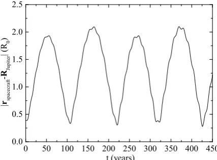
We observe that the relativistic effects perturb the spacecraft in such a way that its distance to the Sun is increased by several kilometers just ten or twenty years after the beginning of the experiment. This is within the range of radar measurements and could provide an extra test of general relativity and the validity of the post-Newtonian approximation. It is also important to check if a collision with Jupiter may happen in the future. To check that, we plotted the distance of the spacecraft to Jupiter in Figure5. We see that, although this distance varies periodically, a collision is not expected in the near future after the placement of the spacecraft in its initial orbit. The period of the oscillations in the distance of the spacecraft to Jupiter is, approximately, 110 years and it provides another way of exploring the richness of the resonant behavior.

0 50 100 150 200 250 300 350 400 450

0.0 0.5 1.0 1.5 2.0 2.5 | r s p a c e c r a f t -R J u p i t e r | ( R 0 ) t (years)

(8)

In Figure6we also plotted the amount of the relativistic contribution to the distance between of the spacecraft and Jupiter. We see that this contribution reaches increasing peaks in the range of a hundreds of kilometers. This contribution could be more easily detected if measurements were performed from another spacecraft in orbit around Jupiter or a radio antenna located at a Galilean moon.

0 50 100 150 200 250 300 350 400

Figure 6.Relative differences of the distances of the spacecraft to Jupiter (relativistic prediction minus Newtonian prediction) in the same conditions as those of Figure4.

It would be also interesting to consider another case in which the spacecraft is placed initially even closer to Jupiter. We expect that the chaotic behavior would emerge earlier in these circumstances. In Figure7, we plotted the distance of the spacecraft to the Sun forφ=−π/32 both for the Newtonian prediction and the relativistic one.

0 50 100 150 200 250 300 350 400

0.3 0.4 0.5 0.6 0.7 0.8 0.9 1.0 1.1 | r S u n ,s p a c e c r a f t | ( R 0 ) t (years)

Figure 7.Distance of the spacecraft to the Sun forφ=−π/32: Newtonian prediction (black line) and

the relativistic one (blue line).

(9)

0 10 20 30 40 50 60 70 -30

-20 -10 0 10 20 30

|

r

'

S

u

n

,

s

p

a

c

e

c

r

a

f

t

|

-|

r

S

u

n

,

s

p

a

c

e

c

r

a

f

t

|

(

km

)

t (years)

Figure 8. Difference between the distances of the spacecraft to the Sun as predicted for the post-Newtonian and post-Newtonian approximations in a resonant 1:1 orbit withφ=−π/32. Integration by the

Runge–Kutta order four method (solid line) and the fourth order Adams predictor-corrector method (open circles).

Here we see that variations of the order of 30 kms are expected in a period of ten years. This could provide a reliable, and relatively fast source of data to test the post-Newtonian approximations of general relativity in addition to the Messenger mission to Mercury and similar planetary missions [39]. Numerical Methods

In order to check the robustness of our results for the different initial conditions we discussed in the previous sections, we used different numerical methods for the integration of the equations of motion in the Newtonian and relativistic cases. Despite sensitivity to the initial conditions being high in this system, if the accuracy of the integration is improved by performing calculations in double, or even single precision we found that all methods agree in their predictions for the time domain of interest in this work.

Standard Runge–Kutta methods are the most obvious choice as they are implemented in many software packages [40]. As an alternative, that preserves the symplecticity of the Hamiltonian, we used the symplectic partitioned Runge–Kutta methods [41]. The properties of this method allows for the integration of larger times with a larger initial time-step. Notwithstanding these advantages, it was not clear how to implement it in the relativistic case, so we checked only the agreement with the typical Runge–Kutta of order four in the non-relativistic model.

Finally, for the relativistic equations of motion, we have compared them with the four-step Adams predictor-corrector method—a combination of the Adams–Bashforth and Adams–Moulton methods [42]. Predictor-corrector methods are explicit methods that combine two iterations per step. In the first one, we predict a new value of the coordinates (the so-called predictor algorithm) and in the second one the predicted value is corrected (the correction algorithm). The main inconvenience of this method is that we need the initial value of the spatial coordinates and velocities for time steps nhandn=0, . . . , 3 (in the four-order method). These initial values can be provided by the standard Runge–Kutta algorithm.

If the total relativistic accelerations are written asAx(t,px,py,qx,qy)andAy(t,px,py,qx,qy)for thexandycomponents, we can write the algorithm for the predictor step of theqxandpxcoordinates as follows:

¯

qx,n = qx,n+ h

24(55px,n−59px,n−1+37px,n−2−9px,n−3) , ¯

px,n = px,n+ h

24 55Ax(tn,px,n,py,n,qx,n,qy,n)−59Ax(tn−1,px,n−1,py,n−1,qx,n−1,qy,n−1) + 37Ax(tn−2,px,n−2,py,n−2,qx,n−2,qy,n−2)−9Ax(tn−3,px,n−3,py,n−3,qx,n−3,qy,n−3) .

(10)

Then, the corrector step is applied in the following form:

qx,n+1 = qx,n+ h

24(9 ¯px,n+19px,n−5px,n−1+px,n−2) , px,n+1 = px,n+ h

24 9Ax(tn+1, ¯px,n, ¯py,n, ¯qx,n, ¯qy,n) +19Ax(tn,px,n,py,n,qx,n,qy,n)

− 5Ax(tn−1,px,n−1,py,n−1,qx,n−1,qy,n−1) +Ax(tn−2,px,n−2,py,n−2,qx,n−2,qy,n−2)

. (8)

And similar equations should be used for the components in theycoordinate. In Equations (7) and (8),ndenotes then-th time step andtn =nh,hbeing the size of the time step. In our implementation of the method we tookh = 10−4in units ofτ = T0/(2π)withT0, the revolution period of Jupiter around the Sun. Being not natively supported by software packages such as Mathematica, this method is far more time consuming than the Runge–Kutta or the symplectic Runge–Kutta. In Figure8we show the results of both the fourth order Runge–Kutta method and the four-step Adams predictor-corrector method for the relativistic prediction of the distance of the spacecraft to the Sun in the resonant 1:1 orbit withφ=−π/32. We took the initial conditions for the Adams method from the Runge–Kutta method and single precision accuracy was used. A very good agreement was obtained between the two methods, save for discrepancies around five per cent that can be ascribed to rounding errors.

4. Conclusions

Testing general relativity has been a lengthy and complicated process, mainly as a consequence of the small effects involved, because gravity is the weakest of all forces in nature [43,44]. One of the main predictions of the theory, i.e., gravity waves, have only been directly detected very recently [45,46], just a century after general relativity was cast into its final form by Einstein. Anyway, it is surprising, in a certain sense, that even in the local environment of the Solar System there are tests that have not been completed to the precision required. Particularly, the problem of the relativistic contributions to the precision of the longitude of the ascending node and the argument of the pericenter of bodies orbiting around a rotating planet, also known as Lense–Thirring effect, is still a controversial subject [47–54].

These effects, however, are restricted to ideal situations on the ideal assumptions of the two-body problem. The implication of general relativity to the large-scale evolution of the N-body problem constituted by the Sun and all the planets, moons, and asteroids of the Solar System is still a major challenge in what concerns the confrontation of the theory with the observations. In the last decades, we have seen a startling development in the analysis of the large-scale evolution of the Solar System for periods of time in the range of millions of years. Laskar and collaborations [20,22] have shown that the long time regime of the Solar System is chaotic and that considerable fluctuations in the eccentricity and other orbital parameters are predicted for the inner planets for a period of the order of magnitude of the age of the Solar System. To perform the simulations for such long periods of time it has been necessary to employ symplectic methods of integration with the adequate properties of the absent secular terms in the energy integral, time reversibility, and angular momentum conservation [25,41].

These phenomena are particularly well evidenced for resonant orbits. An asteroid (or spacecraft) is said to be in resonance with a major planet when it completes its orbital period around the Sun; then, it is in a rational proportion with that of the major planet. Jupiter, being the largest and closer gaseous giant planet of the Solar System, is the main cause of resonances in the inner Solar System. These resonances have consequences for the stability of the asteroid belt in the end, and it is known to be responsible for the absence of asteroids with orbital periods in proportions 4:1, 3:1, 5:2, 7:3, and 2:1 with that of Jupiter. These are the, so-called, Kirkwood gaps. The destabilizing mechanism that induces the migration of asteroids from these orbits is still to be elucidated in detail, although a source of classical chaos was found in simulations by several authors [16–18].

(11)

resonance 2:1 or 1:1 with Jupiter where the perturbations by the giant planet would be very large. Monitoring the location and velocity of this spacecraft by Doppler and radar ranging would allow us to have a clear picture of the evolution of a resonant orbit in its early stages. In addition, it would also allow us to test the contribution of the relativistic effects to the large scale evolution of the Solar System. The post-Newtonian approximation of Einstein–Infeld–Hoffman seems entirely adequate for the analysis of the relativistic contributions, as gravitational radiation reaction can be neglected in the weak field and low velocities regime we are considering.

We found that, even when the classical Newtonian trajectory seems regular, the relativistic contributions add a source of non-periodicity to the ephemeris, as expected from chaotic dynamics. This can be traced even in a period of several years, or decades after launch, because the fluctuations in the position, for example, can be as large as 10 km. This would provide an experimental tool to evaluate the quality of the post-Newtonian approximation in a three-body problem, as realized by the interactions of the spacecraft with the Sun and Jupiter. Furthermore, it would provide an insight into the evolution and stability of the Solar System in both the past and the future.

We conclude that at the present stage of detailed analysis of the predictions of general relativity, a mission to study resonances and the associated relativistic effects may be worthwhile. The information derived from this study would help to establishing the validity of post-Newtonian mechanics and to probing the resonant perturbations on the human timescale or the role of relativity in the chaotic evolution of the Solar System and its stability.

Funding:This research received no external funding.

Acknowledgments:The author gratefully acknowledges Lluís Bel for some useful comments.

Conflicts of Interest:The author declares no conflict of interest.

References

1. Anderson, J.D.; Nieto, M.M. Astrometric Solar-System Anomalies. InRelativity in Fundamental Astronomy:

Dynamics, Reference Frames, and Data Analysis, Proceedings IAU Symposium; Seidelmann, P.K., Soffel, M., Eds.;

Cambridge University Press: Cambridge, UK, 2010; Volume 261, p. 189.

2. Iorio, L. Gravitational anomalies in the solar system? Int. J. Mod. Phys. D2015,24, 15300–15343. [CrossRef] 3. Iorio, L. On the anomalous secular increase of the eccentricity of the orbit of the Moon. Mon. Not. R. Astron.

Soc.2011,415, 1266–1275. [CrossRef]

4. Iorio, L. An Empirical Explanation of the Anomalous Increases in the Astronomical Unit and the Lunar Eccentricity.Astron. J.2011,142, 68. [CrossRef]

5. Anderson, J.D.; Campbell, J.K.; Ekelund, J.E.; Ellis, J.; Jordan, J.F. Anomalous Orbital-Energy Changes Observed during Spacecraft Flybys of Earth.Phys. Rev. Lett.2008,100, 091102. [CrossRef] [PubMed] 6. Turyshev, S.G.; Toth, V.T. The Pioneer Anomaly.Liv. Rev. Relat.2010,13, 4. [CrossRef]

7. Turyshev, S.G.; Toth, V.T.; Ellis, J.; Markwardt, C.B. Support for temporally-varying behavior of the Pioneer anomaly from the extended Pioneer 10 and 11 Doppler data sets. Phys. Rev. Lett. 2011, 107, 081103. [CrossRef]

8. Turyshev, S.G.; Toth, V.T.; Kinsella, G.; Lee, S.C.; Lok, S.M.; Ellis, J. Support for the thermal origin of the Pioneer anomaly.Phys. Rev. Lett.2012,108, 241101. [CrossRef]

9. Corda, C. Interferometric Detection of Gravitational Waves: The Definitive Test for General Relativity.Int. J.

Mod. Phys. D2009,18, 2275–2282. [CrossRef]

10. Kirkwood, D. On the theory of meteors. Proc. Am. Assoc. Adv. Sci.1866,15, 8–14.

11. Hedman, M.M.; Nicholson, P.D.; Baines, K.H.; Buratti, B.J.; Sotin, C.; Clark, R.N.; Brown, R.H.; French, R.G.; Marouf, E.A. The Architecture of the Cassini Division.Astron. J.2010,139, 228–251. [CrossRef]

12. Levison, H.F.; Morbidelli, A.; Van Laerhoven, C.; Gomes, R.; Tsiganis, K. Origin of the structure of the Kuiper belt during a dynamical instability in the orbits of Uranus and Neptune. Icarus2008,196, 258–273. [CrossRef]

(12)

14. Marcy, G.W.; Butler, R.P.; Fischer, D.; Vogt, S.S.; Lissauer, J.J.; Rivera, E.J. A Pair of Resonant Planets Orbiting GJ 876.Astrophys. J.2001,556, 296–301. [CrossRef]

15. Mills, S.M.; Fabrycky, D.C.; Migaszewski, C.; Ford, E.B.; Petigura, E.; Isaacson, H. A resonant chain of four transiting, sub-Neptune planets. Nature2016,533, 509–512. [CrossRef]

16. Lemaitre, A.; Henrard, J. On the origin of chaotic behavior in the 2/1 Kirkwood Gap.Icarus1990,83, 391–409. [CrossRef]

17. Morbidelli, A.; Moons, M. Secular resonances in mean motion commensurabilities—The 2/1 and 3/2 cases.

Icarus1993,102, 316–332. [CrossRef]

18. Morbidelli, A. The Kirkwood Gap at the 2/1 Commensurability With Jupiter: New Numerical Results.

Astron. J.1996,111, 2453. [CrossRef]

19. Morbidelli, A.; Zappala, V.; Moons, M.; Cellino, A.; Gonczi, R. Asteroid Families Close to Mean Motion Resonances: Dynamical Effects and Physical Implications. Icarus1995,118, 132–154. [CrossRef]

20. Laskar, J.; Quinn, T.; Tremaine, S. Confirmation of resonant structure in the solar system.Icarus1992,95, 148–152. [CrossRef]

21. Laskar, J. A numerical experiment on the chaotic behaviour of the solar system. Nature1989,338, 237. [CrossRef]

22. Laskar, J. Is the Solar System Stable? InChaos, Progress in Mathematical Physics; Springer-Verlag: Basel, Switzerland, 2013; Volume 66, pp. 239–270.

23. Kinoshita, H.; Yoshida, H.; Nakai, H. Symplectic integrators and their application to dynamical astronomy.

Celest. Mech. Dyn. Astron.1991,50, 59–71. [CrossRef]

24. Hayes, A.P. The Adams-Bashforth-Moulton Integration Methods Generalized to an Adaptive Grid.arXiv

2011, arXiv:1104.3187.

25. Geng, S. Symplectic partitioned Runge–Kutta methods. J. Comput. Math.1993,11, 365–372.

26. Lieske, J.H.Computer-Calculated Newtonian Ephemerides, 1800-2000, for Nine Principal Planets—Development

Ephemeris Number 28; Technical Report 32-1206; Jet Propulsion Laboratory, California Institute of Technology:

Pasadena, CA, USA, 1967.

27. Pitjeva, E.V.; Pitjev, N.P. Development of planetary ephemerides EPM and their applications. Celest. Mech.

Dyn. Astron.2014,119, 237–256. [CrossRef]

28. Iorio, L. Editorial for the Special Issue 100 Years of Chronogeometrodynamics: The Status of the Einstein’s Theory of Gravitation in Its Centennial Year.Universe2015,1, 38–81. [CrossRef]

29. Debono, I.; Smoot, G.F. General Relativity and Cosmology: Unsolved Questions and Future Directions.

Universe2016,2, 23. [CrossRef]

30. Vishwakarma, R. Einstein and Beyond: A Critical Perspective on General Relativity. Universe2016,2, 11. [CrossRef]

31. Fock, V.The Theory of Space, Time and Gravitation; Pergamon: Oxford, UK, 1964.

32. Landau, L.D.; Lifshitz, E.M.The Classical Theory of Fields, 4th ed.; Butterworth-Heinemann: Oxford, UK, 1980. 33. Einstein, A.; Infeld, L.; Hoffmann, B. The Gravitational equations and the problem of motion.Ann. Math.

1938,39, 65–100. [CrossRef]

34. Will, C.M. Inaugural Article: On the unreasonable effectiveness of the post-Newtonian approximation in gravitational physics.Proc. Natl. Acad. Sci. USA2011,108, 5938–5945. [CrossRef]

35. Brumberg, V. On derivation of EIH (Einstein–Infeld–Hoffman) equations of motion from the linearized metric of general relativity theory. Celest. Mech. Dyn. Astron.2007,99, 245–252. [CrossRef]

36. Will, C.M. New General Relativistic Contribution to Mercury’s Perihelion Advance. Phys. Rev. Lett.

2018,120, 191101. [CrossRef] [PubMed]

37. Iorio, L. The post-Newtonian gravitomagnetic spin-octupole moment of an oblate rotating body and its effects on an orbiting test particle; are they measurable in the Solar system? Mon. Not. R. Astron. Soc.

2019,484, 4811–4832. [CrossRef]

38. Misner, C.W.; Thorne, K.S.; Wheeler, J.A.Gravitation; Princeton University Pres: Princeton, NJ, USA, 1973. 39. Verma, A.K.; Fienga, A.; Laskar, J.; Manche, H.; Gastineau, M. Use of MESSENGER radioscience data to

improve planetary ephemeris and to test general relativity.Astron. Astrophys.2014,561, A115. [CrossRef] 40. Wolfram, S.The Mathematica Book, 5th ed.; Wolfram Media, Inc.: Champaign, IL, USA, 2003.

41. Blanes, S.; Moan, P. Practical symplectic partitioned Runge–Kutta and Runge–Kutta–Nystrom methods.

(13)

42. Goldstine, H.H. A History of Numerical Analysis from the 16th through the 19th Century; Springer-Verlag: New York, NY, USA, 1977.

43. Will, C.M. The confrontation between general relativity and experiment.Ann. N. Y. Acad. Sci.1980,336, 307–321. [CrossRef]

44. Will, C.M. The Confrontation between General Relativity and Experiment. Liv. Rev. Relat. 2006,9, 3. [CrossRef]

45. Abbott, B.P.; Abbott, R.; Abbott, T.D.; Abernathy, M.R.; Acernese, F.; Ackley, K.; Adams, C.; Adams, T.; Addesso, P.; Adhikari, R.X.; et al. Observation of Gravitational Waves from a Binary Black Hole Merger.

Phys. Rev. Lett.2016,116, 061102. [CrossRef]

46. Cervantes-Cota, J.; Galindo-Uribarri, S.; Smoot, G. A Brief History of Gravitational Waves.Universe2016,2, 22. [CrossRef]

47. Ciufolini, I.; Paolozzi, A.; Pavlis, E.C.; Ries, J.C.; Koenig, R.; Matzner, R.A.; Sindoni, G.; Neumayer, H. Towards a One Percent Measurement of Frame Dragging by Spin with Satellite Laser Ranging to LAGEOS, LAGEOS 2 and LARES and GRACE Gravity Models. Space Sci. Rev.2009,148, 71–104. [CrossRef]

48. Iorio, L. Some considerations on the present-day results for the detection of frame-dragging after the final outcome of GP-B.EPL (Europhys. Lett.)2011,96, 30001. [CrossRef]

49. Renzetti, G. Are higher degree even zonals really harmful for the LARES/LAGEOS frame-dragging experiment?Can. J. Phys.2012,90, 883–888. [CrossRef]

50. Renzetti, G. History of the attempts to measure orbital frame-dragging with artificial satellites. Cent. Eur.

J. Phys.2013,11, 531–544. [CrossRef]

51. Renzetti, G. Some reflections on the Lageos frame-dragging experiment in view of recent data analyses.

New Astron.2014,29, 25–27. [CrossRef]

52. Iorio, L.; Lichtenegger, H.I.M.; Ruggiero, M.L.; Corda, C. Phenomenology of the Lense-Thirring effect in the solar system. Astrophys. Space Sci.2011,331, 351–395. [CrossRef]

53. Iorio, L. Analytically calculated post-Keplerian range and range-rate perturbations: The solar Lense-Thirring effect and BepiColombo. Mon. Not. R. Astron. Soc.2018,476, 1811–1825. [CrossRef]

54. Lucchesi, D.M.; Anselmo, L.; Bassan, M.; Magnafico, C.; Pardini, C.; Peron, R.; Pucacco, G.; Visco, M. General Relativity Measurements in the Field of Earth with Laser-Ranged Satellites: State of the Art and Perspectives.

Universe2019,5, 141. [CrossRef]

c