Mapping of soil properties at high resolution in Switzerland using boosted geoadditive models

(1)

https://doi.org/10.5194/soil-3-191-2017

SOIL

Mapping of soil properties at high resolution in

Switzerland using boosted geoadditive models

Madlene Nussbaum1, Lorenz Walthert2, Marielle Fraefel2, Lucie Greiner3, and Andreas Papritz1

1_{Institute of Biogeochemistry and Pollutant Dynamics, ETH Zurich,}

Universitätstrasse 16, 8092 Zürich, Switzerland

2_{Swiss Federal Institute for Forest, Snow and Landscape Research (WSL),}

Zürcherstrasse 111, 8903 Birmensdorf, Switzerland

3_{Research Station Agroscope Reckenholz-Taenikon ART,}

Reckenholzstrasse 191, 8046 Zürich, Switzerland

Correspondence to:Madlene Nussbaum ([email protected])

Received: 7 April 2017 – Discussion started: 19 April 2017

Revised: 11 September 2017 – Accepted: 7 October 2017 – Published: 16 November 2017

Abstract. High-resolution maps of soil properties are a prerequisite for assessing soil threats and soil functions and for fostering the sustainable use of soil resources. For many regions in the world, accurate maps of soil properties are missing, but often sparsely sampled (legacy) soil data are available. Soil property data (response) can then be related by digital soil mapping (DSM) to spatially exhaustive environmental data that describe soil-forming factors (covariates) to create spatially continuous maps. With airborne and space-borne remote sensing and multi-scale terrain analysis, large sets of covariates have become common. Building parsimonious models amenable to pedological interpretation is then a challenging task.

We propose a new boosted geoadditive modelling framework (geoGAM) for DSM. The geoGAM models smooth non-linear relations between responses and single covariates and combines these model terms additively. Residual spatial autocorrelation is captured by a smooth function of spatial coordinates, and non-stationary effects are included through interactions between covariates and smooth spatial functions. The core of fully automated model building for geoGAM is component-wise gradient boosting.

(2)

1 Introduction

Soils fulfil many functions important for agriculture, forestry and the management of soil resources and natural hazards. The functionality of soils depends on their properties; hence, accurate and spatially highly resolved maps of basic soil properties such as texture, organic carbon content and pH for specific soil depth are needed for the sustainable man-agement of soils (FAO and ITPS, 2015). Unfortunately, such soil property maps are often missing and the availability of soil information is very different between nations and conti-nents (Omuto and Nachtergaele, 2013). For areas where spa-tially referenced but sparse (legacy) soil data are available, e.g. soil datasets consisting of soil profile data and labora-tory measurements, these point data can be linked using dig-ital soil mapping (DSM) techniques (e.g. McBratney et al., 2003; Scull et al., 2003) to spatial information on soil forma-tion factors to generate spatially continuous maps.

In the past, many DSM approaches have been proposed to exploit the correlation between soil properties (response Y(s)) and soil-forming factors (covariates x(s)). Linear re-gression modelling (LM; e.g. Meersmans et al., 2008; Hengl et al., 2014) and kriging with external drift (EDK), its ex-tension for autocorrelated errors (Bourennane et al., 1996; Nussbaum et al., 2014), have often been used. The strength of LM and EDK is the ease of interpretation of the fitted models (e.g. through partial residual plots; Faraway, 2005, p. 73). This is important for checking whether modelled re-lations between the target soil property and soil-forming fac-tors accord with pedological expertise and for conveying the results of DSM analyses to users of such products. LM and EDK capture only linear relations between the covariates and a response. By using interactions between covariates, one can sometimes account for non-linear relationships, but this quickly becomes unwieldy for a large number of covariates (e.g. above 30). Fitting models to (very) large sets of covari-ates has become common with the advent of remotely sensed data (Ben-Dor et al., 2009; Mulder et al., 2011) and novel approaches for terrain analysis (Behrens et al., 2010). Model building, i.e. covariate selection, is then a formidable task. Although specialised methods like L2-boosting (Bühlmann and Hothorn, 2007) and lasso (least absolute shrinkage and selection operator; Hastie et al., 2009, Chap. 3) are available, they have not often been used for DSM (Nussbaum et al., 2014; Liddicoat et al., 2015; Fitzpatrick et al., 2016). Gener-alised linear models (GLMs; e.g. Dobson, 2002) extend lin-ear modelling to binary, nominal (e.g. soil taxonomic units; Hengl et al., 2014; Heung et al., 2016) or ordinal responses (e.g. soil drainage classes; Campling et al., 2002). Although GLMs are non-linear models, the non-linearly transformed conditional expectationg(E[Y(s)|x(s)]), whereg(·) is some known link function, still depends linearly on covariates.

Lately, tree-based machine learning methods have be-come popular for DSM. Classification and regression trees (CARTs; e.g. Liess et al., 2012; Heung et al., 2016), Cubist

(e.g. Henderson et al., 2005; Adhikari et al., 2013; Lacoste et al., 2016) and ensemble tree methods like random forest (RF; e.g. Grimm et al., 2008; Wiesmeier et al., 2011) and boosted regression trees (BRTs; e.g. Moran and Bui, 2002; Martin et al., 2011) have been used.

All tree-based methods easily account for complex non-linear relations between responses and covariates. They model continuous and categorical responses (albeit without making a difference between nominal and ordinal responses), inherently deal with incomplete covariate data and allow for the modelling of spatially changing (non-stationary) relation-ships. BRT and RF fit models to large sets of covariates. The structure of the fitted models can be explored with variable importance and partial dependence plots (Hastie et al., 2009, Sect. 10.9, and for an application Martin et al., 2011). Never-theless, tree-based ensemble methods remain complex, and results are not as easy to interpret regarding the relevant soil-forming factors resulting from (G)LM.

Generalised additive models (GAMs; e.g. Hastie and Tib-shirani, 1990, Chap. 6) offer a compromise between ease of interpretation and flexibility in modelling non-linear relation-ships. GAMs expand the (possibly transformed) conditional expectation of a response given covariates as an additive se-ries:

gE

Y(s)|x(s)₌

ν+f x(s)₌

ν+X

j

fj xj(s), (1)

whereνis a constant, andfj xj(s)values are linear terms or unspecified “smooth” non-linear functions of single covari-atesxj(s) (e.g. smoothing spline, kernel or any other scatter plot smoother) andg(·) is again a link function. GAMs ex-tend GLMs to account for truly non-linear relations between Y andx(and not just for non-linearities imposed byg), but they limit the complexity of the fitted functions to additive combinations of simple non-linear terms and thereby avoid the curse of dimensionality (Hastie et al., 2009, Sect. 2.5). For continuous, ordinal and nominal responses, GAMs can be readily fitted to large sets of covariates through boost-ing (Hofner et al., 2014; Hothorn et al., 2015). Boostboost-ing handles covariate selection and avoids over-fitting if stopped early (Bühlmann and Hothorn, 2007). Hence, the structure of boosted GAMs can be more easily checked and interpreted than RF and BRT models. In the past, GAMs have occasion-ally been used for DSM and only recently became more pop-ular (e.g. Buchanan et al., 2012; Poggio et al., 2013; Poggio and Gimona, 2014; de Brogniez et al., 2015; Sindayihebura et al., 2017).

(3)

from model building is ignored. To take the effect of model building properly into account one resorts best to bootstrap-ping (Davison and Hinkley, 1997, Sect. 6.3.3). Bootstrapbootstrap-ping is also useful to model prediction uncertainty for boosted models, which do not qualify the accuracy of predictions per se, and to account for all sources of prediction un-certainty in regression kriging approaches (Viscarra Rossel et al., 2014).

In summary, a versatile DSM procedure should

1. model non-linear relations betweenY(s) andx(s), where responses and covariates may be continuous, binary, nominal or ordinal variables,

2. efficiently build models with good predictive perfor-mance for large sets of covariates (p>>30),

3. preferably result in parsimonious models with a simple structure that can be easily interpreted and checked for plausibility, and

4. accurately quantify the accuracy of predictions com-puted from the fitted models.

The objective of our work was to develop a DSM frame-work that meets requirements 1–4 based on boosted geoad-ditive models (geoGAMs), an extension of GAM for spatial data. First, we introduce the modelling framework and de-scribe in detail the model-building procedure. Second, we use the method in three DSM case studies in the Canton of Zurich, Switzerland that aim at different types of responses: effective cation exchange capacity (ECEC) of forest topsoils (continuous response), the presence or absence of morpho-logical features for waterlogging in agricultural soils (binary response) and drainage classes characterising the prevalence of anoxic conditions, again in agricultural soils (ordinal re-sponse). To assess the validity of the modelling results with independent data (obtained by splitting the original dataset into calibration and validations subsets), we used specific cri-teria that take the nature of the various responses properly into account. These criteria are in common use for forecast verification in atmospheric sciences (e.g. Wilks, 2011), but to our knowledge have not often been used to (cross-)validate DSM predictions.

2 The geoGAM framework

2.1 Model representation

A generalised additive model (GAM) is based on the fol-lowing components (Hastie and Tibshirani, 1990, Chap. 6 and Eq. 1). (i) Response distribution: given x(s)=

x1(s), x2(s), . . . , xp(s) T

, theY(s) values are conditionally independent observations from simple exponential family distributions. (ii) Link function: g(·) relates the expectation µ x(s)=EY(s)|x(s) of the response distribution to (iii) the additive predictorP

jfj xj(s)

.

GeoGAM extends GAM by allowing for a more complex form of the additive predictor (Kneib et al., 2009; Hothorn et al., 2011). First, one can add a smooth functionfs(s) of

the spatial coordinates (smooth spatial surface) to the addi-tive predictor to account for residual autocorrelation. More complex relationships betweenY andxcan be modelled by adding terms likefj xj(s)·fk xk(s)to capture the effect of interactions between covariates andfs(s)·fj xj(s)to ac-count for the spatially changing dependence betweenY and x. Hence, in its full generality, a generalised additive model for spatial data is represented by

g µ x(s)

=ν+f x(s)

=ν+X

u

fju xju(s)

+X

v

fjv xjv(s)

·fkv xkv(s)

| {z }

global marginal and interaction effects

+X

w

fsw(s)·fjw xjw(s)

| {z }

non-stationary effects

+ fs(s)

| {z }

autocorrelation

. (2)

Kneib et al. (2009) called Eq. (2) a geoadditive model, a name coined before by Kammann and Wand (2003) for a combination of Eq. (1) with a geostatistical error model.

It remains to be specified what response distributions and link functions should be used for the various response types. For (possibly transformed) continuous responses, one often uses a normal response distribution combined with the iden-tity linkg µ(x(s))=µ x(s). For binary data (coded as 0 and 1), one assumes a Bernoulli distribution and often uses a logit link:

g(µ(x(s)))=log

µ(x(s)) 1−µ(x(s))

, (3)

where

µx(s)

=ProbY(s)=1|x(s)

= exp ν+f x(s)

1+exp ν+f x(s). (4)

For ordinal data with ordered response levels, 1,2, . . . , k, we used the cumulative logit or proportional odds model (Tutz, 2012, Sect. 9.1). For any given levelr∈(1,2, . . . , k), the logarithm of the odds of the eventY(s)≤r|x(s) is then modelled by

log Prob

Y(s)≤r|x(s)

Prob

Y(s)> r|x(s) !

=νr+f x(s)

, (5)

withνra sequence of level-specific constants satisfyingν1≤

ν2≤. . .≤νr. Conversely,

Prob

Y(s)≤r|x(s)

= exp νr

+f x(s)

1+exp νr+f x(s)

. (6)

Note that Prob

Y(s)≤r|x(s)

depends onronly through the constantνr. Hence, the ratio of the odds of two eventsY(s)≤

r|x(s) andY(s)≤r|

ex(s) is the same for all r (Tutz, 2012,

(4)

2.2 Model building (selection of covariates)

To build parsimonious models that can readily be checked for agreement with pedological understanding, we applied a sequence of fully automated steps 1–6. In several of these steps we optimised tuning parameters through 10-fold cross-validation with fixed subsets using root mean square error (RMSE; Eq. (12), continuous responses), Brier score (BS; Eq. (16), binary responses) or ranked probability score (RPS; Eq. (18), ordinal responses) as optimisation criteria. Model building aims to optimise the accuracy of predictions, and hence we did not use equivalent “goodness-of-fit” statistics. To improve the stability of the algorithm continuous covari-ates were first scaled (by the difference of the maximum and minimum value) and centred.

1. Boosting (see step 2 below) is more stable and con-verges more quickly when the effects of categorical co-variates (factors) are accounted for as a model offset. We therefore used the group lasso (Breheny and Huang, 2015) – an algorithm that likely excludes non-relevant covariates and treats factors as groups – to select impor-tant factors for the offset. For ordinal responses (Eq. 6) we used stepwise proportional odds logistic regression in both directions with BIC (e.g. Faraway, 2005, p. 126) to select the offset covariates because lasso cannot be used for such responses.

2. Next, we selected a subset of relevant factors, continu-ous covariates and spatial effects by using component-wise gradient boosting. Boosting is a slow stage-component-wise additive learning algorithm. It expandsf x(s)

in a set of base procedures (base learners) and approximates the additive predictor by using a finite sum of them as fol-lows (Bühlmann and Hothorn, 2007).

(a) Initialisefˆx(s)[m]

with the offset of step 1 above and setm=0.

(b) Increase m by 1. Compute the negative gradient vectorU[m]_{(e.g. residuals) for a loss function}_l₍_·_). (c) Fit all base learners fj xj(s), j=1, . . . , p to

U[m] _{and select the base learner, for example} fk(xk(s))[m], that minimizesl(·).

(d) Updatefˆx(s)[m]_{= ˆ}

f x(s)[m−1]₊

v·fk xk(s) [m]

with step sizev≤1.

(e) Iterate steps (b) to (d) untilm=mstop(main tuning

parameter).

We used the following settings in the above algorithm. As loss functionsl(·) we usedL2for continuous,

neg-ative binomial likelihood for binary (Bühlmann and Hothorn, 2007) and proportional odds likelihood for or-dinal responses (Schmid et al., 2011). Early stopping of the boosting algorithm was achieved by determining optimalmstopthrough cross-validation. We used default

step length (υ=0.1). This is not a sensitive parameter as long as it is clearly below 1 (Hofner et al., 2014). For continuous covariates we used penalised smoothing spline base learners (Kneib et al., 2009). Factors were treated as linear base learners. To capture residual auto-correlation we added a bivariate tensor product P-spline of spatial coordinates (Wood, 2006, pp. 162) to the ad-ditive predictor. Spatially varying effects were modelled by using base learners formed through multiplication of continuous covariates with tensor product P-splines of spatial coordinates (Wood, 2006, pp. 168). An uneven degree of freedom of base learners biases base learner selection (Hofner et al., 2011). We therefore penalised each base learner to 5 degrees of freedom (df). Factors with fewer than six levels (df<5) were aggregated to grouped base learners. By using an offset, the effects of important factors with more than six levels were implic-itly accounted for without penalisation.

3. Atmstop(see step 2 above), many included base learners

had very small effects only. We fitted generalised addi-tive models (GAMs; Wood, 2011) and included smooth and factor effects only if their effect sizeej of the cor-responding base learnerfj(xj(s)) was substantial. The effect sizeej of factors was the largest difference be-tween the effects of two levels and for continuous co-variates it was equal to the maximum contrast of esti-mated partial effects (after the removal of extreme val-ues as in box plots; Frigge et al., 1989). We iterated throughejand excluded covariates withejsmaller than a threshold effect sizeet. Optimalet was determined by 10-fold cross-validation of GAM. In these GAM fits, smooth effects were penalised by 5 degrees of free-dom as imposed by component-wise gradient boosting (step 2 above). The factors selected as an offset in step 1 were now included in the GAM.

4. We further reduced the GAM through the stepwise removal of covariates by using cross-validation. The candidate covariate to drop was chosen by the largest p value of F tests for linear terms and approximate F tests (Wood, 2011) for smooth terms.

5. Factor levels with similar estimated effects were merged stepwise again through cross-validation based on the largestpvalues from two samplettests of partial resid-uals.

(5)

Model-building steps 1 to 6 were implemented in the R packagegeoGAM(Nussbaum, 2017).

2.3 Predictions and predictive distribution

Soil properties were predicted for new locations s+ from the final geoGAM by usingeY(s+)= ˆf x(s+). To model the predictive distributions for continuous responses we used a non-parametric, model-based bootstrapping approach (Davi-son and Hinkley, 1997, pp. 262, 285) as follows.

A. New values of the response were simulated according to Y(s)∗= ˆf x(s)+, wherefˆ x(s)represents the fitted values of the final model and values are errors ran-domly sampled with replacement from the centred, ho-moscedastic residuals of the final model (Wood, 2006, p. 129).

B. The geoGAM was fitted toY(s)∗_{according to steps 1–6} of Sect. 2.2.

C. Prediction errors were computed according to δ₊∗ = ˆ

f x(s+)

∗

−fˆ x(s+)

+, where fˆ(x(s+))∗ repre-sents predicted values at new locationss+of the model built with the simulated responseY(s)∗in step B above, and the errors are again randomly sampled from the centred, homoscedastic residuals of the final model (see step A).

Prediction intervals were computed according to

_ˆ

f x(s+)−δ∗+(1−α); ˆf x(s+)−δ+∗(α)

, (7)

whereδ₊∗₍_α₎andδ₊∗₍₁₋_α₎are theαand (1−α) quantiles of δ₊∗ pooled over all 1000 bootstrap repetitions.

Predictive distributions for binary and ordinal responses were directly obtained from the final geoGAM fit by predict-ing probabilities of occurrence Probg Y(s)=r|x(s)

(Davi-son and Hinkley, 1997, p. 358).

3 Case studies: materials and methods

3.1 Study regions

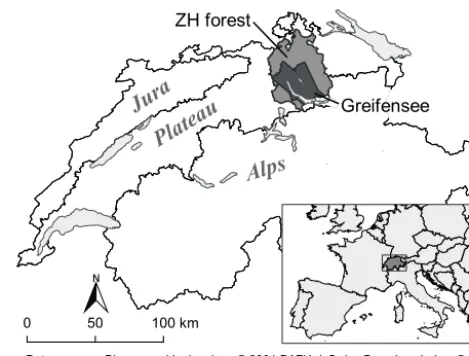
We applied the modelling framework to three datasets on properties of forest and agricultural soils in the Canton of Zurich in Switzerland (Fig. 1). Forests (ZH forest), as defined by the Swiss topographic landscape model (swissTLM3D, Swisstopo, 2013a), cover an area of 506.5 km2, or roughly 30 % of the total area of the Canton of Zurich. The spatial extent of the agricultural region near Greifensee was defined by the availability of imaging spectroscopy data collected by the APEX spectrometer (Schaepman et al., 2015). Agricul-tural land was defined as the area not covered by any areal features, such as settlements or forests, extracted from the Swiss topographic landscape model (swissTLM3D, Swis-stopo, 2013a). Wetlands, forests, parks or city gardens were excluded, resulting in a study region of 170 km2.

0 50 100 km

Ju

ra

Alps

Greifensee

Pla

tea

u

ZH forest

Figure 1.Location of the study regions Greifensee and ZH forest on the Swiss Plateau.

In the Canton of Zurich, forests extend across altitudes ranging from 340 to 1170 m above sea level (m. a.s.l), and in the Greifensee area elevation ranges from 390 to 840 m a.s.l. (Swisstopo, 2016). The climatic conditions (period 1961– 1990; Zimmermann and Kienast, 1999) vary accordingly, with mean annual rainfall of 880–1780 mm for the forested and 1040–1590 mm for the agricultural study region. Mean annual temperatures range between 6.1–9.1 and 7.5–9.1◦C, respectively. Two-thirds of the forested area is dominated by coniferous trees (FSO, 2000b). Half of the Greifensee study region is covered by cropland and one-third by permanent grassland. The remainder is comprised of orchards, horti-cultural areas or mountain pastures (Hotz et al., 2005). In the Canton of Zurich, soils are formed mostly from Molasse formations and Quaternary sediments dominantly from the last glaciation (Würm). In the north-eastern part, the lime-stone Jura hills reach into the ZH forest study region (Hantke, 1967).

3.2 Data

3.2.1 Soil database

(6)

sampling according to the aims of the project. Soil data were therefore quite heterogeneous, and tailored harmonisation procedures were required to provide consistent soil datasets. The heterogeneity resulted from several standards of soil de-scription and soil classification, different data keys, different analytical methods and, in particular, often missing metadata for a proper interpretation of the datasets. Therefore, we elab-orated a general harmonisation scheme that covers the main steps required to merge different soil legacy data into one common, consistent database (Walthert et al., 2016). Sam-pling sites were recorded in the field on topographic maps (scale 1 : 25 000), and hence we estimated the accuracy of coordinates to about±25 m.

3.2.2 Effective cation exchange capacity (ECEC, forest soils)

After the removal of sites with missing covariate values, we used 1844 topsoil samples from 1348 sites with data on effec-tive cation exchange capacity (ECEC). Most measurements refer to composite samples for which aliquots were measured in 20 m×20 m squares from 0–20 cm of soil depth. For about 100 sites, soil profile genetic horizons were sampled. ECEC [mmolckg−1] for 0–20 cm was computed from horizon data

by using

ECEC0−20= h

X

i=1

wiECECi, (8)

where ECECiis the value for horizoni,wiis a weight given by soil densityρiand the fraction of the thickness of horizon

iwithin 0–20 cm andhis the number of horizons intersect-ing the 0–20 cm depth; ρi was estimated from soil organic matter (SOM) and/or sampling depth by using a pedotrans-fer function (PTF; see the Supplement of Nussbaum et al., 2017). Due to a lack of respective data, the volumetric stone content was assumed to be constant.

For most soil samples, ECEC was measured after extrac-tion in an ammonium chloride soluextrac-tion (FAC, 1989; Walthert et al., 2004, 2013). Roughly 5 % of the samples had only measurements of Ca, Mg, K and Al (extracted by ammo-nium acetate EDTA solution; Lakanen and Erviö, 1971; ELF, 1996; Gasser et al., 2011). For these samples, we estimated ECEC by using a PTF (Nussbaum and Papritz, 2015).

We assigned 293 of 1348 sites (528 samples) to the valida-tion set, which was used to check the predictive performance of the fitted statistical model, and the remaining 1055 sites (1316 samples) were used to calibrate the model. The legacy samples were spatially clustered. To ensure that the valida-tion sites were evenly spread over the study region, the vali-dation sites were selected by weighted random sampling. The weight attributed to a site was proportional to the forested area within its Dirichlet polygon (Dirichlet, 1850).

We found a considerable variation in ECEC values ranging from 17.4 to 780 mmolckg−1 (median 141.1 mmolckg−1;

Table S1 in the Supplement). On average, ECEC was slightly larger in the calibration than in the validation set.

3.2.3 Presence of waterlogged soil horizons (agricultural soils)

Waterlogging characteristics were recorded in the field at 962 sites within the Greifensee study region by visual evaluation (Jäggli et al., 1998). Swiss soil classification distinguishes horizon qualifiers gg (strongly gleyic, predominantly oxi-dised) and r(anoxic, predominantly reduced) and both are believed to limit plant growth (Jäggli et al., 1998; Müller et al., 2007; Litz, 1998; Danner et al., 2003; Kreuzwieser and Rennberg, 2014).

We constructed binary responses for three soil depths: 0– 30 cm, 0–50 cm and 0–100 cm. If one of the horizon quali-fiersggorrwas recorded within the interval, we assigned 1 as thepresence of waterlogged horizonsand 0 as theabsence of waterlogged soil horizonsotherwise.

We chose 198 of 962 sites to form a validation set, again by using weighted random sampling. The remaining 764 sites were used to build and fit the models. In the topsoil (0–30 cm),ggorrhorizon qualifiers were only observed at 13.4 % of the 962 sites. Down to 50 cm, about twice as many sites (25.9 %) showed signs of anoxic conditions and down to 1 m 38.6 % of sites featured an anoxic or gleyic horizon (Table S2).

3.2.4 Drainage classes (agricultural soils)

Swiss soil classification differentiates the hydromorphic fea-tures of soils in more detail, describing the degree, depth and source of waterlogging with three supplementary qualifiers for stagnic, gleyic or anoxic profiles (I, G, R; categorical at-tributes, Brunner et al., 1997). To reduce the complexity of classification, we aggregated these qualifiers to three ordered levels:well drained(qualifiers I1–I2, G1–G3, R1 or no hy-dromorphic qualifier),moderately well drained (I3–I4, G4) andpoorly drained(G5–G6, R2–R5).

For validation we used the same 198 sites as for the

presence of waterlogged soil horizons, but only 732 sites were used for model building due to missing supplemen-tary qualifiers. The majority (66.6 %) of the 930 sites were

well drained, only 12.7 % were classified asmoderately well drainedand 20.7 % aspoorly drained(Table S3 in the Sup-plement).

3.2.5 Covariates for statistical modelling

(7)

agri-cultural drainage networks, resulting in 498 covariates in to-tal.

3.3 Statistical analysis

We built models for the five responses according to Sect. 2.2 and computed predictions for new locations at nodes of a 20 m grid. Predictions were post-processed as described in the following.

3.3.1 Response transformation

ECEC data for 0–20 cm of soil depth were positively skewed (Table S1); hence we fitted the model to the log-transformed data. In full analogy to log-normal kriging (Cressie, 2006, Eq. 20), the predictions were back-transformed by using

E

Y(s+)|x

=exp

ˆ f x(s+)

+1

2σˆ

2₋1

2Var

h

ˆ f x(s+)

i

,

(9)

with fˆx(s+) being the prediction of the log-transformed response,σˆ2the estimated residual variance of the final ge-oGAM fit and Var_ˆ

f x(s+) the variance of fˆ x(s+) as provided by the final geoGAM. Limits of prediction intervals were back-transformed by using exp(·) as they are quantiles of the predictive distributions.

3.3.2 Conversion of probabilistic to categorical predictions

For binary and ordinal responses, Eqs. (4) and (6) predict probabilities of the respective response levels. To predict the “most likely” outcome one has to apply a threshold to these probabilities. For binary data we predicted the presence of waterlogged horizonsif the probability exceeded the optimal value of the Gilbert skill score (GSS; Sect. 3.3.3) that dis-criminated between thepresenceandabsence of waterlogged horizonsbest in cross-validation of the final geoGAM. GSS was selected because the absence of waterlogged horizons

was more common thanpresence, especially in topsoil. To ensure consistency in the maps for sequential soil depths we assigned thepresence of waterlogged horizonsto the lower depth if it was predicted for the depth above.

For ordinal responses we predicted the level to which the median of the probability distribution Prob(g Y(s)≤r|x(s))

was assigned (Tutz, 2012, p. 475).

3.3.3 Evaluating the predictive performance of the statistical models

The predictive performance of the geoGAM, fitted for the continuous response ECEC, was tested by comparing predic-tionseY(si) (Eq. 9) with measurementsY(si) of independent

validation sets. Marginal bias and overall accuracy were as-sessed by using

BIAS= −1 n

n

X

i=1

(Y(si)−eY(si)), (10)

robBIAS= −median1≤i≤n Y(si)−eY(si), (11)

RMSE= 1 n

n

X

i=1

Y(si)−eY(si) 2

!1/2

, (12)

robRMSE=MAD1≤i≤n Y(si)−eY(si), (13)

SSmse=1−

Pn

i=1 Y(si)−eY(si) 2

Pn

i=1

Y(si)−1_nPni=1Y(si)

2, (14)

where MAD is the median absolute deviation. SSmsewas

de-fined as mean square error skill score (Wilks, 2011, p. 359) with the sample mean of the measurements as a refer-ence prediction method. Interpretation is similar toR2with SSmse =1 for perfect predictions and SSmse =0 for zero

explained variance. SSmsebecomes negative if the root mean

square error (RMSE) exceeds the standard deviation of the data. To validate the accuracy of the bootstrapped predictive distributions we plotted the empirical distribution function of the probability integral transform (Wilks, 2011, p. 375), which is equivalent to a plot of the coverage of one-sided prediction intervals 0,_eqα(s)

against the nominal probabili-tiesαused to construct the quantiles_eqα(s).

For binary responses the predictive performance of the fit-ted geoGAM was evaluafit-ted with independent validation data by using the Brier skill score (BSS; Wilks, 2011, Eq. 8.37):

BSS=1− BS BSref

, (15)

where the Brier score (BS) is computed with

BS=1 n

n

X

i=1

(yi−oi)2, (16)

wheren is the number of sites,yi=Probg

Y(si)=1|x(si)

represents the predicted probabilities andoi=I Y(si)=1

is the observation. BSrefis the BS of a reference prediction in

which the more abundant level (absence of waterlogged hori-zons) is always predicted. After transforming the predicted probabilities to the binary levels (presence or absence of wa-terlogged horizons; Sect. 3.3.2), we further evaluated the bias ratio, Peirce skill score (PSS) and GSS. The bias ratio is the ratio of the number ofpresencepredictions to the number ofpresenceobservations (Wilks, 2011, Eq. 8.10). PSS is a skill score based on the proportion of correctpresenceand

(8)

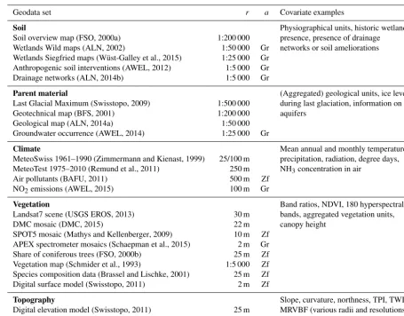
Table 1.Overview of geodata and derived covariates; for more information see the Supplement of Nussbaum et al. (2017); (r: pixel resolution for raster datasets or scale for vector datasets,a: only available for study region Greifensee (Gr) or ZH forest (Zf), NDVI: normalised differenced vegetation index, TPI: topographic position index, TWI: topographic wetness index, MRVBF: multi-resolution valley bottom flatness).

Geodata set r a Covariate examples

Soil Physiographical units, historic wetland

Soil overview map (FSO, 2000a) 1:200 000 presence, presence of drainage Wetlands Wild maps (ALN, 2002) 1:50 000 Gr networks or soil ameliorations Wetlands Siegfried maps (Wüst-Galley et al., 2015) 1:25 000 Gr

Anthropogenic soil interventions (AWEL, 2012) 1:5 000 Gr Drainage networks (ALN, 2014b) 1:5 000 Gr

Parent material (Aggregated) geological units, ice level Last Glacial Maximum (Swisstopo, 2009) 1:500 000 during last glaciation, information on Geotechnical map (BFS, 2001) 1:200 000 aquifers

Geological map (ALN, 2014a) 1:50 000

Groundwater occurrence (AWEL, 2014) 1:25 000 Gr

Climate Mean annual and monthly temperature, MeteoSwiss 1961–1990 (Zimmermann and Kienast, 1999) 25/100 m precipitation, radiation, degree days, MeteoTest 1975–2010 (Remund et al., 2011) 250 m NH3concentration in air

Air pollutants (BAFU, 2011) 500 m Zf

NO2emissions (AWEL, 2015) 100 m Gr

Vegetation Band ratios, NDVI, 180 hyperspectral Landsat7 scene (USGS EROS, 2013) 30 m bands, aggregated vegetation units,

DMC mosaic (DMC, 2015) 22 m canopy height

SPOT5 mosaic (Mathys and Kellenberger, 2009) 10 m Zf APEX spectrometer mosaics (Schaepman et al., 2015) 2 m Gr Share of coniferous trees (FSO, 2000b) 25 m Zf Vegetation map (Schmider et al., 1993) 1:5 000 Zf Species composition data (Brassel and Lischke, 2001) 25 m Zf Digital surface model (Swisstopo, 2011) 2 m Zf

Topography Slope, curvature, northness, TPI, TWI, Digital elevation model (Swisstopo, 2011) 25 m MRVBF (various radii and resolutions) Digital terrain model (Swisstopo, 2013b) 2 m

and again random predictions as a reference. Perfect pre-dictions have PSS and GSS equal to 1; for random predic-tions the scores are equal to 0 and predicpredic-tions worse than the reference receive negative scores. PSS is truly and GSS asymptotically equitable, meaning that purely random and constant predictions get the same scores (see Wilks, 2011, pp. 316 and 321 for details).

For the ordinal response drainage classes we tested the fit-ted geoGAM by evaluating the ranked probability skill score (RPSS), which was computed for the independent validation data analogously to BSS by using

RPSS=1− RPS RPSref

, (17)

where RPS is the ranked probability score (RPS; Wilks, 2011, Eq. 8.52) given by

RPS=

n

X

i=1 J

X

j=1

(Yi,j−Oi,j)2, (18)

with Yi,j=Probg

Y(si)≤j|x(si) being the pre-dicted cumulative probabilities up to class j and Oi,j=Pjr=1I Y(si)=r

indicating observed absence (0) or presence (1) up to class j. RPSref is the RPS for

a reference that always predicts the most abundant class (well drained). For predictions of the ordinal outcomes (Sect. 3.3.2) we also computed the mean bias ratio from three bias ratios created analogously to the binary case. These two-class settings were achieved through the stepwise aggregation of two out of three classes (wellvs.moderately well or poorly drained, then well or moderately well vs.

(9)

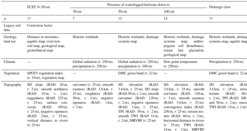
Table 2.Covariates contained in final geoGAM for responses ECEC, thepresence of waterlogged horizonsand drainage classes. More details on covariate effects can be found in Figs. S1 and S4 to S6 in the Supplement (p: number of covariates, SD: standard deviation in a moving window, RAD: radius of moving window or parameter of terrain attribute algorithm, r: resolution of elevation model, TPI: topographic position index, TWI: topographic wetness index, MRVBF: multiresolution valley bottom flatness).

ECEC 0–20 cm Presence of waterlogged horizons down to Drainage class

30 cm 50 cm 100 cm

p 17 7 12 14 11

Legacy soil data

Correction factor

Geology, land use

Distance to moraines, aquifer map, overview soil map, geological map, geotechnical map

Historic wetlands Historic wetlands, drainage systems map

Historic wetlands, drainage systems map, anthro-pogenic soil disturbance, extent last glaciation, geological map

Historic wetlands, drainage systems map, aquifer map

Climate — Global radiation (r: 250 m), precipitation (r: 250 m)

Global radiation (r: 250 m), precipitation (r: 100 m)

Dew point temperature (r: 250 m)

Precipitation (r: 250 m)

Vegetation SPOT5 vegetation index (r: 10 m), vegetation map

— DMC green band (r: 22 m) — DMC green band (r: 22 m)

Topography SD slope (RAD: 20 m, r: 2 m), smooth northness (RAD: 10 m, r: 2 m), ruggedness (RAD: 225 m, r: 25 m), surface con-vexity (RAD: 450 m, r: 25 m), negative openness (RAD: 2 km, r: 25 m), vertical distance to rivers (r: 25 m)

curvature (r: 25 m), smooth eastness (RAD: 3.6 km, r: 25 m), roughness (RAD: 50 m, r: 2 m), negative openness (RAD: 1 km, r: 2 m)

SD elevation (RAD: 3.6 km, r: 25 m), SD slope (RAD 50 m, r: 2 m), smooth curvature (RAD: 120 m, r: 2 m), negative openness (RAD: 1 km, r: 25 m), TPI (RAD: 50 m, r: 2 m), smooth TWI (RAD 14 m, r: 2 m), MRVBF (r: 25 m)

SD elevation (RAD: 3.6 km, r: 25 m), smooth curvature (RAD: 120 m, r: 2 m), smooth eastness (RAD: 3.6 km, r: 25 m), convergence index (RAD: 250 m, r: 25 m), terrain tex-ture (RAD: 60 m, r: 2 m), horizontal distance to rivers (r: 25 m), TWI (RAD: 14 m, r: 2 m), MRVBF (25 m)

SD elevation (RAD: 3.6 km, r: 25 m), terrain texture (RAD: 60 m, r: 2 m), TPI (RAD: 300 m and 50 m, r: 2 m), smooth TWI (RAD: 14 m, r: 2 m)

3.3.4 Software

Terrain attributes were computed by ArcGIS (version 10.2; ESRI, 2010) and SAGA 2.1.4 (version 2.1.4; Conrad et al., 2015). All statistical computations were performed in R (ver-sion 3.2.2; R Core Team, 2016) using several add-on pack-ages, in particular grpreg for group lasso (version 2.8-1; Breheny and Huang, 2015),MASSfor proportional odds logit regression (version 7.3-43; Venables and Ripley, 2002), mboostfor component-wise gradient boosting (version 2.5-0; Hothorn et al., 2015), mgcv for geoadditive model fits (version 1.8-6; Wood, 2011),rasterfor spatial data pro-cessing (version 2.4-15; Hijmans et al., 2015) andgeoGAM for the model-building routine (version 0.1-2; Nussbaum, 2017).

4 Results

4.1 ECEC – case study 1

4.1.1 Models for ECEC in 0–20cmof depth

Figure 2 shows the change in RMSE during model build-ing (10-fold cross-validation). The small root mean square error (RMSE) of 0.428 log mmolckg−1 after the gradient

boosting step – with coefficients shrunken by the algo-rithm – could further be reduced (cross-validation RMSE

0.422 log mmolckg−1) by removing covariates and through

factor aggregation. Aggregating factor levels resembles the shrinking of coefficients of such covariates.

Starting with 333 covariates, model building successfully reduced the number of covariates in the model to 17. The remaining ones characterised geology, vegetation and topog-raphy (Table 2). Effective cation exchange capacity (ECEC) depended non-linearly on nearly all continuous covariates, but non-linearities were in general rather weak (Fig. S1 in the Supplement). Nofs(s) term was included in the model

because residual autocorrelation was very weak (Fig. S2). Including non-stationary effects in the model would have improved the model only slightly (cross-validation RMSE 0.406 log mmolckg−1) but would have added considerable

complexity to the final model (21 covariates including eight interactions withfs(s) terms).

4.1.2 Validation of predicted ECEC with independent data

(10)

con-0.42 0.43 0.44 0.45 0.46 C ro s s -v a lid a ti o n R M S E [l o g m m o l k g ] c − 1 ● ● ● ● ● Step 1: group lasso Step 2: gradient boosting Step 3: full geoGAM Step 4: reduced geoGAM Step 5: geoGAM factors aggregated

Figure 2. Change in cross-validation root mean square error (RMSE) in steps 1–5 of the model-building procedure (Sect. 2.2).

● ● ● ● ● ● ● ● ● ● ● ● ● ●● ● ● ● ● ● ● ● ● ● ● ● ● ● ● ● ● ● ● ● ● ● ● ● ● ● ● ●● ● ● ● ● ● ● ● ● ● ● ● ● ● ● ● ● ● ● ● ● ● ● ● ● ● ● ● ● ● ● ● ● ● ● ● ● ● ● ● ● ● ● ● ● ● ● ● ● ● ● ● ●● ● ● ● _● ● _● ● ● ● ● ● ● ● ● ● ● ● ● _● ● ● ● ● ● ● ● ● ● ● ● ● ● ● ● ● ● ● ● ● ● ● ● ● ● ● ● ● ● ● ● ● ● ● ● ● ●● ● ● ● ● ● ● ● ● ● ● ● ● ● ● ● ● ● ● ● ● ● ● ● ● ● ● ● ● ● ● ● ● ● ● ● ● ● ● ● ● ● ● ● ● ● ● ● ● ● ● ● ● ● ● ● ● ● ● ● ● ● ● ● ● ● ● ● ● ● ● ● ● ● ● ● ● ● ● ● ● ● ● ● ● ● ● ● ● ● ● ● ● ● ● ● ● ● ● ● ● ● ● ● ● ● ● ● ● ● ● ● ● ● ● ● ● ● ● ● ● ● ● ● ● ● ● ● ● ● ● ● ● _●_●_● ● ● ● ● ● ● ● ● ● ● ● ● ● ● ● ● ● ● ● ● ● ● ● ● ● ● ● ● ● ● ● ●●●● ● ● ● ● ● ● ● ● ● ● ● ● ● ● ● ● ● ● ● ● ● ● ● ● ● ● ● ● ● ● ● ● ● ● ● ● ● ● ● ● ● ● ● ● ● ● ● ● ● ● ● ● ● ● ● ● ● ● ● ● ● ● ● ● ● ● ● ● ● ● ● ● ● ● ● ● ● ● ● ● ● ● ● ● ● ● ● ● ● ● ● ● ● ● ● ● ● ● ● ● ● ● ● ● ● ● ● ● ● ● ● ● ● ● ● ● ● ● ● ● ● ● ● ● ● ● ● ● ● ● ● ● ● ● ● ● ●●●● ● ● ● ● ● ● ● ● ● ● ● ● ● ● ● ● ● ● ● ● ● ● ● ● ● ● ● ● ● ● ● ● ● ● ● ● ● ● ● ● ● ● ● ● ● ● ● ● ● ● ● ● ● ● ● ● ● ● ● ● ● ● ● ●●

Predicted ECEC [mmol kg ]c −1

O b s e rv e d E C E C [ m m o l k g ] c − 1

20 50 100 200 500

20 50 100 200 500 n = 528

Figure 3.Scatter plot of measured against predicted ECEC in 0– 20 cm of mineral soil depth computed with geoGAM (Sect. 4.1.1) for the sites of the validation set (solid line: loess scatter plot smoother).

firmed by small marginal BIAS measures (Table 3). The BIAS2-to-MSE ratio was small for both log-transformed and original data (1.2 and 0.7 %, respectively). The robRMSE (0.411 log mmolckg−1) was somewhat smaller than RMSE

(0.471 log mmolckg−1), indicating that a few outlying ECEC

observations were not particularly well predicted. The RMSE computed with the back-transformed predictions of the val-idation set (74.9 mmolckg−1) was also larger than its robust

counterpart robRMSE (55.3 mmolckg−1). Judged by SSmse

calculated for the independent validation data, the model

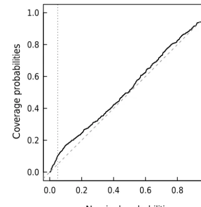
ex-Nominal probabilities Co ve ra ge p ro ba bi lit ie s

0.0 0.2 0.4 0.6 0.8 1.0

Figure 4.Coverage of one-sided bootstrapped prediction intervals (0,eqα(s)) for 528 ECEC validation samples plotted against nominal

probabilityαused to construct the upper limit qα of the prediction intervals (vertical lines mark the 5 and 95 % probabilities).

Table 3.Validation statistics for (a) log-transformed and (b) back-transformed ECEC 0–20 cm [mmolckg−1] calculated for 528 sam-ples (293 sites) of the independent validation set (for a definition of the statistics, see Sect. 3.3.3).

BIAS robBIAS RMSE robRMSE SSmse

(a) 0.052 0.006 0.471 0.411 0.407

(b) 6.3 8.9 74.9 55.3 0.365

plained about 40 % of the variance in the log-transformed and 37 % of the variance in the original data (Table 3).

Figure 4 shows somewhat too-large coverage for quantiles in the lower tails of the predictive distributions, and hence the extent of the lower tails of bootstrapped predictive distri-butions was underestimated. The upper tails of the predictive distributions were modelled accurately as the coverage was close to the nominal probability there. The coverage of sym-metric 90 % prediction intervals was again too small (84.1 %) because the lower tails were too short. The median width of 90 % prediction intervals was equal to 201.8 mmolckg−1,

demonstrating that prediction uncertainty remained substan-tial in spite of SSmseof nearly 40 %.

4.1.3 Mapping ECEC for ZH forest topsoils

(11)

soils are mostly found in the northern part of the Canton of Zurich. The spatial pattern of the width of 90 % predic-tion intervals (Fig. S3) and of the mean predicpredic-tions (Fig. 5) was very similar (Pearson correlation=0.981), which fol-lows from the log-normal model that we adopted for this re-sponse.

4.2 Presence of waterlogged soil horizons – case study 2

4.2.1 Models for the presence of waterlogged horizons

Not surprisingly, the models for thepresence of waterlogged horizonsin the three soil depths contained similar covariates characterising mostly wet soil conditions, such as historic wetland maps, a map of agricultural drainage systems or sev-eral climatic covariates (Table 2). The same terrain attributes were repeatedly chosen for the three depths (Figs. S4 to S6). For all three depths, model selection resulted in parsimonious sets of only 7 to 14 covariates chosen from a total of 498 co-variates. The Brier skill score (BSS), computed using 10-fold cross-validation, increased from 0.350 for the 0–30 cm depth to 0.704 for the 0–100 cm depth, suggesting that the pres-ence of waterlogged horizonscan be better modelled when is occurs more frequently. The degree of residual spatial auto-correlation on a logit scale was stronger in 0–30 cm than in 0–100 cm of depth (Fig. S2), confirming that the model per-formed better for the 0–100 cm depth. Adding thefs(s) term

did not improve cross-validated BSS (30 cm: 0.332, 100 cm: 0.688), meaning that a penalised tensor product of spatial co-ordinates was too smooth to capture short-range autocorrela-tion.

4.2.2 Validation of predicted presence of waterlogged horizons with independent data

Table 4 reports contingency tables for the predicted outcomes of thepresence of waterlogged horizonsat 198 sites of the validation set. BSS and the bias ratio improved again from the 0–30 cm to the 0–100 cm depth. In 0–30 cm of depth, the presence of waterlogged horizons was clear and down to 50 cm slightly over-predicted, while down to 100 cm there was no bias. The performance evaluated by percentage cor-rect with the Peirce skill score (PSS) was similar for all three depths (correct predictions being 44 to 50 % more frequent compared to random predictions). Ignoring correct absence

predictions in the Gilbert skill score (GSS), the model pre-dicted the correct level 20–30 % more often than a random prediction scheme. Again, GSS increased with depth and there was a higher chance of waterlogging occurring.

4.2.3 Mapping of the presence of waterlogged horizons

The presence of waterlogged horizons in 0–30 cm was pre-dicted for 13.8 % of the study region Greifensee (Fig. 6). For 0–50 cm this share increased to 27.3 % and in nearly

40 % of the soils waterlogged horizons were present in 0– 100 cm. Waterlogged horizons were mapped in upper soil depths mainly on the larger plains to the north and south of Greifensee. Deeper horizons had waterlogging present mostly in local depressions and comparably smaller valley bottoms in the hilly uplands to the south of the study region.

4.3 Drainage classes – case study 3 4.3.1 Model for drainage classes

The models for the ordinal drainage class data contained about the same covariates as the models for the presence of waterlogged horizons(Table 2). Most covariates had only very weak non-linear effects (Fig. S7). Residual spatial auto-correlation was very weak with a short range (Fig. S2), sug-gesting that the variation was well captured by the geoGAM. Then-fold cross-validation resulted in a ranked probability skill score (RPSS) of 0.588.

4.3.2 Validation of predicted drainage classes with independent data

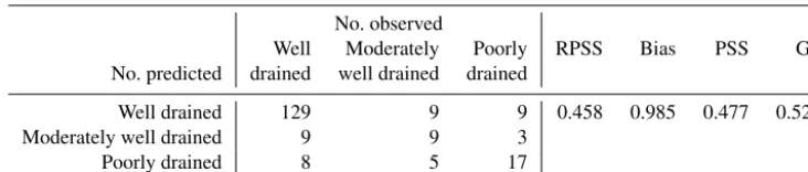
Table 5 reports the number of correctly classified and mis-classified drainage class predictions for the validation set. False predictions were equally distributed above and below the diagonal, and hence predictions were unbiased with a mean bias ratio close to 1. Distinguishing moderately well drainedsoils from the other two classes remained difficult as this class had been seldom observed. Overall, the model accuracy was satisfactory, with RPSS of 0.458 being only slightly smaller than cross-validation RPSS. Hence, the ge-oGAM was clearly better than always predicting the most abundant class,well drained. Measured by PSS and Gerrity score (GS), the geoGAM was better than random predictions at every second site for which predictions were computed.

4.3.3 Mapping of drainage classes

(12)

0 5 10 15 km

Data sources:

ECEC 0–20 cm [mmol kg ]_c -1

Validation sites (293) Calibration sites (1055)

Lake

< 25 25–50 51–100 101–200 201–300 301–500 > 500 Extremely small

Very small Small Medium

Large Very large Extremely large

Zurich

Winterthur

Uster

Uster

No forest

Figure 5.The geoGAM predictions of effective cation exchange capacity (ECEC) at 0–20 cm of depth in the mineral soil of forests in the Canton of Zurich, Switzerland (computed on a 20 m grid with final geoGAM with covariates according to Table 2. Black dots are locations used for geoGAM calibration, locations with red triangles were used for model validation and ECEC legend classes are according to Walthert et al., 2004).

Table 4.Observed occurrence of waterlogged horizons at three soil depths against predictions by geoGAM for the 198 sites of the validation set. Waterlogged soil horizons were predicted to be present if prediction probabilities were larger than an optimal threshold (30 cm: 0.22, 50 cm: 0.35, 100 cm: 0.51) found by cross-validation with Gilbert skill scores as criteria (No.: number of sites per response level, BSS: Brier skill score, bias: bias ratio, PSS: Peirce skill score, GSS: Gilbert skill score).

Waterlogged No. observed

BSS Bias PSS GSS

down to No. predicted Present Absent

30 cm Present 16 27 0.312 1.720 0.484 0.227

Absent 9 146

50 cm Present 28 25 0.448 1.152 0.444 0.267

Absent 18 127

100 cm Present 43 22 0.526 1.000 0.496 0.330

(13)

Table 5.Frequency of drainage class levels and predictions of respective outcomes by geoGAM for the 198 sites of the validation set (No.: number of sites per response level, RPSS: ranked probability skill score, bias: mean bias ratio, PSS: Peirce skill score, GS: Gerrity score for ordered responses).

No. observed

RPSS Bias PSS GS

Well Moderately Poorly No. predicted drained well drained drained

Well drained 129 9 9 0.458 0.985 0.477 0.523

Moderately well drained 9 9 3

Poorly drained 8 5 17

5 Discussion

5.1 Model building and covariate selection

The model-building procedure efficiently selected parsimo-nious models withp ≤17 covariates for all responses. This corresponds to only 5.8 % of the covariates considered for the effective cation exchange capacity (ECEC) modelling and to 1.4–2.8 % for modelling the binary and ordinal responses de-scribing waterlogging.

The procedure was able to select meaningful covariates, which reveal the influence of soil-forming factors on the re-sponse variable, without any prior knowledge about the im-portance of a particular covariate. No preprocessing of co-variates was necessary, e.g. reducing the dimensionality of the covariate set to deal with multi-collinearity. This is es-pecially important for terrain covariates. Elevation data are often available in several resolutions, and various algorithms can be used to calculate curvature or topographic wetness in-dices (TWI), which all likely produce slightly different re-sults. In addition, radii for computing, for example, topo-graphic position indices (TPI) have to be specified, and it is often not a priori clear how these should be chosen (Behrens et al., 2010; Miller et al., 2015). Therefore, different algo-rithms and a range of parameter values are used to create terrain covariates, and the model-building process selects the most suitable covariate to model a particular soil property. Meanwhile, none of the 180 APEX bands available for the Greifensee region were chosen for the final models. Most likely, meaningful preprocessing, for example based on bare soil areas, could improve the usefulness of such covariates (Diek et al., 2016). Since we used continuous reflectance sig-nals, including vegetated and sparsely vegetated areas, the remotely sensed signal might not have expressed direct rela-tionships to actual soil properties well.

5.2 Model structure

Parsimonious models lend themselves to a verification of fit-ted effects from a pedological perspective. Yet, due to multi-collinearities in the covariate set, the effects of selected co-variates could be substituted by the effects of other coco-variates (Behrens et al., 2014).

Although Johnson et al. (2000) did not find strong rela-tionships between terrain and ECEC, six terrain attributes were selected. Covariates representing geology were impor-tant, too, with ECEC changing, for example, as a function of the distance to two types of moraines. Also, vegetation provided information on ECEC in the topsoil because a veg-etation index (difference of near infrared to red reflectance) and a vegetation map were included. Larger values of ECEC were modelled for plant communities that are characteris-tic of nutrient-rich soils. The factor distinguishing the origin of soil data either from direct measurement or pedotransfer function (PTF; legacy data correction; Sect. 3.2.2, Fig. S1) was further relevant in the ECEC model.

For modelling drainage classes and thepresence of water-logged horizons, plausible covariates were selected (Figs. S4 to S7). Most covariates were terrain attributes derived from the digital elevation model (DEM). This is in accordance with Campling et al. (2002), who found topography impor-tant in general, and Lemercier et al. (2012), who showed that a topographic wetness index was among the most important covariates. Local depression at various scales (concave cur-vature, basins in TPI, sites with accumulation by erosion, terrain wetness) increased the probability ofpoorly drained

soils and thepresence of waterlogged horizons. More vari-able terrain (standard deviation of elevation) also increased waterlogging probability. Climate covariates also seemed to be important. The rainfall pattern in summer (June, July), the spring dew point temperature and global radiation (March, April) correlated most strongly with thepresence of water-logged horizons. Information on human activities related to waterlogged soil amelioration was included in all four mod-els. Maps of historic wetlands and areas with drainage sys-tems were most often chosen in combination. Geology was also partly relevant (thepresence of waterlogged horizonsin 0–100 cm of soil depth and drainage classes).

(14)

re-0 5 10 km Calibration

Validation

Waterlogged

Absent Present

Lake

Data sources:

(c) Soil depth: 0–100 cm (b) Soil depth: 0–50 cm

(a) Soil depth: 0–30 cm

sites (764)

sites (198) Zurich

Zurich

soil horizon

Figure 6.The geoGAM predictions of the presence of waterlogged horizons between the surface and three soil depths ((a)0–30,(b)0– 50,(c)0–100 cm) for the agricultural land in the Greifensee study region (computed on a 20 m grid with final geoGAM, with covari-ates according to Table 2, smoothed for better display with focal mean with radius of 3 pixels=60 m). Black dots in panel(a)are locations used for geoGAM calibration, and locations with red tri-angles were used for model validation.

0 5 10 km

Zurich

Calibration sites (732) Validation sites (198)

Drainage class Well drained

well drained Moderately

drained Poorly Lake

Data sources:

Greifensee

Lake of

Zuri ch

2013 FABO Canton of Zurich (TID 22742)

Figure 7.The geoGAM predictions of drainage classes for the agricultural land in the Greifensee study region (computed on a 20 m grid with final geoGAM, with covariates according to Table 2, smoothed for better display with focal mean with radius of 3 pix-els=60 m). Black dots are locations used for geoGAM calibration, and locations with red triangles were used for model validation.

gion and the response being a chemical property that depends on various combinations of soil-forming factors evidently re-quired the use of a more complex model.

5.3 Predictive performance of fitted models

For the final models, cross-validation statistics were similar to the results obtained for the independent validation data. Through repeated cross-validation on the same subsets, the cross-validation statistics can be considered as conservative goodness-of-fit statistics. Hence, we conclude that geoGAM did not over-fit the calibration data.

Independently validated model accuracy was satisfactory for ECEC in the present study with (SSmse 0.37). Compared

to the few available studies, the quality of our maps of ECEC was intermediate. Building a separate model for forest soil ECEC for a dataset with about 2.1 sites per km2seem to pro-duce much better results than the study reported by Vaysse and Lagacherie (2015), who found very poor model perfor-mance for ECEC (R2=0, equivalently computed as SSmse)

(15)

Viscarra Rossel et al. (2015, Supplement) reportedR2of 0.79 (computed as SSmse) for topsoil ECEC for Australia. In the

studies of Hengl et al. and Viscarra Rossel et al., ECEC var-ied much more than in our study, and this likely explains the better quality of the predictions.

Our models for the presence of wet soils reached similar accuracy as reported in other studies. Zhao et al. (2013, Ta-ble 1) reported that 64 to 87 % of the sites were correctly classified (percentage correct, PC) in four studies that mod-elled three drainage class levels. Three studies with up to seven drainage levels achieved PC of 52 to 78 %, and Zhao et al. (2013) had 36 % of correctly classified sites. Kidd et al. (2014) found PC of 53 and 55 % for two study regions, and Lemercier et al. (2012) reported PC of 52 % for a four-level drainage response. The presented models (Table 4 and 5) are almost as good with PC of 78 to 82 % for predicting the pres-ence of waterlogged horizonsand PC of 78 % for predicting the three drainage class levels.

Nevertheless, PC is trivial to hedge (Jolliffe and Stephen-son, 2012, pp. 46), and comparisons should be made only with care. Better performance measures are PSS and Cohen’s kappa (κ), also called the Heidke skill score (Wilks, 2011, pp. 347). Campling et al. (2002) reported aκof 0.705, Kidd et al. (2014) found κ values of 0.27 and 0.31 for the two study regions, Lemercier et al. (2012) reported aκ of 0.27 and Peng et al. (2003) found a κ of 0.59 for predictions of three drainage levels. Theκ values computed for the models of this study ranged between 0.37 and 0.5 for modelling the

presence of waterlogged horizonsand was 0.48 for predict-ing the three levels of drainage class. Unequal distributions of the three drainage classes in the study region (the major-ity of soils werewell drained) were reflected in the smaller value ofκ compared to PC.

5.4 Spatial structure of predicted maps

The spatial distribution of ECEC as shown by Fig. 5 aligns well with pedological knowledge about soils in the Can-ton of Zurich. The smallest ECEC (<50 mmolckg−1) was

mapped in the north-east of the study region. The last glacia-tion (Swisstopo, 2009) did not reach as far north and, as a consequence, strongly weathered soils on old fluvioglacial gravel-rich sediments developed in this part of the study re-gion. Soils not covered by ice during the last glaciation have comparably larger ECEC if they formed on Molasse.

As expected, the spatial patterns for the presence of wa-terlogged soil horizons and the drainage classes were very similar (Fig. 6 and 7). Soils on plains to the north and south of Greifensee are oftenpoorly drained, although at many lo-cations agricultural drainage networks were installed in the past.

6 Summary and conclusion

Effectively building predictive models for digital soil map-ping (DSM) becomes crucial if many soil properties are to be mapped. Selecting only a small set of relevant covariates ren-ders interpretation of the fitted models easier and allows for a check of whether modelled relations accord with pedologi-cal understanding. Parsimonious, interpretable DSM models are likely more readily accepted by end-users than complex black-box models. Moreover, model selection out of a large number of covariates describing soil-forming factors helps to improve knowledge about relationships at larger scales. In this sense, it is also important that the modelling approach provides information about covariates which are not rele-vant for a certain response, e.g. the large number of APEX bands for thepresence of waterlogged horizonsand drainage classes.

We developed a model-building framework for generalised additive models for spatial data (geoGAM) and applied the framework to legacy soil data from the Canton of Zurich (Switzerland). We found that geoGAM did the following:

– consistently modelled continuous, binary and ordinal responses, hence allowing for the DSM of measured soil properties and soil classification data using one com-mon approach;

– selected, given the large numbers of covariates, ade-quately small sets of pedogenetically meaningful co-variates without any prior knowledge about their impor-tance and without prior reduction of the covariate sets;

– required minimal user interaction for model building, which facilitates future map updates as new soil data or new covariates become available;

– allowed for easy interpretation of the effects of the in-cluded covariates with partial residual plots;

– modelled predictive distributions for continuous re-sponses with a bootstrapping approach, thereby taking the uncertainty of model building into account,

– did not over-fit the calibration data in our applications; and

– predicted soil properties with similar accuracy as other approaches in other digital soil mapping studies when tested with an independent validation set.

(16)

Code availability. The geoGAM model-building procedure was published as R packagegeoGAM(Nussbaum, 2017).

Data availability. The soil data were used under a nonpublic data licence (Canton of Zurich, contract number TID 22742; WSL) and could not be published.

The Supplement related to this article is available online at https://doi.org/10.5194/soil-3-191-2017-supplement.

Author contributions. AP proposed the application of component-wise gradient boosting with smooth base learners for DSM. MN implemented the framework and adapted it to the needs of DSM. LW harmonised the soil data with collaborators, and MF computed multi-scale terrain attributes. LG defined the responses for the presence of waterlogged soil horizons and drainage classesfrom Swiss soil classification data. MN prepared the paper with major input from AP and further contributions from all co-authors.

Competing interests. The authors declare that they have no con-flict of interest.

Acknowledgements. We thank the Swiss National Science Foundation SNSF for funding this work in the framework of the na-tional research programme “Sustainable Use of Soil as a Resource” (NRP 68). We also thank the Swiss Earth Observatory Network (SEON) for funding aerial surveys with APEX. Special thanks go to WSL and the soil protection agency of the Canton of Zurich for sharing their soil data with us. Furthermore, we would like to thank Thorsten Hothorn for advice on model selection and boosting.

Edited by: Bas van Wesemael Reviewed by: two anonymous referees

References

Adhikari, K., Kheir, R., Greve, M., Bøcher, P., Malone, B., Minasny, B., McBratney, A., and Greve, M.: High-resolution 3-D mapping of soil texture in Denmark, Soil Sci. Soc. Am. J., 77, 860–876, https://doi.org/10.2136/sssaj2012.0275, 2013.

ALN: Historische Feuchtgebiete der Wildkarte 1850. Amt für Landschaft und Natur des Kantons Zürich, available at: http://www.aln.zh.ch/internet/baudirektion/aln/de/naturschutz/ naturschutzdaten/geodaten.html (last access: 29 March 2017), 2002.

ALN: Geologische Karte des Kantons Zürich nach Hantke et al. 1967, GIS-ZH Nr. 41. Amt für Landschaft und Natur des Kan-tons Zürich, available at: http://www.gis.zh.ch/Dokus/Geolion/ gds_41.pdf (last access: 15 February 2015), 2014a.

ALN: Meliorationskataster des Kantons Zürich, GIS-ZH Nr. 148. Amt für Landschaft und Natur des Kantons Zürich, available at: http://www.geolion.zh.ch/geodatensatz/show?nbid=387 (last ac-cess: 29 March 2017), 2014b.

AWEL: Hinweisflächen für anthropogene Böden, GIS-ZH Nr. 260. Amt für Abfall, Wasser, Energie und Luft des Kanton Zürich, available at: http://www.geolion.zh.ch/geodatensatz/show?nbid= 985 (last access: 29 March 2017), 2012.

AWEL: Grundwasservorkommen, GIS-ZH Nr. 327. Amt für Ab-fall, Wasser, Energie und Luft des Kanton Zürich, available at: http://www.geolion.zh.ch/geodatensatz/show?nbid=723 (last ac-cess: 29 March 2017), 2014.

AWEL: NO2-Immissionen, GIS-ZH Nr. 82, Amt für Abfall, Wasser, Energie und Luft des Kanton Zürich, available at: http://geolion.zh.ch/geodatensatz/show?nbid=783 (last access: 29 March 2017), 2015.

BAFU: Luftbelastung: Karten Jahreswerte, Ammoniak und Stickstoffdeposition, Jahresmittel 2007 (modelliert durch METEOTEST), available at: http://www.bafu.admin.ch/luft/ luftbelas-tung/schadstoffkarten (last access: 15 February 2015), 2011.

Behrens, T., Schmidt, K., Zhu, A. X., and Scholten, T.: The ConMap approach for terrain-based digital soil mapping, Eur. J. Soil. Sci., 61, 133–143, https://doi.org/10.1111/j.1365-2389.2009.01205.x, 2010.

Behrens, T., Schmidt, K., Ramirez-Lopez, L., Gallant, J., Zhu, A.-X., and Scholten, T.: Hyper-scale digital soil map-ping and soil formation analysis, Geoderma, 213, 578–588, https://doi.org/10.1016/j.geoderma.2013.07.031, 2014.

Ben-Dor, E., Chabrillat, S., Demattê, J. A. M., Taylor, G. R., Hill, J., Whiting, M. L., and Sommer, S.: Using imaging spectroscopy to study soil properties, Remote Sens. Environ., 113, S38–S55, https://doi.org/10.1016/j.rse.2008.09.019, 2009.

BFS: GEOSTAT Benützerhandbuch, Bundesamt für Statistik, Bern, 2001.

Bourennane, H., King, D., Chéry, P., and Bruand, A.: Improving the kriging of a soil variable using slope gradient as external drift, Eur. J. Soil. Sci., 47, 473–483, https://doi.org/10.1111/j.1365-2389.1996.tb01847.x, 1996.

Brassel, P. and Lischke, H. (Eds.): Swiss National Forest Inventory: Methods and models of the second assessment, Swiss Federal Institute for Forest, Snow and Landscape Research WSL, Bir-mensdorf, 2001.

Breheny, P. and Huang, J.: Group descent algorithms for nonconvex penalized linear and logistic regression mod-els with grouped predictors, Stat Comput, 25, 173–187, https://doi.org/10.1007/s11222-013-9424-2, 2015.

Brunner, J., Jäggli, F., Nievergelt, J., and Peyer, K.: Kartieren und Beurteilen von Landwirtschaftsböden, FAL Schriftenreihe 24, Eidgenössische Forschungsanstalt für Agrarökologie und Land-bau, Zürich-Reckenholz (FAL), 1997.

Buchanan, S., Triantafilis, J., Odeh, I. O. A., and Subansinghe, R.: Digital soil mapping of compositional particle-size frac-tions using proximal and remotely sensed ancillary data, Geo-physics, 77, WB201–WB211, https://doi.org/10.1190/geo2012-0053.1, 2012.

(17)

Campling, P., Gobin, A., and Feyen, J.: Logistic mod-eling to spatially predict the probability of soil drainage classes, Soil Sci. Soc. Am. J., 66, 1390–1401, https://doi.org/10.2136/sssaj2002.1390, 2002.

Cleveland, W. S.: Robust Locally Weighted Regression and Smoothing Scatterplots, J. Am. Stat. Assoc., 74, 829–836, https://doi.org/10.2307/2286407, 1979.

Conrad, O., Bechtel, B., Bock, M., Dietrich, H., Fischer, E., Gerlitz, L., Wehberg, J., Wichmann, V., and Böhner, J.: System for Auto-mated Geoscientific Analyses (SAGA) v. 2.1.4, Geosci. Model Dev., 8, 1991–2007, https://doi.org/10.5194/gmd-8-1991-2015, 2015.

Cressie, N.: Block Kriging for Lognormal Spatial Processes, Math. Geol., 38, 413–443, https://doi.org/10.1007/s11004-005-9022-8, 2006.

Danner, C., Hensold, C., Blum, P., Weidenhammer, S., Aussendorf, M., Kraft, M., Weidenbacher, A., Holleis, P., and Kölling, C.: Das Schutzgut Boden in der Planung, Bewertung natürlicher Bodenfunktionen und Umsetzung in Planungs-und Genehmigungsverfahren, Bayerisches Landesamt für Umweltschutz, Bayerisches Geologisches Landesamt, avail-able at: http://www.lfu.bayern.de/boden/bodenfunktionen/ ertragsfaehigkeit/doc/arbeitshilfe_boden.pdf (last access: 29 March 2017), 2003.

Davison, A. C. and Hinkley, D. V.: Bootstrap Methods and Their Applications, Cambridge University Press, Cambridge, https://doi.org/10.1017/cbo9780511802843, 1997.

de Brogniez, D., Ballabio, C., Stevens, A., Jones, R. J. A., Montanarella, L., and van Wesemael, B.: A map of the topsoil organic carbon content of Europe generated by a generalized additive model, Eur. J. Soil Sci., 66, 121–134, https://doi.org/10.1111/ejss.12193, 2015.

Diek, S., Schaepman, M., and de Jong, R.: Creating multi-temporal composites of airborne imaging spectroscopy data in support of digital soil mapping, Remote Sens., 8, 906, https://doi.org/10.3390/rs8110906, 2016.

Dirichlet, G. L.: Über die Reduction der posi-tiven quadratischen Formen mit drei unbestimmten ganzen Zahlen, J. reine angew. Math., 40, 209–227, https://doi.org/10.1017/cbo9781139237345.005, available at: http://eudml.org/doc/147457, 1850.

DMC: Disaster Monitoring Constellation International Imaging, available at: http://www.dmcii.com, last access: 3 February 2015. Dobson, A. J.: An Introduction to GeneralIzed Linear Models,

Chapman & Hall/CRC, Boca Raton, 2002.

ELF: Schweizerische Referenzmethoden der Forschungsanstalten Agroscope – Boden- und Substratuntersuchungen zur Düngeber-atung, Loseblattordner E1.011.d 1, Forschungsanstalten Agro-scope ART und ACW, Zürich und Changins, Ausgabe 1996 mit Änderungen von 1997 bis 2009, Version 2015, Methode “AAE-10”, 1996.

ESRI: ArcGIS Desktop: Release 10, ESRI Environmental Sys-tems Research Institute, Redlands, California, USA., available at: www.esri.com (last access: 29 March 2017), 2010.

FAC: Methoden für Bodenuntersuchungen, no. 5 in Schriften-reihe der FAC, Liebefeld, Eidgenössische Forschungsanstalt für Agrikulturchemie und Umwelthygiene (FAC), 1989.

FAO and ITPS: Status of the World’s Soil Resources (SWSR), Main report, Food and Agriculture Organization of the United Nations

and Intergovernmental Technical Panel on Soils, Rome, Italy, 2015.

Faraway, J. J.: Linear Models with R, vol. 63 of: Texts in Statistical Science, Chapman & Hall/CRC, Boca Raton, 2005.

Fitzpatrick, B. R., Lamb, D. W., and Mengersen, K.: Ultrahigh Di-mensional Variable Selection for Interpolation of Point Refer-enced Spatial Data: A Digital Soil Mapping Case Study, PLoS One, 11, 1–19, https://doi.org/10.1371/journal.pone.0162489, 2016.

Frigge, M., Hoaglin, D. C., and Iglewicz, B.: Some implemen-tations of the boxplot, The American Statistician, 43, 50–54, https://doi.org/10.2307/2685173, 1989.

FSO: Swiss soil suitability map. BFS GEOSTAT. Swiss Federal Sta-tistical Office, available at: http://www.bfs.admin.ch/bfs/portal/ de/index/dienstleistungen/geostat/datenbeschreibung/digitale_ bodeneignungskarte.html (last access: 15 February 2015), 2000a.

FSO: Tree composition of Swiss forests. BFS GEO-STAT. Swiss Federal Statistical Office, available at: http://www.bfs.admin.ch/bfs/portal/de/index/dienstleistungen/ geostat/datenbeschreibung/waldmischungsgrad.html (last access: 15 February 2015), 2000b.

Gasser, U., Gubler, A., Hincapié, I., Karagiannis, D.-A., Schwierz, C., and Zimmermann, S.: Bestimmung der Austauschereigen-schaften von Waldböden: Kostenoptimierung, Bulletin Bo-denkundliche Gesellschaft der Schweiz, 32, 51–52, 2011. Grimm, R., Behrens, T., Märker, M., and Elsenbeer, H.: Soil organic

carbon concentrations and stocks on Barro Colorado Island – Digital soil mapping using Random Forests analysis, Geoderma, 146, 102–113, https://doi.org/10.1016/j.geoderma.2008.05.008, 2008.

Hantke, R. U.: Geologische Karte des Kantons Zürich und seiner Nachbargebiete, Kommissionsverlag Leemann, Zürich, Sonder-druck aus: Vierteljahrsschrift der Naturforschenden Gesellschaft in Zürich, 112: 91–122, 1967.

Hastie, T. J. and Tibshirani, R. J.: Generalized Additive Models, vol. 43 of: Monographs on Statistics and Applied Probability, Chapman and Hall, London, 1990.

Hastie, T., Tibshirani, R., and Friedman, J.: The Elements of Statis-tical Learning; Data Mining, Inference and Prediction, Springer, New York, 2 edn., 2009.

Henderson, B. L., Bui, E. N., Moran, C. J., and Simon, D. A. P.: Australia-wide predictions of soil proper-ties using decision trees, Geoderma, 124, 383–398, https://doi.org/10.1016/j.geoderma.2004.06.007, 2005.

Hengl, T., de Jesus, J. M., MacMillan, R. A., Bat-jes, N. H., Heuvelink, G. B. M., Ribeiro, E., and Samuel-Rosa, A.: SoilGrids1km – Global Soil Infor-mation Based on Automated Mapping, PLoS One, 9, https://doi.org/10.1371/journal.pone.0105992, 2014.