www.ocean-sci.net/4/1/2008/
© Author(s) 2008. This work is licensed under a Creative Commons License.
Ocean Science
A high-resolution free-surface model of the Mediterranean Sea
M. Tonani1, N. Pinardi2, S. Dobricic3, I. Pujol1, and C. Fratianni1
1Istituto Nazionale di Geofisica e Vulcanologia, Bologna, Italy 2University of Bologna, Corso di Scienze Ambientali, Ravenna, Italy 3Centro Euro-Mediterraneo per i Cambiamenti Climatici, Bologna, Italy Received: 8 January 2007 – Published in Ocean Sci. Discuss.: 26 February 2007
Revised: 16 November 2007 – Accepted: 13 December 2007 – Published: 24 January 2008
Abstract. This study describes a new model implementation
for the Mediterranean Sea with what is currently the highest vertical resolution over the Mediterranean basin. The resolu-tion is of 1/16◦×1/16◦in the horizontal and has 72 unevenly spaced vertical levels. This model has been developed in the frame of the EU-MFSTEP project and is the operational fore-cast model currently used at the basin scale.
The model considers an implicit free surface and this char-acteristic enhances the model’s capability to simulate the sea surface height variability and the net transport at the Strait of Gibraltar.
In this study we show the calibration/validation experi-ments performed before and after the model was used for forecasting. The first experiment consists of a six-year simu-lation forced by a perpetual year forcing, and the other exper-iment is a simulation from January 1997 to December 2004, forcing the model with 6-h atmospheric forcing fields from ECMWF. The model Sea Level Anomaly has been compared for the first time with satellite SLA and with ARGO data to provide evidence of the quality of the simulation.
The results show that this model is capable of reproduc-ing most of the variability of the general circulation in the Mediterranean Sea. However, some basic model inadequa-cies stand out and should be corrected in the near future.
1 Introduction
The aim of this study is to give a detailed description of the Mediterranean Sea forecasting model implementation stud-ies performed during the MFSTEP project in order to assess the quality of the numerical model that is now used for the daily forecasts at the basin scales.
Correspondence to: M. Tonani (tonani@bo.ingv.it)
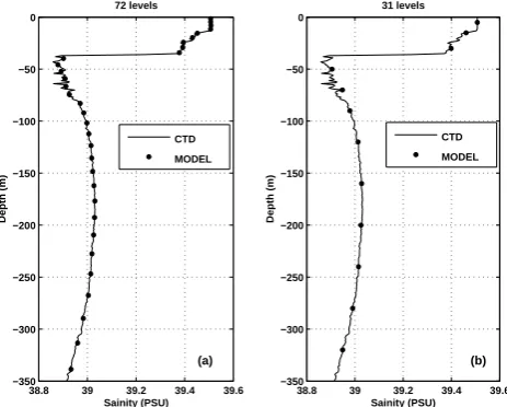
38.8 39 39.2 39.4 39.6 −350 −300 −250 −200 −150 −100 −50 0 Depth (m) Sainity (PSU) 72 levels (a) CTD MODEL
38.8 39 39.2 39.4 39.6 −350 −300 −250 −200 −150 −100 −50 0 Depth (m) Sainity (PSU) 31 levels (b) CTD MODEL
Fig. 1. Salinity profile from CTD in the eastern Mediterranean and
its discretisazion by the model levels for the case of 72 levels (panel
a) and 31 levels (panel b). The full line is the CTD profiles and the
dots represents the depths of the model vertical levels.
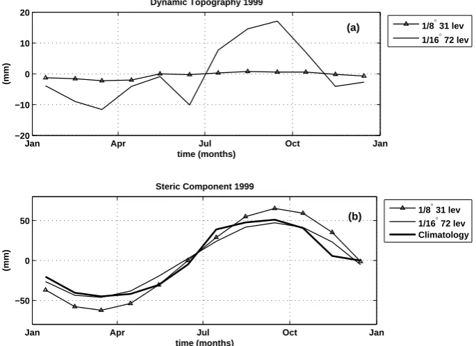
in fact have a net transport at Gibraltar, and this is a fea-ture missing from all previous high-resolution simulations. Figure 2 shows a comparison between the dynamic topog-raphy (panel a) and the steric component (panel b) between the rigid lid 1/8◦×1/8◦horizontal resolution model and the free-surface 1/16◦×1/16◦model. The comparison was made for 1999. The low-resolution rigid lid model is not able to simulate the seasonal variability of the dynamic topography well, and has a really smooth shape with respect to the free-surface and high-resolution model. The dynamic topography has been computed from the sea surface pressure for the rigid lid model and from the sea surface high for the free-surface one. Panel b) shows the variability of the sea level high due to the steric effect. We have computed this variabillity from the climatological data of MEDATLAS (MEDAR/MEDATLAS Group 2002) and from the two model simulations. It is clear from Fig. 2 that the low resolution model has a higher vari-ability, which could be due to the low vertical resolution of the model that is not adequate to represent the seasonal vari-ability of the characteristics of the water column. The high-resolution model, on the contrary, has a variability much closer to the steric component of the climatology; it there-fore seems to be more efficient in the simulation of the water column property variability due to the seasonal variability.
This paper is organized in the following way: Sect. 2 gives a detailed description of the model equations and parameter choices; Sect. 3 describes the experimental design; Sect. 4 describes the simulation results and the comparison with the observations; Sect. 5 offers the conclusions.
2 Model equations and parameter choices
2.1 Model equations and domain of implementation The model uses the primitive equations with the Boussinesq and incompressible approximations written in spherical co-ordinates(λ, ϕ, z), whereϕ is the latitude,λthe longitude andzthe depth. The set analytical expressions for the equa-tions are:
∂u
∂t =(ζ+f ) v−w
∂u
∂z−
1 2acosϕ
∂ ∂λ
u2+v2
− 1
ρ0acosϕ
∂p
∂λ −A
lm∇4u+ ∂
∂z
Avm∂u
∂z
(1)
∂v
∂t = −(ζ+f ) u−w
∂v ∂z− 1 2a ∂ ∂ϕ
u2+v2
− 1
ρ0a
∂p
∂ϕ −A
lm∇4v+ ∂
∂z
Avm∂v
∂z
(2)
∂p
∂z = −ρg (3)
1
αcosϕ
∂u
∂λ+
∂
∂ϕ[cosϕv]
+∂w
∂z =0 (4)
∂θ
∂t = −
1
acosϕ
∂
∂λ(θ u)+
∂
∂ϕ(cosϕθ v)
− ∂
∂z(θ w)
−AlT∇4T +AvT∂
2θ
∂z2 +δµ θ
∗−
θ
(5)
∂S
∂t = −
1
αcosϕ
∂
∂λ(Su)+
∂
∂ϕ(cosϕSv)
− ∂
∂z(Sw)
−A1S54S+AvS∂
2S
∂z2 +δµ(S
∗−
S) (6)
ρ=ρ(T , S, p) (7)
where we recognize that the momentum equations have been re-written in their vorticity form (Pedlosky 1983). In Eqs. (1) to (7), u, v, w are the components of the velocity vector;
ς= 1
acosϕ
∂v ∂λ−
∂
∂ϕ[ucosϕ]
is the vorticity;a the earth ra-dius; f=2sinϕ the Coriolis term with the constant earth rotation rate;p the hydrostatic pressure; θ the poten-tial temperature, S the salinity, ρ the in situ density and
ρo=1020 kg/m3 the reference density; Alm, Avm the
hor-izontal and vertical eddy viscosities; AvT, AvS the vertical diffusivities;AlT, AlSthe horizontal diffusivities;δandµare the relaxation coefficients, which will be described in details later.
Jan Apr Jul Oct Jan −20
−10 0 10 20
time (months)
(mm)
Dynamic Topography 1999
(a) 1/8° 31 lev 1/16° 72 lev
Jan Apr Jul Oct Jan
−50 0 50
time (months)
(mm)
Steric Component 1999
(b) 1/8
° 31 lev
1/16° 72 lev Climatology
Fig. 2. comparison between the rigid lid low resolution model and the free-surface high-resolution one. Panel (a) shows the mean dynamic
topography (mm) for 1999 computed from the two models respectively as sea surface high or pressure minus the mean over all of 1999. The line with triangles is the dynamic topography from the low-resolution model whilst the continuous line is the high-resolution model. The values are computed as monthly means and are mean over the whole Mediterranean basin. Panel (b) show the comparison of the steric component (mm) computed from the temperature and salinity fields of the two models (line with triangles for the low-resolution model) and from the monthly mean climatology MEDATLAS (thick line).
variable. The numerical scheme for the free surface is de-scribed by Roullet et al. (2000).
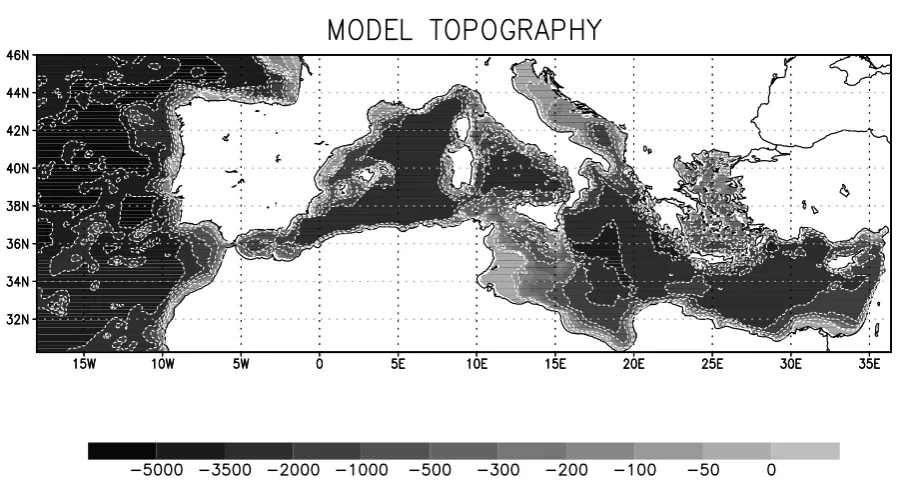
The model domain and the bathymetry are shown in Fig. 3: the coastline resolves 49 islands. The procedure used to make the coastline, the bathymetry and the vertical level distribution is described in the Appendix. The Atlantic box is very large with respect to previous implementations (Demirov and Pinardi, 2002) and it will be described in de-tail below.
2.2 Sub-grid-scale parameterizations
The horizontal eddy viscosity (Alm)is considered to be a constant value of 5×10⁹m4/s whilst the horizontal diffusiv-ities (AlT, AlS)are equal and set to the value of 3×10⁹m4/s. The vertical diffusivities (AvS, AvT)and viscosity (Avm)are a function of the Richardson number as parametrized by Pakanowsky and Philander-PP (1981), i.e.:
AvT = 100×10
−4
(1+5(N2/(∂U
h/∂z)2))2
+(1.5×10⁻⁴) (8)
Avm= A
vT
1+5(N2/(∂U
h/∂z)2)
+(3×10⁻⁴) (9) where the vertical salinity diffusivity is equal to Eq. (8). The PP parameterization is thought to be relevant for mixed-layer
processes whilst deep convection needs another parametriza-tion. The model thus uses enhanced vertical diffusion to produce deep convection: the vertical diffusivity and viscos-ity coefficients are assigned to be equal to 1 m2/s in regions where the stratification is unstable.
2.3 Vertical boundary conditions At the bottom,z=−H (x, y), we impose:
a) for the vertical velocity:
w= −ubh· 5H (10)
whereubh=(ub, vb)is the bottom velocity assumed to
be the deepest layer velocity;
b) for the momentum, temperature and salt flux:
Avm ∂
∂z(uh)|z=−H =CD
q
u2b+v2b+ebubh (11)
AvT ∂
∂z(T , S)|z=−H =0 (12)
whereCD=10−3 is the drag coefficient and eb is the
Fig. 3. Model bathymetry and domain.
waves breaking, and to all the other contributions at very short spatial and temporal scales.
At the surface,z=η, the boundary conditions are: a) for the vertical velocity
w= Dη
Dt −(E−P ) (13)
where DηDt=∂η
∂t+uh · ∇η P is the precipitation and E
the evaporation (E). This is the so-called water flux boundary condition.
b) The momentum boundary condition is:
Avm∂uh
∂z |z=n=
(τu, τv)
ρ0
(14) whereτu, τv are the zonal and meridional wind stress
components respectively.
c) The heat flux boundary condition is:
AvT∂T
∂z |z=0=
Q
ρ0Cp
(15)
whereCp=4000 J/(kg◦K) andQ (W/m2) is the
non-penetrative net heat flux at the surface. In our case, all the heat is assumed to be absorbed at the surface. d) The boundary condition for the salinity is:
ρ0AvS
∂S
∂z |z=0=(E−P )Sρ0 (16)
whereSis the surface salinity which corresponds to the water flux condition, Eq. (13).
The water flux has been chosen as:
ρ0(E−P )=γ−1
(S−S∗)
S (17)
whereSis the model surface salinity,S∗is the climato-logical surface salinity andγ=−0.007(m2s/kg)is the salinity relaxation coefficient. The corresponding relax-ation time is:
1
ρ0
γ−1(S−S
∗
S =
1z
1t
1t=ρ01zγ
S
S−S∗
(18)
If1z=3 m is the first model layer depth,1t∼=5 days. 2.4 The Atlantic box and the Strait of Gibraltar
southward boundaries and 3◦ at the northern boundary (in order to cover all the area of the Gulf of Biscay).
The µ coefficient varies spatially, whilst δ is a time factor: µ is larger closer to the boundary points of the box and linearly decreases to zero outside the strip and
δ=2.3×10⁻⁷ s−1. The horizontal diffusivities are also in-cremented by a factor of 5 in the Atlantic box strip areas in order to add a sponge layer.
Some modifications are necessary at the Strait of Gibral-tar to avoid unrealistic values of the transport at this strait. The horizontal viscosity is laplacian in the region between 6.25◦W and 5.125◦W, whilst in the rest of the basin it is bi-laplacian. The diffusivity in this area is 10 times larger than in the rest of the model. In the same geographical area the bottom friction drag coefficient is linear and ten times larger then in the other parts of the model. Out of the Strait of Gibraltar in the Atlantic Box, the bathymetry has been mod-ified in order to resolve the Camarinam Sill (Sannino et al., 2004).
2.5 The water flux correction
The domain of Fig. 3 has closed boundaries and care should be taken in considering the effects of net sources/sinks of heat and water in the basin. In the Atlantic box, heat and salt is added or substracted by the relaxation terms in Eqs. (5) and (6), which are different from zero along the strip of the lateral boundaries, as described above. These terms will balance the heat loss and the salt gain from the sea surface, over the Mediterranean part of the basin in particular.
However, care should be taken for the surface water boundary condition – Eq. (13) – which sets the sea surface height of the basin and therefore the mass conservation. We develop here a way to correct the water balance in a closed model domain that conserves mass under the conditions of negative surface net water flux. It is well known that the Mediterranean basin on a yearly average has a net water loss due toE exceedingP. The water lost at the surface of the Mediterranean Sea is balanced by a net inflow of water at the Gibraltar Strait. We need to enforce this balance so that the model volume does not drift.
The basin mean (E-P) is then separated into two compo-nents, the Atlantic and Mediterranean:
E−P =(E−P )MED+(E−P )ATL (19)
At each time step, the space integral of the Mediterranean and Atlantic water flux is computed and the sum of this two components of the water flux,1E−P,is computed:
Z
x,y
(E−P )MED+
Z
x,y
(E−P )ATL=1E−P (20)
1E−P will be now used to compute a new value for the
wa-ter flux over the Atlantic in order to have the net wawa-ter flux equal zero over the whole domain. This does not change the Mediterranean basin water loss, but it balances it so that
yr1 yr2 yr3 yr4 0
0.005 0.01 0.015 0.02 0.025
Δ
(E−P) (%)
TIME (years)
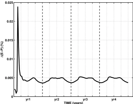
Fig. 4. Water flux correction factor,1(E−P ), over all the Atlantic box computed for the first five years of the perpetual year simula-tion. The value of1(E−P )is computed as the percentage of the total water flux value in the Atlantic Box.
mass is conserved. A value of(E−P )ATL CORRis therefore recomputed for each Atlantic grid point in the following way:
(E−P )ATL CORR=1E−P/AREAATL−(E−P )ATL (21) where AREAATLis the Atlantic surface area. This assump-tion can be made only if the model is not used for climate simulations that cover hundreds of years, a period over which the modification of the water flux into the Atlantic box may be relevant and non-negligible. Figure 4 shows the value of
1E−P computed as percentage of the(E−P )ATL CORR in one of the experiments studied in this paper. This value af-ter the first months of simulation decreases and assumes a value of ca. 0.005%. This value is small enough, and more-over does not increase during the simulation. Therefore we argue that this approximation,is valid for short term forecast-ing purposes.
2.6 Design of the numerical experiments
The model described in Sect. 2 was run with two different approximations of the atmospheric forcing:
1) the so-called perpetual year forcing, where the water, heat and momentum surface fluxes are monthly varying climatological mean values;
2) with 6-h meteorological forcing for the period January 1997 to December 2004.
1997 1998 1999 2000 2001 2002 2003 2004 2005 2
4 6 8 10 12 14
TIME (Years)
KE (m
2 /s 2 X 10 − 3)
KINETIC ENERGY (IYE)
(b)
0001 0002 0003 0004 0005 0006
2 4 6 8 10 12 14
KINETIC ENERGY (PYE)
TIME (Years)
KE (m
2 /s 2 X 10 − 3)
(a)
Fig. 5. Volume integral of the kinetic energy (m2/s2×10−3) computed for the six years of the experiment with the perpetual year forcing with a time period averaging ten days (panel a) and for the eight years with interannual atmospheric forcing with a time period averaging one day (panel b).
2.7 Perpetual year experiment (PYE)
The perpetual year experiment, hereafter called PYE, consid-ers seasonally repeating heat, water and momentum fluxes at the sea surface. The model was initialized with a salinity and temperature field from the January monthly mean of ME-DATLAS climatology (MEDAR/MEME-DATLAS Group 2002) and with zero velocity field. A detailed description of the wind stress climatology, composed of monthly mean wind stresses previously computed, is given in the Appendix. This wind stress climatology is used in Eq. (14).
In the perpetual year simulation,Qin Eq. (15) is defined as:
Q=Q0+
dQ
dT (T−T
∗) (22)
whereQ0 is the net heat flux from the monthly mean cli-matology (described in the Appendix), T is the model sur-face temperature,T∗ is the climatological surface tempera-ture (see Appendix) anddQ/dT=−40(W/m2◦K−1)is the relaxation coefficient. The heat flux relaxation time1τ cor-responding to the relaxation factor is:
dQ/dT
ρ0Cp
= 1z
1τ 1τ =1z
ρ0Cp
dQ/dT (23)
Since the model surface layer thickness is 1z=3 m, then
1τ ∼=3,5 days.
2.8 Interannual forcing experiment (IYE)
In the interactive physics experiments, hereafter called IYE, the wind stress for Eq. (14) is calculated interactively starting from 6-h surface meteorological fields from ECMWF using bulk formulas.
For the wind stress the surface winds are transformed in stress using the Hellerman and Rosenstein (1983) bulk pa-rameterization and are used in Eq. (14).
For the heat flux in Eq. (15) we use:
Q=QS−QB(Ta, T0, C, rh)−LE (Ta, T0, rh,|VW|)
−H (Ta, T0,|Vw|) (24)
where the terms on the right-hand site are: the net short wave incoming radiation,Qs; the net long wave re-emitted by the
surface,QB; the latent,LE, and the sensible heat flux, H.
They depend upon the air temperature at 2 m,Ta; the sea
sur-face temperature computed by the model,T0; the total cloudi-ness,C; the relative humidity computed from the dew point temperature at 2 m, rh; the 10 m wind velocity amplitude,
|Vw|. The different heat bulk expressions for these terms
0000 0001 0002 0003 0004 0005 0006 −400
−300 −200 −100 0 100 200
TIME (years)
(W/m
2)
TOTAL HEAT FLUX (PYE)
(a) MODEL (PYE)
DATA
1999 2000 2001 2002 2003 2004 2005
−400 −300 −200 −100 0 100 200
TIME (years)
(W/m
2)
TOTAL HEAT FLUX (IYE)
(b) MODEL (IYE)
DATA
Fig. 6. Comparison between the total heat flux (W/m2) computed from the model experiments and the NCEP NCAR reanalysis. Both model and data are monthly mean. Panel (a) shows the results for the six years of the perpetual year forcing experiment. Panel (b) shows the results for the interannual forcing experiment from January 1999 to December 2004.
Reed (1977) forQs; the Bignami et al. (1995) forQB; the
Gill (1982) forLEand Kondo (1975) forHfluxes.
The model initial condition for IYE are the climatological fields of temperature and salinity from MEDATLAS and zero velocity.
3 Model results and comparison with data
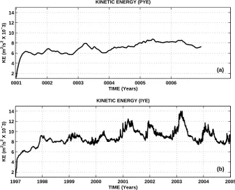
Both experiments have been studied, intercompared and compared with observations. One of the key indices of the circulation is the value of the kinetic energy over the Mediter-ranean basin. The Atlantic box circulation is neglected be-cause we consider the Atlantic box as a parameterization of large scale effects. Figure 5 shows the values of Kinetic En-ergy for (PYE), panel a) and (IYE), panel b). The values increase during the first months of simulation in both exper-iments. The Kinetic Energy reaches a more or less stable value in (PYE) after the third year of integration. The values for experiment (IYE) seem to reach a statistically flat trend after the first two years of its run. As expected, the values of Kinetic Energy are higher and have more variability in (IYE) than in (PYE), due to the fact that (IYE) is forced by the at-mospheric large scale interannual variability (PYE).
The first two years of (IYE) could be considered as the time necessary for the model spin-up; in the following
sec-tions we therefore show only the results from 1999. The sixth year of perpetual simulation will be considered as the refer-ence year for (PYE).
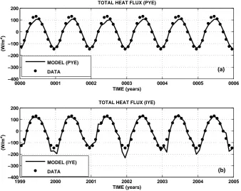
The model results were first compared with independent data sets for the heat and wind stress forcing. Figure 6 shows a time series of the total heat flux, described in Eq. (24) and computed as basin mean for (PYE) and (IYE) over a time period mean of one month. The model values are com-pared with the NCEP/NCAR re-analysis values (Kalnay et al., 1996). (PYE), panel a), does have lower values than NCEP/NCAR during the summer but it reproduces the sea-sonal cycle rather faithfully. (IYE), panel b), on the contrary, reproduces the summer well, and shows a large interannual variability in the winter fluxes, as was expected. Overall, we may say that the model is forced by consistent heat fluxes in both the (PYE) and (IYE) experiments.
The monthly wind stress mean over the basin is now ana-lyzed together with the monthly mean wind stress curl.
Jan Apr Jul Oct Jan 0.02
0.04 0.06 0.08 0.1
time (yr)
(N/m
2 )
WIND STRESS
(a) PYE NCEP
1999 2000 2001 2002 2003 2004 2005
0.02 0.04 0.06 0.08 0.1
time (yr)
(N/m
2 )
WIND STRESS
(b) IYE PYE
1999 2000 2001 2002 2003 2004 2005
0 0.5 1
time (yr)
(N/m
3*10e6)
WIND STRESS CURL
(c) IYE PYE
Fig. 7. Wind stress (N/m2) and wind stress curl (N/m3×106) from model simulations and NCEP-NCAR data as mean over the Mediterranean Basin. Panel (a): climatological monthly mean wind stress from NCEP-NCAR (thin line) and monthly mean from the sixth year of the perpetual forcing experiment (thick line). Panel (b): wind stress from model simulation from January 1999 to December 2004 (thick line) and the perpetual year simulation values (thin line). Panel (c): wind stress curl from the model simulations from January 1999 to December 2004 (thick line) and the perpetual year experiment (thin line).
1999 2000 2001 2002 2003 2004 2005 −0.1
−0.05 0 0.05 0.1
Sv
NET TRANSPORT AT THE STRAIT OF GIBRALTAR
(a)
1999 2000 2001 2002 2003 2004 2005
0.5 0.7 0.9
Sv
1999 2000 2001 2002 2003 2004 2005 0
0.06 0.12
N/m
2
(b)
TRANSPORT
WINDSTRES
1999 2000 2001 2002 2003 2004 2005
0.5 0.7 0.9
Sv
time (yr)
1999 2000 2001 2002 2003 2004 2005 −10
0 10
N/m
3 * 10
6
(c)
TRANSPORT
WIND CURL
Fig. 9. Baroclinic transport (Sv) at the Strait of Gibraltar and wind stress and wind stress curl as mean in the Alboran Sea. Panel (a): net
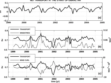
transport (eastward minus westward) at the Strait of Gibraltar over the period January 1999–December 2004. Panel (b): eastward transport at Gibraltar (thick line) and wind stress (thin line) as mean over the Alboran Sea (6◦W–1◦W) for the same period. Panel (c): eastward transport at Gibraltar (thick line) and wind stress curl (thin line) as mean over the Alboran Sea (6◦W–1◦W) for the same period.
note that the large amplitude meridional winds characteriz-ing the summer regimes over the Eastern Mediterranean are very weak in the NCEP/NCAR climatology, and this could explain the difference. The (PYE) forcing, calculated from ECMWF re-analysis (Korres et al., 2000), have the large am-plitude signal of the Etesian winds, however.
Panel b) represents the wind stress from (IYE) over the years 1999–2004 compared with (PYE). Both curves show a large seasonal signal but (IYE) shows a higher amplitude, especially during winter. The first three years of (IYE) are characterized by lower values of wind stress with respect to the final three years. Panel c) shows the wind stress curl from (PYE) and (IYE). The values of the wind stress curl are char-acterized by a seasonal signal and are mainly positive for the Mediterranean basin (as the basin is forced to have a cyclonic vorticity input). The years 2002, 2003 and 2004 have the largest wind stress curl values. In conclusion, we may ap-proximately say that the atmospheric forcing variability in (PYE) and (IYE) reproduces the well-known patterns and is consistent with an independent data set.
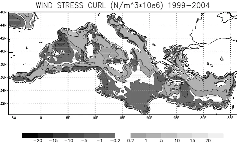
Figure 8 shows a map of the wind stress curl computed as mean over (IYE) from 1999 to 2004. The curl is posi-tive over a vast area of the northern part of the basin, with
the exception of the western part of the Gulf of Lion. The curl is mainly negative in the southern part of the Mediter-ranean, however. This is the well-known pattern of the wind stress curl over the Mediterranean (Pinardi and Mosetti, 2000; Demirov and Pinardi, 2002) that has been advocated in the past as the main cause for the cyclonic character of the basin-scale general circulation and anticyclonic circula-tion prevailing in the southern and south-eastern parts of the basin.
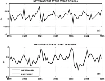
The mass transport at the main straits of the Mediterranean Sea is another important index of the basin scale circulation, and is also connected to deep and intermediate water forma-tion processes in the basin. The two main straits are the Strait of Gibraltar that connects the Mediterranean sea with the At-lantic Ocean and the Sicily Strait, subdividing the Mediter-ranean Sea into the western and eastern parts.
1999 2000 2001 2002 2003 2004 2005 −0.1
−0.05 0 0.05 0.1
Sv
NET TRANSPORT AT THE STRAIT OF SICILY
(a)
1999 2000 2001 2002 2003 2004 2005
0.5 1 1.5 2
Sv
WESTWARD AND EASTWARD TRANSPORT
(b) WESTWARD
EASTWARD
Fig. 10. Baroclinic transport at the Strait of Sicily (Sv). Panel (a): net transport for the period January 1999–December 2004 from the
interannual experiment. Panel (b): eastward (thin line) and westward (thick line) transport component at the Strait of Sicily from January 1999–December 2004.
the model the strait at its narrowest part is represented by 2 grid points). As explained in Sect. 2, special parameteriza-tions have been developed for this area. With a free-surface model, the net transport is different from zero and the inflow should be bigger than the outflow to balance the net water loss at the sea surface. The eastward and westward transport at the Strait of Gibraltar it is computed through a section at 6◦W. The net transport is the difference between these two components. It is shown in Fig. 9, and seasonal cycle is large and reaches maximum values in autumn. In March of some years, the net transport (panel a) may be negative, but the average values over the year are always positive. It is clear that the net transport has a large seasonal cycle with inter-annual fluctuations superimposed. The eastward and west-ward transport at the Strait of Gibraltar have approximately the same fluctuation with no clear evidence of a seasonal sig-nal. The variability of the eastward and westward transport is strictly related to the wind stress, as has already been pointed out in other works (Beranger et al., 2005). The wind stress and wind stress curl monthly mean have been computed over the area between 6◦W and 1◦W of longitude, correspond-ing to the Alboran Sea, for the years 1999–2004. Panels b) and c) of Fig. 9 show the value of the wind stress and the wind stress curl respectively superimposed with the eastward transport. It is evident that the variability of the transport is more strongly correlated with the wind stress curl than with the wind stress intensity. When the curl is strongly negative
(positive) the transport is high (low). When the curl is nega-tive (posinega-tive) the vorticity is anticyclonic (cyclonic) and the wind direction should be mainly eastward (westward). Jan-uary 2001 has a high transport and the curl is negative, whilst in December 2001 the transport reaches its minimum value and the curl is strongly positive, but in both cases (panel b) the wind stress is high. The time series of panel c) of Fig. 9 shows clearly how the correlation between the transport and the wind stress curl is well respected during all the period of study.
2000 2001 2002 2003 2004 2005 −40
0 40
steric (mm)
MODEL STERIC COMPONENT
(a)
IYE PYE
2000 2001 2002 2003 2004 2005
−20 20
SSH (mm)
MODEL SSH
(b)
IYE PYE
2000 2001 2002 2003 2004 2005
−100 0 100
time (yr)
SLA(mm)
SLA FROM MODEL AND SATELLITE
(c)
IYE SAT
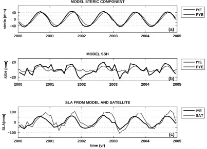
Fig. 11. Sea Level anaomaly mean over the Mediterranean basin for the period January 1999-December 2004. The unit of measure is mm.
Panel (a): steric componet variability computed for the perpetual year simulation (thin line) and the interannual year experiment (thick line). Panel (b): dynamic topography computed from the model sea surface high for the perpetual year experiment (thin line) and the interannual year (thick line). Panel (c): Sea level anomaly from January 1999 to December 2004 as mean over the Mediterranean basin from satellite monthly values (thin line) and model simulation for the same period (thick line).
of 1999–2001 from the observation and never less then 1 Sv from the model simulation for the same period.
Another way to assess the interannual model performance is to compare the model output with the satellite Sea Level Anomaly (SLA) time series. The model computes values of Sea Surface Height (SSH) without considering the steric ef-fect because it solves the incompressible continuity equation described in Eq. (4). Mass changes do not create a three-dimensional divergence and thus the steric effect is a diag-nostic quantity for our model. The steric component was then computed from the density field of the model and added to the SSH. Figure 11, panel a), shows the values of the steric component for both (PYE) and (IYE). The values are very similar for the two experiments and the seasonal cycle is clear with higher values during the summer. The values oscil-late between−40 mm in winter and +40 mm in summer. The area average values of SSH from the model are also shown in panel b), and in this case the difference between (PYE) and (IYE) is evident. The signal ranges between−25 mm and +20 mm in (IYE) and−5 mm and +10 mm for (PYE) show-ing that the sea level interannual signal is half of the steric seasonal signal in the Mediterranean Sea. In other words sea level variations induced by large scale circulation changes
produced by wind, water and heat fluxes over the Mediter-ranean Sea have half the amplitude of the steric seasonal ef-fects.
The SLA from the model has been defined as the sum of the steric component and the model SSH where every year its mean value has been subtracted. This time mean is equiv-alent to subtracting the mean sea level or mean dynamic to-pography of the model. This is done because the satellite altimetry values also have such value subtracted. Panel c) of Fig. 11 represents the comparison between (IYE) and the satellite data. (IYE) reproduces the seasonal variability and part of the interannual variability well but it is missing the high values during the late summer-autumn period.
Before discussing this mismatch, we would like to show the comparison of the model simulation with in-situ temper-ature and salinity profiles.
Jan030 Jun03 Jan04 Jun04 Dec04 1
2
° C
RMS TEMPERATURE XBT (data −model)
(a)
Jan030 Jun03 Jan04 Jun04 Dec04
1 2
° C
RMS TEMPERATURE ARGO (data −model)
(b)
Jan030 Jun03 Jan04 Jun04 Dec04
0.1 0.2
PSU
RMS SALINITY ARGO (data −model)
(c)
Jan030 Jun03 Jan04 Jun04 Dec04
0.5 1
kg/m
3
RMS DENSITY ARGO (data −model)
(d)
30m 150m 300m
Fig. 12. Rms error between data and model for year 2003 and 2004 at 30, 150 and 300 m depth. Panel (a): XBTs-model temperature rms
(◦C); panel (b): ARGOS-model temperature rms (◦C); panel (c) ARGOs-model salinity(psu); panel (d) ARGOs-model density rms (kg/m3).
in space of the data. The rms with the ARGO (Panel b), on the other hand, shows values lower than 0.5◦C, except in the summer, when the error is much larger at the depth of 30 m. This could be due to the misplacement of the seasonal ther-mocline in the model simulation. This situation is present also in panel c), which shows the rms for the salinity (Dobri-cic et al., 2007). The rms at 30 m is generally about 0.08 psu in September of both 2003 and 2004, and could reach a value of 1.6–1.8 psu. At 150 and 300 m the rms does not have this fluctuation. The rms at 150 m has values close to 0.08 psu with oscillation that could reach values of 1.2 psu or decrease down to 0.02 psu. At 300 m the rms is about 0.04 psu. Panel d) shows the rms of the density computed from temperature and salinity data from ARGO versus model. These values are well consistent with the results of salinity and tempera-ture discussed above.
We can now try to understand the differences in late summer-autumn in Fig. 11. This is due mainly to two fac-tors:
1. the wrong water flux during summer, which lacks the high evaporative fluxes during late summer and autumn;
2. the upper mixed layer physics, which does not correctly reproduce the relatively deep, hot and salty mixed layer during the summer-autumn period.
This interpretation is supported by the results of both Fig. 11 and Fig. 12, which show that the model has large model er-rors in the upper seasonal thermocline.
Figure 13 represents the velocity field at 30 m as averaged over 1999–2004. The model is able to reproduce the main circulation patterns of the Mediterranean Sea as described in the literature (Millot et al., 2005; Pinardi et al., 2004; Robin-son et al., 1002).
4 Conclusions
Fig. 13. Map of the circulation over the Mediterranean basin at 30 m computed as mean over the model simulation from 1999 to 2004.
model should be improved. This is the case of the water flux, which should be more realistic, and, as pointed out in Sect. 4, also of the model’s capability of the model to reproduce the hot and salty mixed layer during the summer-autumn period correctly. The computation of an SLA and the possibility to compare it to the satellite data is an important improve-ment with respect to the previous lower-resolution and rigid lid models implemented over the Mediterranean sea.
Appendix A
A1 Bathymetry and coastline
The Digital Bathymetric Data Base-Variable Resolution has been used to make the MFS1671 coastlines and bathymetry. DBDB-1 at 1’ resolution has been used for the Mediterranean basin, whilst for the Atlantic DBDB-2 and DBDB-5 have been used. The bathymetry file has been manually corrected along the Croatian coast by a comparison with detailed nau-tical charts. The bathymetry has been interpolated on the model horizontal and vertical grid and manually checked for isolated grid point, islands and straits and passages.
A2 Vertical level distribution
The distribution of the unevenly distributed vertical levels should satisfy the criteria of consistency and accuracy of the numerical scheme (Treguier et al., 1996). The vertical dis-tribution of the levels is computed in OPA by a function that has a nearly uniform vertical level distribution at the ocean top and bottom with a smooth hyperbolic tangent transition
in between. Several level distributions have been computed in order to find the one that reproduce the vertical shape of temperature and salinity profiles for the region best. Partic-ular attention has been paid to the intermediate layer resolu-tion where the water masses are characterized by only 0.5◦C anomalies in the western Mediterranean.
A3 Temperature and salinity monthly mean climatology
MEDATLAS monthly mean climatology
(MEDAR/MEDATLAS Group, 2002) and WOA98 (Lev-itus, 1998) gridded climatologies have been used for the Mediterranean Sea and the Atlantic Ocean respectively. The merging between the two climatologies has been done in a region on the western side of the Strait of Gibraltar.
A4 Wind stress and heat flux perpetual year climatology The wind stress monthly mean climatology has been per-formed with two different data set, one for the Atlantic and one for the Mediterranean. The monthly mean wind stress for the Mediterranean Sea has been computed by Korres and Lascaratos (2003) using the ECMWF re-analysis fields for the period 1979–1993. The monthly mean climatology from Hellerman and Rosenstein (1983) has been used for the At-lantic box. A weight function depending on distance in lon-gitude has been used to merge the two monthly data sets, and the data have then been interpolated with a spline on the nu-merical ocean model grid.
heat fluxes have been computed by Korres and Lascaratos (2003) using the COADS cloud cover data set for the period from 1980 to 1988 and the Reynolds SST.
Edited by: E. J. M. Delhez
References
Beranger, K., Mortier, L., Gasparini, G. P., Gervasio, L., Astraldi, M., and Crepon, M.: The dynamics of the Sicily Strait: a com-prehensive study from observations and model, Deep Sea Res. II, 51, 411–440, 2004.
Beranger, K., Mortier, L., and Crepon, M.: Seasonal variability of water transport through the Straits of Gibraltar, Sicily and Cor-sica, derived from a high-resolution model of the Mediterranean circulation, Prog. Ocean., 66, 341–364, 2005.
Castellari, S., Pinardi, N. and Leaman, K.: A model study of air-sea interactions in the Mediterranean Sea, J. Mar. Syst., 18, 89–114, 2000.
Demirov, E., Pinardi, N., Fratianni, C., Tonani, M., Giacomelli, L., and De Mey, P.: Assimilation scheme of the Mediterranean Fore-casting System: operational implementation, Ann. Geophys., 21, 189–194, 2003,
http://www.ann-geophys.net/21/189/2003/.
Demirov, E. and PInardi, N.: The simulation of the Mediterranean Sea circulation from 1979 to 1993. Part I: The interannual vari-ability, J. Mar Syst., 33–34, 23–50, 2002.
Dobricic, S., Pinardi, N., Adani, M., Tonani, M., Fratianni, C., Bonazzi, A., Fernandez, V.: Daily oceanographic analyses by the Mediterranean basin scale assimilation system, Ocean Sci., 3, 149–157, 2007,
http://www.ocean-sci.net/3/149/2007/.
Hellerman, S. and Rosestein, M.: Normal monthly wind stress over the world ocean with error estimates, J. Phys. Oceanogr., 13, 1093–1104, 1983.
Kalnay E., Kanamitsu, M., Kistler, R., Collins, W., Deeven, D., Gandin, L., Iredell, M., Saha, S., White, G., Wollen, J., Zhu, Y., Chelliah, M., Ebisuzaki, W., Higgins, W., Janoviak, J., Mo, K. C., Ropelewsy, C., Wang, J., Leetma Reynold, R., Jenne, R., and Joseph, D.: The NCEP/NCAR 40-Years Reanalysis Project, B. Am. Meteorol. Soc., 77, 437–471, 1996.
Korres, G., Pinardi, N., and Lascaratos, A.: The ocean response to low frequency interannual atmospheric variability in the Mediter-ranean Sea: Part I: Sensitivity experiments and energy analysis, J. Climate, 13, 705–731, 2000.
Korres, G. and Lascaratos, A.: A one-way nested, eddy resolving model of the Aegean and Levantine basins: Implementation and climatological runs, Ann. Geophys., 21, 1, 205–220, 2003.
Madec, G., Delecluse, P., Imbard, M., and Levy, C.: OPA8.1 Ocean general Circulation Model reference manual. Note du Pole de modelisazion, Institut Pierre-Simon Laplace (IPSL), France, 11, 1998.
MEDAR/MEDATLAS Group: MEDAR/MEDATLAS 1998-2001 Mediterranean and Black Sea database of temperature, salinity and bio-chemical parameters and climatological atlas (4CDroms), European Commission Marine Science and Tech-nology Programme, and internet server http://www.ifremer. fr/sismer/program/medarIFREMER/TMSI/IDM/SISMER Ed., Centre de Brest), 2002.
Millot, C. and Tapier-Letage, I.: Circulation in the Mediterranean Sea. Handbook of Environmental Chemistry, vol.5, Part K: 29-66, D=I 10.1007/b 107143, Springer-Verlag Berlin Heidelberg, 2005.
Pinardi, N., Allen, I., Demirov, E., De Mey, P., Korres, G., Las-caratos, A., Le Traon, P. Y., Maillard, C., Manzella, G., and Tzi-avos, C.: The Mediterranean ocean Forecasting System : first phase of implementation (1998–2001), Ann. Geophys., 21, 3– 20, 2003,
http://www.ann-geophys.net/21/3/2003/.
Pinardi, N. and Masetti, E.: Variability of the large scale general circulation of the Mediterranean Sea from observations and mod-elling: a review, Palaeo, 158, 153–174, 2000.
Pinardi, N., Korres, G., Lascaratos, A., Roussenov, V., and Stanev, E.: Numerical simulation of the interannual variability of the Mediterranean Sea upper ocean circulation, Geophys. Res. Lett., 24, 425–428, 1997.
Pinardi, N., Arneri, E., Crise, A., Ravaioli, M., and Zavatarelli, M.: The physical and ecological structure and variability of shelf ar-eas in the Mediterranean Sea, “The Sea”, Vol. 14, Chapter 32, 2006.
Reed, R. K.: On estimating insolation over ocean, J. Phys. Oceanogr., 17, 854–871, 1977.
Robinson, A., Malanotte-Rizzoli, P., Hecht, A., Nichelato, A., Roether, W., Theocharis, A., Unluata, U., Pinardi, N., and the POEM Group: General circulation of the eastern Mediterranean, Earth Sci. Rev., 285–309, 1992.
Roullet, G. and Madec, G.: Salt conservation, free surface, and varying levels: a new formulation for ocean general circulation models, J. Geophys. Res., 105(C10), 23 927–23 942, 2000. Sannino, G., Bargagli, A., and Artale, V.: Numerical modeling of
the semidiurnal tide exchange through the Starti of Gibraltar, J. Geophys. Res., 107, C5011, doi:10.1029/2001JC000929, 2002. Treguier, A. M., Dukowicz, J. K., and Bryan, K.: Properties of