www.atmos-meas-tech.net/8/1913/2015/ doi:10.5194/amt-8-1913-2015
© Author(s) 2015. CC Attribution 3.0 License.
On the microwave optical properties of randomly
oriented ice hydrometeors
P. Eriksson1, M. Jamali1,2, J. Mendrok2, and S. A. Buehler3
1Earth and Space Sciences, Chalmers University of Technology, 41296 Gothenburg, Sweden 2Division of Space Technology, Lulea University of Technology, 98128 Kiruna, Sweden
3Meteorological Institute, Center for Earth System Research and Sustainability, University of Hamburg,
Bundesstrasse 55, 20146 Hamburg, Germany
Correspondence to: P. Eriksson ([email protected])
Received: 2 December 2014 – Published in Atmos. Meas. Tech. Discuss.: 21 December 2014 Revised: 31 March 2015 – Accepted: 11 April 2015 – Published: 5 May 2015
Abstract. Microwave remote sensing is important for ob-serving the mass of ice hydrometeors. One of the main error sources of microwave ice mass retrievals is that approxima-tions around the shape of the particles are unavoidable. One common approach to represent particles of irregular shape is the soft particle approximation (SPA). We show that it is possible to define a SPA that mimics mean optical particles of available reference data over narrow frequency ranges, con-sidering a single observation technique at the time, but that SPA does not work in a broader context. Most critically, the required air fraction varies with frequency and application, as well as with particle size. In addition, the air fraction match-ing established density parameterisations results in far too soft particles, at least for frequencies above 90 GHz. That is, alternatives to SPA must be found.
One alternative was recently presented by Geer and Baordo (2014). They used a subset of the same reference data and simply selected as “shape model” the particle type giv-ing the best overall agreement with observations. We present a way to perform the same selection of a representative parti-cle shape but without involving assumptions on partiparti-cle size distribution and actual ice mass contents. Only an assump-tion on the occurrence frequency of different particle shapes is still required. Our analysis leads to the same selection of representative shape as found by Geer and Baordo (2014). In addition, we show that the selected particle shape has the desired properties at higher frequencies as well as for radar applications.
Finally, we demonstrate that in this context the assump-tion on particle shape is likely less critical when using mass
equivalent diameter to characterise particle size compared to using maximum dimension, but a better understanding of the variability of size distributions is required to fully charac-terise the advantage.
Further advancements on these subjects are presently dif-ficult to achieve due to a lack of reference data. One main problem is that most available databases of precalculated op-tical properties assume completely random particle orienta-tion, while for certain conditions a horizontal alignment is expected. In addition, the only database covering frequen-cies above 340 GHz has a poor representation of absorption as it is based on outdated refractive index data as well as only covering particles having a maximum dimension below 2 mm and a single temperature.
1 Introduction
The accuracy of the retrievals depends on technique ap-plied and a number of variables, including observational noise and limitations in the radiative transfer code used. However, for ice mass retrievals the main retrieval error sources are frequently uncertainties associated with the mi-crophysical state of the particles, i.e. phase, size, shape and orientation. This study focuses on the impact of assumed ice particle shape, probably the microphysical quantity with the least hope of being retrievable based on microwave data alone. Information on particle size can be obtained by com-bining data from different frequencies (Evans and Stephens, 1995a; Buehler et al., 2007; Jiménez et al., 2007), while the phase of the particles is largely determined by the atmo-spheric temperature. Measuring horizontal and vertical po-larisation simultaneously reveals whether the particles have a tendency to horizontal alignment or their orientation is com-pletely random (e.g. Hall et al., 1984; Hogan et al., 2003; Davis et al., 2005; Eriksson et al., 2011b).
Shape is normally not a critical aspect for purely liquid particles, as they are quasi-spherical throughout. The devia-tion from a strict spherical shape increases with droplet size and fall speed. However, the shape of frozen hydrometeors is highly variable, both as single crystals (needles, plates, columns, rosettes, dendrites, etc.) and as aggregates (see re-views by Heymsfield and McFarquhar, 2002; Baran et al., 2011). The shape is frequently denoted as the habit. It is un-likely that the air volume sampled contains a single ice parti-cle shape, i.e. a habit mix can be expected. Furthermore, this mix normally varies with particle size. In principle, the shape of each particle should be known to avoid a related retrieval error, but this is not a feasible goal. Instead some “shape model” must be applied and the main aim of this study is to examine such models for microwave sounding of pure ice hydrometeors.
Considering the ice particles to be solid spheres is prob-ably still the main microwave shape model. This approach is, for example, used in the standard 2B-CWC-O CloudSat retrievals by Austin et al. (2009). It is also applied in the Community Radiative Transfer Model (CRTM; Liu et al., 2013). Accordingly, retrieval systems (e.g. Boukabara et al., 2013; Gong and Wu, 2014) and radiance assimilation based on CRTM inherit the assumption of solid spheres. Further-more, this particle type has throughout been assumed in cloud ice retrievals based on limb sounding data (Wu et al., 2008; Rydberg et al., 2009; Millán et al., 2013). A main reason for the popularity of this shape model is that the single-scattering properties are simply calculated by well-established Mie codes.
Another common model is the “soft particle approxima-tion” (SPA) where the particles are treated to consist of a homogeneous mix of ice and air. This approach requires that the volume or mass fraction of air and the correspond-ing refractive index of the ice–air mix are determined; see Sects. 2 and 5. SPA could in principle be used with a range of simplified particle forms, but it seems that only spheres and
spheroids have been used so far. Spheroids are not treated by Mie theory but are covered by the also computationally ef-ficient T-matrix method (Mishchenko et al., 1996). One ap-plication of SPA for practical retrievals is Zhao and Weng (2002). A more recent example is Hogan et al. (2012), ar-guing for using a soft spheroid model for cloud radar in-versions. In addition, SPA has widely been used in studies to mimic measured radiances by radiative transfer tests (e.g. Bennartz and Petty, 2001; Skofronick-Jackson et al., 2002; Doherty et al., 2007; Meirold-Mautner et al., 2007; Kulie et al., 2010) in which the air fraction (AF) is either set to be fixed or derived from some parametric relationship between particle size and effective density.
Single-scattering properties for arbitrary particle shapes can be calculated e.g. by the discrete dipole approxima-tion (DDA; Draine and Flatau, 1994). DDA is used for incor-porating realistic particle shapes in the retrievals presented by Evans et al. (2012). This study is likely the most ambitious microwave retrieval set-up with regards to particle shape, but it deals only with a specific measurement campaign and it does not provide any general conclusions. Publicly available databases of DDA results for common particle shapes are re-viewed in Sect. 3. These databases have been used in dif-ferent ways: for example, Skofronick-Jackson et al. (2013) used one of the databases to estimate snowfall detection lim-its of several observation systems. Furthermore, the two main databases were used by Kulie et al. (2010) to test whether simulations could recreate some collocated radar and passive microwave data when applying different particle shapes. In a similar study by Geer and Baordo (2014), only passive data were considered but a more wide set of frequencies and at-mospheric conditions were investigated. They found that a sector-like snowflake model gave the smallest overall error for the simulations performed. This choice will replace a SPA treatment as the default for the snow hydrometeor category in the RTTOV-SCATT (Bauer et al., 2006) package (Geer and Baordo, 2014). In Sect. 6 an alternative version of the approach of Geer and Baordo (2014) is tested that does not involve any assumption on particle size distribution (PSD) or actual ice masses.
con-clusion has also been reached in indirect ways by others, as pointed out by Geer and Baordo (2014).
From the perspective of mass retrievals it is most practical to characterise the size of the particles through their equiva-lent mass ice sphere diameter,de:
de= 3
s
6m ρiπ
, (1)
wheremis the particle mass andρi is the density of (solid)
ice. We define the size parameter,x, correspondingly:
x=π de
λ , (2)
whereλis the wavelength at which the measurement is per-formed.
In microwave sounding, the mass is inferred from esti-mated extinction or backscattering coefficients. Any type of such coefficient,γ, can be expressed as
γ =
∞ Z
0
N (de)σγ(de)dde, (3)
whereN (de)is the PSD andσγ(de)is the local average cross
section for particles having a mass matchingde. In its turn,
Eq. (3) implies that trying to estimateσγ(de)from observed
satellite data (as done in Kulie et al., 2010; Geer and Baordo, 2014) requires a good knowledge of both the mass of frozen hydrometeors and the PSD.
Another common way to express particle size is by the maximum diameter,dm. We start the study by usingde, be-cause usage ofdmdemands that the relation betweendmand particle mass must be introduced. Such relationships depend on particle shape, and for the basic purpose of this study that is a problematic complication. By using de, particle shape
only influencesσγ(de). However, asdmis probably more
fre-quently used thande, this alternative to characterise particle
sizes is the last step of the study (Sect. 7).
In summary, our scope is the approximation of particle shape in microwave retrievals of the mass of pure ice hy-drometeors. Focus is put on SPA and the basic conclusion of Geer and Baordo (2014). Both passive and active mea-surements are considered, because merging information from different sensor types is already in use (e.g. Rydberg et al., 2009; Kulie et al., 2010), and such synergies should in the fu-ture just grow in importance. The practical aim can be seen as finding a shape model that gives a good estimate ofσγ(de),
for relevant optical properties, over a large range of parti-cle sizes, frequencies, measurement techniques and possible habit mixes. Existing DDA data are reviewed and used as reference. Only complete random orientation is treated be-cause most established publicly available DDA databases are currently limited to this assumption on orientation.
Furthermore, compared to earlier similar works, much higher attention is given to frequencies above 200 GHz.
Ice mass retrievals are already performed at sub-millimetre wavelengths using limb sounding (Wu et al., 2008; Rydberg et al., 2009; Millán et al., 2013) and airborne sensors (Evans et al., 2012). Additionally, a strong motivation for this as-sessment is upcoming sub-millimetre instruments: the Eu-ropean ISMAR (International Sub-Millimetre Airborne Ra-diometer) airborne instrument and the ICI (Ice Cloud Imager) sensor will be part of the next series of Metop satellites. ICI is a down-looking sub-millimetre cloud ice sensor, a concept that has already been described in several articles (Evans and Stephens, 1995a; Buehler et al., 2007, 2012) but for which so far no actual satellite sensor has been available. This study is part of our overall effort to build the scientific foundation for the analysis of first the ISMAR airborne and then eventually the ICI satellite data.
2 Refractive index
Any calculation of single-scattering properties, i.e. indepen-dently whether Mie, T-matrix or DDA calculations are per-formed, requires that the refractive index is specified. Param-eterisations and expressions related to the refractive index of ice at microwave frequencies are reviewed in this section. Both the real (n0) and imaginary (n00) part of the complex refractive indexnare relevant. Some relationships are more easily expressed in terms of the (relative, complex) dielec-tric constant,. Neglecting magnetic effects, which is a good assumption here, this quantity is related to the (complex) re-fractive index as
n=√. (4)
2.1 Pure ice models
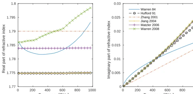
Providing complex refractive index practically over the com-plete electromagnetic spectrum in the form of data tables, Warren (1984), in the following referred to as W84, has been a long-term standard in atmospheric science for the refrac-tive index of pure water ice. Hufford (1991, H91) developed a parameterisation for microwave frequencies up to 1 THz based on Debye and Lorenz theories with parameters fitted from measured data. The parameterisation was incorporated in the MPM93 atmospheric propagation model by Liebe et al. (1993). Compared to W84, H91 generally predicts lowern00
for frequencies<350 GHz (see Fig. 1, right panel). Consis-tent with measurements it predicts a stronger increase ofn00
Frequency [GHz]
0 200 400 600 800 1000
Real part of refractive index
1.77 1.775 1.78 1.785 1.79 1.795 1.8
Frequency [GHz]
0 200 400 600 800 1000
Imaginary part of refractive index
0 0.005 0.01 0.015 0.02 0.025 0.03
Warren 84 Hufford 91 Zhang 2001 Jiang 2004 Matzler 2006 Warren 2008
Figure 1. Real (left) and imaginary (right) part of the refractive index of pure ice as a function of frequency, according to Warren (1984),
Hufford (1991), Zhang et al. (2001), Jiang and Wu (2004), Mätzler (2006) and Warren and Brandt (2008). The temperature is set to 266 K.
at sub-millimetre frequencies and atmospheric temperatures. Forn00they found a linear temperature dependence of about 1 % K−1. The measurements agree quite well with the H91 and J04 models. However, the Z01 model falls short of repro-ducing their own measurements – it predicts very low values over all frequencies (see Fig. 1) and all temperatures.
Mätzler (2006, M06) introduced a permittivity parameter-isation that consolidates most earlier models and measure-ments. Regarding the imaginary part, it agrees well with the J04 model, particularly at microwave frequencies, deviating by less than 5 % at higher frequencies and high temperatures. The largely revised and updated version of W84, the Warren and Brandt (2008, W08) data, incorporates the M06 model atT = −7◦C and proposes M06 as the model of choice at wavelengths beyond 200 µm when temperature dependence should be considered.
J04 found their model to be within 12 % of the imaginary permittivity measurements for frequencies below 800 GHz and within 15–40 % above 800 GHz. M06 estimated the un-certainty of their model from the standard deviations of mea-surements to 5 % at 270 K and 14 % at 200 K. W08 state the uncertainty of theirn00 data to be 10 % (T = −7◦C).
Com-pared to recent models, the once quasi-standard model W84 strongly overestimatesn00at millimetre wavelengths (up to a factor of 5), underestimates it at sub-millimetre wavelengths (up to a factor of 2) and overestimates it in the far-infrared (up to a factor of 2). The impact on particle absorption due to selection of M06 or W84 is exemplified below (Sect. 3.4). In contrast ton00,n0 is generally considered to be known with higher accuracy and to vary little to negligibly with both temperature and frequency. The measurements by Z01 confirm the small frequency dependence (0.3 % over 250– 1000 GHz) and do not show significant temperature de-pendence. The different models mentioned above provide slightly different relations ofn0with frequency and tempera-ture. However, we find refractivity (n0−1) from all models to
agree with M06 within 1.3 %, according to the left panel of Fig. 1. Based on estimates on propagation ofn0 uncertainty to optical properties, we conclude that the uncertainty inn0
is not a limiting factor and choice of model is not critical. In summary, M06 seems the best choice for microwave to far-infrared imaginary refractive index data. In view of the effects that errors in imaginary refractive index have on cloud optical properties (see Sect. 3.4), we strongly suggest no longer using the Warren (1984) data in future.
2.2 Mixing rules
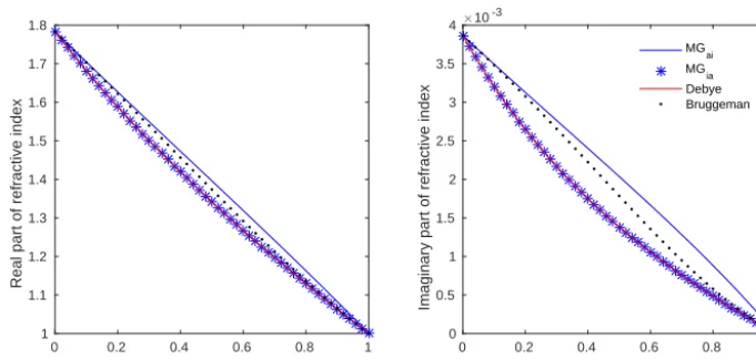
The parameterisations reviewed above deal with solid ice, while in the soft particle approximation (Sect. 5) the parti-cles are treated to consist of a homogeneous mixture of ice and air. The standard procedure for assigning a refractive in-dex to the mixture is to apply a so-called mixing rule. In this paper we compare some commonly used mixing rules from a purely practical perspective; a more theoretical review of mixing rules is provided by Sihvola (2000).
Throughout we will assume the refractive index of air to be 1+i0; in other words we assume that the optical properties of air are like those of a vacuum. Of course, for the radiative transfer problem as a whole both absorption and refraction by air matter strongly. However, given the much larger refractive index of ice we neglect this in the calculation of the single-scattering properties, as commonly done by other authors.
Three mixing rules are considered: “Maxwell-Garnett” (Garnett, 1906), “Bruggeman” (Bruggeman, 1935) and “De-bye” (Debye, 1929). All these formulas operate with dielec-tric constants. The Debye mixing rule is
e−1 e+2
=f
v 1(1−1)
1+2
+(1−f
v
1)(2−1)
2+2
, (5)
Air fraction [-]
0 0.2 0.4 0.6 0.8 1
Real part of refractive index
1 1.1 1.2 1.3 1.4 1.5 1.6 1.7 1.8
Air fraction [-]
0 0.2 0.4 0.6 0.8 1
Imaginary part of refractive index
#10-3
0 0.5 1 1.5 2 2.5 3 3.5 4
MGai MG
ia Debye Bruggeman
Figure 2. Real (left) and imaginary (right) part of the effective refractive index of a mixture of ice and air as a function of air volume fraction
according to some mixing rules. The refractive index of ice at 183 GHz and 263 K,nice=1.7831+i0.0039, was used, and the refractive
index of air was set tonair=1+i0.
and2arefor medium 1 and 2 respectively. The expression
for Bruggeman is
f1v(1−e) 1+2e
+(1−f
v
1)(2−e)
2+2e
=0. (6)
The Debye and Bruggeman expressions are symmetric with respect to the two media. Maxwell-Garnett differs in this respect by making a distinction between the “matrix” (=m) and the “inclusion” (=i):
e=m+3fivm (i−m)
i+2m−fiv(i−m)
, (7)
where isfivis the volume fraction of the inclusion medium (fmv+fiv=1). That is, for Maxwell-Garnett we have two cases, “air in ice” and “ice in air” (below shortened to MGai
and MGiarespectively), that result in differentedepending
on whether air is set to be the matrix or inclusion medium. For completeness, the effective density (ρe) matchingf1v
is
ρe=f1vρ1+(1−f1v)ρ2, (8)
whereρ1andρ2are the density of medium 1 and 2 respec-tively. In terms of mass fraction of medium 1 (f1m),ρeis
ρe=
ρ1ρ2
f1mρ2+(1−f1m)ρ1. (9)
An example comparison between the mixing rules is shown in Fig. 2. A first observation is that the Debye and the “ice in air” version of Maxwell-Garnett (MGia) give identical
results (form=air=1+i0 the two formulas are
mathemat-ically identical). Hence, the Debye rule is not explicitly dis-cussed below but is represented by the identical MGia. MGia
gives consistently the lowest refractive index for both real and imaginary part. The difference from the other two rules
is highest at air fractions around 0.45. The highest values are throughout found for MGai, and Bruggeman falls between
the two Maxwell-Garnett versions. Repeating the calcula-tions for other frequencies and temperatures (e.g. Johnson et al., 2012, Fig. 2), i.e. other ice refractive indices, shows that these patterns are of general validity and are not specific to our example.
The deviations between the mixing rules are significant. For example, Johnson et al. (2012) conducted a sensitivity analysis for frequencies between 2.8 and 150 GHz regarding the choice of mixing rule. The differences when using MGai
or MGia were found to be∼2 dB for radar reflectivity and
reach at least 10 K for brightness temperature.
Some mixing rule can be optimal for representing a true homogeneous ice–air spherical particle, as studied by Petty and Huang (2010), but this is not the crucial point in this context. In Sect. 5.1 we instead pragmatically test whether any of the mixing rules leads to a simpler approximation of realistically shaped particles.
3 Existing DDA databases
The DDA is the most widely used method for computing the scattering properties of arbitrarily shaped particles. In the DDA method, a particle is represented by an array of dipoles in a cubic lattice with a given inter-dipole spacing. This spacing must be adequately small relative to the inci-dent wavelength in order to obtain desired accuracy, which requires large computer memory and long calculation time for large particles.
Table 1. Overview of considered DDA databases.
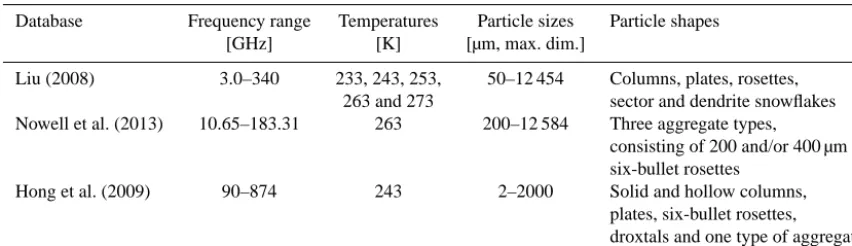
Database Frequency range Temperatures Particle sizes Particle shapes [GHz] [K] [µm, max. dim.]
Liu (2008) 3.0–340 233, 243, 253, 50–12 454 Columns, plates, rosettes, 263 and 273 sector and dendrite snowflakes Nowell et al. (2013) 10.65–183.31 263 200–12 584 Three aggregate types,
consisting of 200 and/or 400 µm six-bullet rosettes
Hong et al. (2009) 90–874 243 2–2000 Solid and hollow columns, plates, six-bullet rosettes, droxtals and one type of aggregate
The only other open source of microwave DDA data that we know about is http://helios.fmi.fi/~tyynelaj/, where data used in Tyynelä and Chandrasekar (2014) and some other publications were recently made available. These data, cov-ering frequencies up to 220 GHz, are not included in this pa-per as they deal with partly oriented particles, while the other databases all are valid for completely random orientation. 3.1 Liu
Liu (2008) applied the DDA code of Draine and Flatau (2000), denoted as DDSCAT, and computed single-scattering properties (i.e. scattering cross section, absorption cross sec-tion, backscattering cross secsec-tion, asymmetry parameter and phase function) of 11 types of ice particle crystal shapes, at 22 frequencies (3, 5, 9, 10, 13.4, 15, 19, 24.1, 35.6, 50, 60, 70, 80, 85.5, 90, 94, 118, 150, 166, 183, 220 and 340 GHz) and for five different temperatures. To not clutter the figures below, we include only 6 of the 11 particle types. The ig-nored shapes are: short column, block column, thin plate and four- and five-bullet rosettes; included shapes are pointed out in the figure legends. The included six particle types cover the full range of variation in the optical properties found in the database.
The particles were treated to have random orientation. The phase function is provided for 37 equally spaced scattering angles between 0 and 180◦. In terms of the “phase matrix” required for vector radiative transfer, only the (1,1) element is given. The refractive index of ice applied in the DDA cal-culation was taken from Mätzler (2006).
3.2 Nowell
A new snowflake aggregation model is introduced in Now-ell et al. (2013). The six-bullet rosette is a frequently ob-served crystal shape and therefore was selected by Now-ell et al. (2013) as constituent crystals of the simulated snowflake aggregates. The aggregates were allowed to grow in three dimensions, following an algorithm resulting in quasi-spherical snowflakes following the diameter-density parameterisation of Brandes et al. (2007). The representa-tion of the bullet rosettes is somewhat coarse, based on cubic
blocks with a size of≈50 µm. Only particles with a max-imum diameter above 1 mm are included in our figures to make sure that the aggregates consist of a relatively high number of building blocks.
The single-scattering properties of an ensemble of ran-domly generated aggregates were calculated by the DDSCAT code. Calculations for 10 frequencies (10.65, 13.6, 18.7, 23.8, 35.6, 36.5, 89, 94, 165.5 and 183.31 GHz) and a sgle temperature (263 K) were performed, with refractive in-dex taken from Mätzler (2006). The phase function is not included in this database; only the corresponding asymmetry parameter is stored.
3.3 Hong
Hong et al. (2009) also used DDSCAT to compute the scat-tering properties (extinction efficiency, absorption efficiency, single-scattering albedo, asymmetry parameter and scatter-ing phase matrix) of six randomly oriented non-spherical ice particles at 21 frequencies (90, 118, 157, 166, 183.3, 190, 203, 220, 243, 325, 340, 380, 425, 448, 463, 487, 500, 640, 664, 683 and 874 GHz) for a temperature of 243 K. All six in-dependent elements of the phase matrix are reported in steps of 1◦between 0 and 180◦.
The geometrical information of the six ice particle shapes is detailed in Table 1 of Hong (2007). Refractive index of ice was taken from Warren (1984), which according to Sect. 2.1 is not the optimal choice with respect to particle absorption.
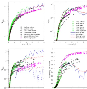
3.4 Comparison of the databases
x=:de=6
0 1 2 3 4 5 6
Q abs
10-3 10-2 10-1
Liu long column Liu thick plate Liu 3-bullet rosette Liu 6-bullet rosette Liu sector-like snowflake Liu dendrite snowflake Nowell aggregates
x=:de=6
0 1 2 3 4 5 6
Q sca
10-1 100 101
Hong column Hong hollow Hong plate Hong rosette Hong droxtal Hong aggregate Solid sphere Soft sphere Solid spheroid Soft spheroid
x=:de=6
0 1 2 3 4 5 6
Q bac
10-3 10-2 10-1 100 101
x=:de=6
0 1 2 3 4 5 6
Assymetry parameter
0 0.1 0.2 0.3 0.4 0.5 0.6 0.7 0.8 0.9 1
Figure 3. DDA-based single-scattering properties at 183 GHz from the databases of Liu (2008), Nowell et al. (2013) and Hong et al. (2009).
Absorption, scattering and backscattering efficiencies (Eq. 10) and asymmetry parameter are displayed. The combined legends are valid for all panels. The figure includes also data of solid and soft spheres and spheroids, with refractive index following Mätzler (2006). The soft particles have an air fraction of 0.75, with the effective refractive indices derived by the MGaimixing rule. The spheroids are oblate with an
aspect ratio of 1.67. All results are valid for 183 GHz and 243 K except those of Nowell et al. (2013) for 263 K.
as the corresponding efficiency,Q, calculated with respect to
deas
Q= 4σ
π de2
, (10)
whereσ is the cross section of concern. Even though usage of Qprovides some normalisation of the data, compared to when cross sections were to be plotted, the ordinates in the first three panels of Fig. 3 still span several orders of magni-tude. In Fig. 4 another normalisation is applied that brings out differences at lower size parameters: the optical cross sec-tions are divided by the corresponding optical cross section of the equivalent mass solid ice sphere with same ice refrac-tive index.
Although we discuss the soft particle approximation in depth only in Sect. 5, solid and soft spheroids are already included in the figures here for reference. We also already make some remarks on their optical properties here but
post-pone the explanation of how the soft-spheroid results were generated to the dedicated section later.
x=:de=6
0 0.2 0.4 0.6 0.8 1
r abs
0 0.5 1 1.5 2
Liu long column Liu thick plate Liu 3-bullet rosette Liu 6-bullet rosette Liu sector-like snowflake Liu dendrite snowflake Nowell aggregates
x=:de=6
0 0.2 0.4 0.6 0.8 1
r sca
0 0.5 1 1.5 2
Soft sphere, MG ai
Soft sphere, Brugg
Soft sphere, MG ia
Solid sphere
Hong column Hong hollow Hong plate Hong rosette Hong droxtal Hong aggregate
Figure 4. Absorption (left) and scattering (right) cross sections of DDA data and soft spheres at 183 GHz. The cross sections are reported
as the ratio to the corresponding cross section of the equivalent mass sphere, with the same refractive index as used for the preparation of the DDA data. That is, the dotted straight line atr=1 represents solid ice spheres. Database source and particle shapes of the DDA data are found in figure legends (same as in Fig. 3). The soft spheres have an air fraction of 0.25, where results for three different mixing rules (MGia,
Bruggeman and MGia) are included (solid lines).
It is well known that the impact of shape on the extinc-tion efficiency increases with particle size. Accordingly, for
xbelow∼0.5 there is a comparably low spread between dif-ferent particles for both absorption and scattering. In terms of the ratio in Fig. 4, the data are mainly inside 1.2±0.2.
However, at x=2 the difference between the lowest and highest scattering, for particles having the same mass, is about a factor of five (Fig. 3). These remarks consider also 340 GHz (not shown) where the same particles result in higher size parameters.
The backscattering efficiency shows a similar pattern as the scattering one, but the variation abovex=2 is consider-ably higher by about a factor of 10. This is the case because the backscattering depends on the phase function for a par-ticular direction, resulting in a higher sensitivity to the exact shape of that function, while the overall scattering extinction corresponds to the integrated phase function.
There is a significant spread in the asymmetry parameter (g) from aboutx=0.5 and above. Abovex≈1.5, the dif-ference between highest and lowest g is about 0.3, where the Nowell aggregates and the Liu bullet rosettes through-out cause the highest and lowest values respectively. The six-bullet rosettes in the Hong database show the same tendency of lowgfor combinations of size and frequency resulting in
x >1.5. At lowerxthe Hong rosettes tend to give the highest
gamong all of the particles, then also higher than the corre-sponding Liu rosette. That is, the different six-bullet rosette models used by Liu and Hong result in significantly different optical properties.
Figure 3 was inspired by Fig. 7 of Nowell et al. (2013), comparing that database with solid and soft particle calcula-tions in the same way. Nowell et al. (2013) used a higher air fraction for their soft particles and it is not clear whether the
MGai or MGia version of the Maxwell-Garnett mixing rule
was used, but there are still some clear deviations between the two figures for soft particles. For example, the scatter-ing efficiency of soft particles in our Fig. 3 is quite close to the data from Nowell et al. (2013), while in their Fig. 7 the soft particles give significantly lower scattering. In addition, we obtain basically identical scattering efficiencies for soft spheres and spheroids, while Nowell et al. (2013) got lower scattering for spheroids. We have carefully checked our cal-culations and our results seem to fit better with what has been found elsewhere. For example, in Fig. 5 of Liao et al. (2013) a good agreement with the aggregates of Nowell et al. (2013) is obtained by soft particles having a density of 0.2 g m−3 (the air fraction of 0.75 in Fig. 3 matches 0.23 g m−3), and basically identical results are obtained between spheres and both prolate and oblate spheroids.
4 Relevance of absorption and asymmetry parameter
Approximative size parameter [-]
0.00 1.01 1.37 1.70
Asymmetry parameter [-]
0 0.2 0.4 0.6
Cloud induced change [K]
0 20 40 60 80 100 120 140 160
Optical depth = 0.1 Optical depth = 0.5 Optical depth = 2.0
No absorption With absorption
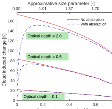
Figure 5. Test of importance of absorption and asymmetry
param-eter for passive microwave radiative transfer. The brightness tem-perature deviation from simulations with no cloud layer is reported, where a positive value in the figure corresponds to a decrease in ab-solute brightness temperature. The stated optical depths refer to the zenith extinction of the cloud layer. For solid lines, the imaginary part of the refractive index was set to 0, resulting in no cloud particle absorption. The simulations are described further in the text.
strong influence in radiative transfer of solar radiation (e.g. Kahnert et al., 2008). The quantity is also frequently reported in connection to passive microwave radiative transfer (e.g. Liu, 2004; Kim, 2006), but, to our best knowledge, the actual influence ofgfor such applications has not been investigated in a general manner. A simple test of this type is found in Fig. 5. The calculations were done with the DOIT (Discrete Ordinate ITerative method) scattering module of the ARTS radiative transfer model (Emde et al., 2004; Eriksson et al., 2011a). Satellite measurements at 150 GHz and an incidence angle of 45◦ were simulated. Temperature and gas profiles were taken from a standard tropical scenario (Fascod), and a 2 km thick “cloud” layer, centred at 10 km, was added. The selection of surface emission is not critical for these quali-tative calculations and for simplicity the surface was treated to act as a blackbody. A single particle size (monodisper-sive PSD) was used for each simulation, and the number of particles was adjusted to obtain the specified zenith optical depths. Spherical particles with an intermediate air fraction (0.4) were assumed, andde was varied to obtain a range of
g. Solid ice particles could not be used for this test as they don not give a monotonic increase ofgwith particle size, and neither providegabove 0.7 (Fig. 3).
The solid lines in Fig. 5 show how the brightness tempera-ture changes withgwhen the cloud optical depth is kept con-stant and all particle absorption is suppressed. The basic pat-tern is that the cloud impact on measured radiance decreases with increasingg. This makes sense as highgmeans that the up-welling emission from the lower troposphere is less
redi-rected compared to the case of more isotropic scattering at lowg; see Buehler et al. (2007) for a schematic figure and discussion of the radiative transfer for this measurement ge-ometry. It is hard to see in the figure, but there actually are some “wiggles” aroundg=0.65, showing that the relation-ship togis not completely monotonic. That is, several values ofgcan result in the same radiance.
In Fig. 5 the cloud impact forg=0 andg=0.6 differs by a factor of about 2. That is, changinggby 0.1 results in a∼10 % change in cloud impact. For low optical thickness the relationship between scattering cross section (σs) and ra-diance impact is close to linear. Accordingly, a 10 % error inσs and a 0.1 error in g are in rough terms equally im-portant. The test displayed in Fig. 5 was repeated for other frequencies and cloud altitudes. The absolute values of the cloud impact change, primarily following the magnitude of the gas absorption at the altitudes around the cloud layer, but the mentioned relation between σs andg was found to be relatively constant.
Figure 5 exemplifies also the importance of ice parti-cle absorption for passive measurements. It is well known that absorption is most significant for smaller particles, i.e. the single-scattering albedo increases with particle size (e.g. Evans and Stephens, 1995b; Eriksson et al., 2011b). Figure 5 confirms this as the difference between considering absorp-tion (dashed lines) and neglecting it (solid lines) is high for smallxfor all cloud optical depths. This aspect is especially important for limb sounding, because in this observation ge-ometry focus is put on higher altitudes where smaller parti-cles are more frequent, and it has been shown that the mea-sured signal can even be dominated by absorption (Wu et al., 2014).
Figure 5 also shows the less obvious fact that absorption increases in importance with increasing cloud optical thick-ness. For an optical thickness of 2.0 absorption is signifi-cant up to at least x=1.2, while for small optical depths (such as 0.1) the absorption can be neglected for x above ∼0.5. This is a consequence of the behaviour that probabil-ity of absorption increases when multiple scattering becomes more prominent. The changed conditions caused by multiple scattering implies that the relevance of absorption can not be judged alone from the single-scattering albedo parameter. In addition, the observation geometry matters for the rela-tive importance of absorption and scattering, as discussed in Eriksson et al. (2011b).
In summary, it is confirmed that the quantities normally considered (σa,σs,σb andg) are all relevant but to a
vary-ing degree. Most importantly, the relevance of absorption de-creases with size parameter.
5 Approximation by soft particles
0.6 0.7 0.7 0.8 0.8 0.9 0.9 1 1 1 1.1 1.1 1.2 1.2 1.3 1.3 1.4 1.5 1.6 1.7 1.8 MGai, absorption
x=:de=6
0.5 1 1.5 2
Air fraction [-]
0 0.1 0.2 0.3 0.4 0.5 0.6 0.7 0.8 0.9 0.2 0.3 0.4 0.5 0.5 0.6 0.6 0.7 0.7 0.8 0.8 0.9 0.9 0.9 1 1 1 1.1 1.1 1.2 1.2 1.3 1.4 1.5 MGai, scattering
x=:de=6
0.5 1 1.5 2
Air fraction [-]
0 0.1 0.2 0.3 0.4 0.5 0.6 0.7 0.8 0.9 0.3 0.4 0.4 0.5 0.5 0.6 0.6 0.7 0.7 0.8 0.8 0.9 0.9 0.9 1 1 MGia, absorption
x=:de=6
0.5 1 1.5 2
Air fraction [-]
0 0.1 0.2 0.3 0.4 0.5 0.6 0.7 0.8 0.9 0.1 0.2 0.3 0.4 0.4 0.5 0.5 0.6 0.6 0.7 0.7 0.8 0.8 0.9 0.9 0.9 1 1 MGia, scattering
x=:de=6
0.5 1 1.5 2
Air fraction [-]
0 0.1 0.2 0.3 0.4 0.5 0.6 0.7 0.8 0.9
Figure 6. Absorption (left) and scattering (right) cross sections of soft spheres (183 GHz and 243 K), normalised by the equivalent mass ice
sphere absorption or scattering cross section as in Fig. 4, as a function of size parameter and air fraction. The two top panels are calculated using the MGai(air in ice) mixing rule, while the two lower panels are calculated using the MGia(ice in air) mixing rule.
are considered, also water (e.g. Galligani et al., 2013). The air fraction of the mix is either set to a constant value or is obtained by assuming an effective density of the particle, likely varying with particle maximum size. A single refrac-tive index is assigned to the mix by applying a mixing rule (Sect. 2.2). Secondly, the particles must be set to have some specific shape, to allow the single-scattering properties to be determined with a limited calculation burden. As mentioned, the T-matrix method allows e.g. soft columns and plates to be possible options, but the standard choices are to model the particles as spheres or spheroids. A much more detailed description of SPA is provided by Liao et al. (2013). 5.1 Selection of mixing rule
As a first step, we examined whether the choice of mixing rule is critical in any way for SPA. The difference between mixing rules can in general be compensated by selecting dif-ferent air fractions, but exceptions exist. This is most clearly seen for the absorption and scattering cross section at smaller
x, as exemplified in Fig. 4. In the figure, the absorption of soft particles when using Maxwell-Garnet with “ice in air”
(MGia) is throughout lower than the DDA results. This is in
contrast to using the Bruggeman or the “air in ice” version of Maxwell-Garnett mixing rule (MGai), in which the soft
par-ticle absorption matches some of the DDA data points. The same pattern is found also for the scattering cross section but for a smaller range ofx.
The low bias in Fig. 4 of MGia, compared to DDA data,
can not be removed by modifying the air fraction, as shown in Fig. 6. In this figure, the ratios of Fig. 4 are calculated for air fractions between 0 and 0.95 and the ratios obtained when using MGiaare below 1 throughout. Ratios around at
least 1.2 are required to represent the average values of the DDA data in Fig. 4. Forx <0.5 such ratios, and even much higher values, can be obtained by selecting the MGaimixing
rule. Ratios when using Bruggeman (not shown) reach 1.25 for absorption and 1.15 for scattering, which is on the limit to fit the DDA data. For MGaithe ratios switch from being >1 to<1 aroundx=1, which in the following is shown to be the general behaviour of DDA data.
The conclusion of Figs. 4 and 6 is that using the MGia
same applies to the Debye mixing rule as it is identical to MGia. The Bruggeman rule gives higher values but is not
capable of reproducing the highest DDA-based ratios found in Fig. 4. The patterns seen in Fig. 6 are not specific to 183 GHz but are representative of the complete microwave region (1 to 1000 GHz). In addition, these remarks do not depend on whether soft spheres or spheroids are used. Ac-cordingly, MGai appears as the best choice in this context,
and only this mixing rule is considered below. 5.2 Selection of particle shape
Solid spheres are known to exhibit resonance features forx
above ∼1, which are reflected as oscillations in the prop-erties displayed in Fig. 3 (blue solid lines). An individual spheroid would give similar oscillations, but the assumption of completely random orientation partly averages out those patterns for the spheroids (see Fig. 3, red solid lines). The resonance phenomena are dampened when going to soft par-ticles. This results in a marginal difference in extinction (ab-sorption and scattering cross sections) and g between soft spheres and spheroids (dashed lines). However, there is a sig-nificant difference for the backscattering, where soft spheres give even stronger oscillations than solid spheres. The soft spheroids show a more smooth variation withx, and should allow a better fit to the DDA data. Liao et al. (2013) made the same observations for soft particles and showed that extinc-tion andgare basically unaffected by the aspect ratio of the spheroids or whether they are oblate or prolate. They found also that the oscillations in size dependence of the backscat-tering decrease when the aspect ratio moves away from 1.
That is, soft spheroids are preferable over soft spheres, pri-marily due to the difference with respect to backscattering. For complete random orientation the selection of aspect ratio is not critical, and only oblate spheroids with an axial ratio of 0.6 are considered below, following Hogan et al. (2012). In terms of the nomenclature used in the T-matrix code, this equals an aspect ratio of 1.67.
5.3 Selection of air fraction
As shown in the above figures, for a given size parameter there is a spread of the particle optical properties over the different habits. Hence, it is not possible to match all particle shapes at the same time with a soft particle approximation. The ambition is instead to approximately mimic the average properties. Figure 3 shows that solid spheres and spheroids do not meet this criterion because they (e.g. forx >4) sys-tematically underestimate scattering cross section andg.
It is stressed that in this work, air fraction is treated as a pure tuning parameter. This implies that statements about low/high air fractions just refer to values relatively close to 0/1; they are not judgements about the true density of the particles.
5.3.1 Relevance of the reference data
A more detailed analysis requires some consideration of the occurrence frequency of the different particles in the DDA databases. For example, the Hong database contains drox-tals having a maximum diameter, dm, up to 2 mm, while
the general view is that this shape is only representative for the smallest ice crystals (Baran, 2012). In fact, Schmitt and Heymsfield (2014) found that cloud ice particles with
dm above 250 µm are mainly the aggregate type, implying
that also single plates and columns having dimensions above this size are relatively rare. The aggregate types discussed by Schmitt and Heymsfield (2014) appear to be relatively simi-lar to the aggregates in the Hong database.
For the representation of particles of snow type, the Liu database offers two shapes (dendrite and sector-like snowflakes) that both have high aspect ratios, while the aggregates of the Nowell database (claimed to represent snowflakes) have an aspect ratio close to 1. This difference in aspect ratio results particularly in deviations in the scatter-ing cross section andgof those particles (Fig. 3). If “snow” is understood as everything from the classical single-crystal snowflake to graupel, both these assumptions on aspect ratio are realistic, but it is clear that particles having intermediate aspect ratios also exist and, hence, they are not yet covered by the DDA databases. The Hong aggregates could poten-tially also work as proxy for snow particles, but data fordm
above 2 mm are lacking.
5.3.2 Fit of single-scattering data
Figure 3 exemplifies a fit of the available DDA data using soft particles having an AF of 0.75. For the frequency of concern (183 GHz) the soft particles, compared to the solid ones, give indeed a better general fit of absorption and scattering effi-ciencies. Forgatx >1.5, the soft particles agree well with the Nowell aggregates, while all other particle shapes are bet-ter approximated with solid spheres or a comparably low AF. That is, for e.g. the Liu sector-like snowflake, the AF that gives the best fit with scattering efficiency is not the same AF that is needed to matchg.
Example results for other frequencies are found in Fig. 7. This figure, together with Fig. 4 covering 183 GHz, indicate that the MGaimixing rule combined with an AF of 0.25 give
x=:de=6
0 0.5 1 1.5 2 2.5
rabs
0 0.2 0.4 0.6 0.8 1 1.2 1.4 1.6 1.8 2
90 GHz
Soft spheroid, AF 0.25 Soft spheroid, AF 0.50 Soft spheroid, AF 0.75
x=:de=6
0 0.5 1 1.5 2 2.5
rsca
0 0.2 0.4 0.6 0.8 1 1.2 1.4 1.6 1.8
Soft spheroid, AF 0.90 Soft spheroid, H12 Solid sphere
x=:de=6
0 1 2 3 4 5 6
rabs
0 0.2 0.4 0.6 0.8 1 1.2 1.4 1.6 1.8 2
874 GHz
Soft spheroid, AF 0.25 Soft spheroid, AF 0.50 Soft spheroid, AF 0.75
x=:de=6
0 1 2 3 4 5 6
r sca
0 1 2 3 4 5 6
Soft spheroid, AF 0.90 Soft spheroid, H12 Solid sphere
Figure 7. Normalised absorption (left) and scattering (right). The top row includes 90 GHz Hong/Liu and 89 GHz Nowell data, while
the bottom row covers 874 GHz. The soft spheroids have either a fixed air fraction (AF) or follow Hogan et al. (2012), denoted as H12. Normalisation and plotting symbols used for DDA data are as in Fig. 4.
These remarks show three facts. Firstly, there is in gen-eral not a single AF that simultaneously gives a fit of all four optical property parameters. Secondly, at least when oper-ating at lower frequencies, the AF to apply in a soft parti-cle approximation must be allowed to vary with partiparti-cle size. Thirdly, the best AF has a frequency dependence (at least for largerx). The third point is well known and has been shown by e.g. Liu (2004).
The soft particle AF is frequently set to follow some den-sity parameterisation. This gives the AF a variation with size in line with the second point. However, the known fact that an optimal AF varies with frequency (point 3) signifies that using true densities cannot work as a general approach with respect to optical properties. This is the case because density-based AFs are independent of frequency. In addition, for larger particles standard density parameterisations result in much higher AFs than the ones giving a match of single-scattering data around 100 GHz and above. As an example, the particle model of Hogan et al. (2012) is included in Fig. 7. This particle model is based on the frequently used density
parameterisation of Brown and Francis (1995) that leads to AFs close to 1 for the largest DDA particles. In fact, the scattering efficiency at 90 GHz becomes too low already at
x≈0.5. Also, backscattering is underestimated atx above ≈0.5 even at lower frequencies (Fig. 8). All other density parameterisations we have tested show the same general fea-ture: to produce, in this context, too-high AFs for larger par-ticles. For more recent parameterisations the density goes be-low 100 kg m−3atdm≈800 µm (Cotton et al., 2013, Fig. 6).
Hogan et al. (2012) was selected as it provides a clearly de-fined particle model. However, it should be noted that Hogan et al. (2012) treat the spheroids to be aligned with the maxi-mum dimension in the horizontal plane, while we apply com-pletely random orientation.
5.3.3 Test radiative transfer simulations
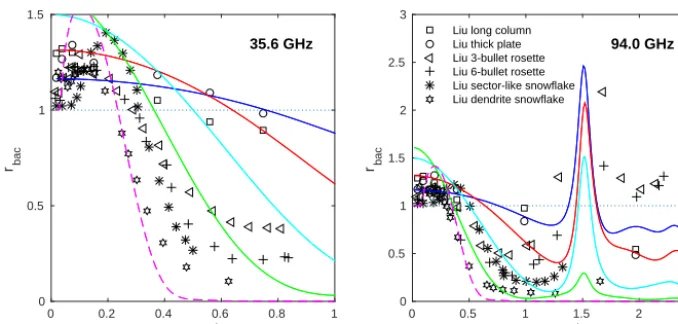
x=:de=6
0 0.2 0.4 0.6 0.8 1
rbac
0 0.5 1 1.5
35.6 GHz
x=:de=6
0 0.5 1 1.5 2 2.5
r bac
0 0.5 1 1.5 2 2.5 3
94.0 GHz Liu long column
Liu thick plate Liu 3-bullet rosette Liu 6-bullet rosette Liu sector-like snowflake Liu dendrite snowflake
Figure 8. Normalised backscattering of the Liu particles at two frequencies. As in Figs. 4 and 7, the normalisation is performed with respect
to the backscattering cross section of the solid sphere having the same mass. For 94 GHz andx≈1.5 some data points have a ratio above 3 partly due to a minimum of the solid sphere backscattering at that size parameter. Solid and dotted lines are the same as in Fig. 7.
in a positive or negative manner. These simulations, shown in Fig. 9, were performed for the same scenario as used for Fig. 5. Again, a monodispersive PSD was used, but here the number of particles was adjusted to obtain a specified verti-cal column of ice mass, or ice water path (IWP). The IWP for each frequency was selected to give a maximum cloud-induced brightness temperature change of 5–10 K in order to get a significant response but still avoid a high degree of multiple scattering.
As mentioned, the radiative transfer simulations were done with ARTS-DOIT (Sect. 4). This scattering method requires the full phase function and no results for the Nowell database could be generated. For Fig. 9 a more strict selection of the DDA particles was done, roughly matching the discussion in Sect. 5.3.1 in order to remove the less physically plausible particles. Column, plates and three-bullet rosettes havingdm
above 1 mm were excluded. For droxtals the limit was set to 200 µm. The black solid lines show a polynomial fit (in linear scale) of the simulations based on the remaining DDA particles.
As expected from the discussion above, the different DDA particles give little spread of simulated brightness temper-atures for x <0.5. However, there is a strong variation at larger size parameters. For example, the Liu dendrite snowflakes, as well the Hong six-bullet rosettes as around
x=1, have particularly low influences. This is a combined effect of relatively low scattering efficiency and high g
(Fig. 4). The same combination enhances also the differences between the Liu sector-like and dendrite snowflakes com-pared to the differences for scattering efficiency alone. The relative influence between the particles is not the same for all frequencies. For example, the Hong aggregates are found on the high side for 90 and 166 GHz but are rather on the low side for 874 GHz.
Figure 9 shows that the selection of the soft particle AF is not highly critical for size parameters below 0.5. This is partly due to compensating errors. A too-high AF gives an overestimation of both absorption and scattering, but this is counteracted by an overestimation of g. At higher size parameters, the frequency dependence of the “optimal” AF noted above is also seen here. For example, at 340 GHz an AF of 0.25–0.50 is required to match the fit of the DDA re-sults (black line), while for 90 GHz a suitable AF is above 0.75. For 874 GHz, only covered by the Hong database, an AF around 0.25 gives best agreement. The systematic devi-ation between the soft particle and the DDA-based results seen for 874 GHz and lowx is due to the refractive index differences discussed in Sect. 2.1.
6 Approximation by a single representative shape
Based on poor experience of using the SPA at ECMWF (the European Centre for Medium-Range Weather Forecasts), Geer and Baordo (2014) attacked the representation of parti-cle shape in microwave radiative transfer from another angle. Their application is data assimilation for numerical weather prediction, but the basic problem is the same as for direct re-trieval of frozen hydrometeors. Their approach is simple: to try to find a particle type, for which DDA calculations are at hand, that minimises the average deviation to actual ob-servations. They compared to measurements from the TMI and SSMIS sensors for frequencies between 10 and 190 GHz. The Hong database does not cover the lower end of this fre-quency range, and only the Liu database was considered.
x=:de=6
0 0.5 1 1.5
Cloud induced change [K]
10-1 100
101 90 GHz, 40 g/m2
Polynomial fit Soft spheroid, AF 0.25 Soft spheroid, AF 0.50 Soft spheroid, AF 0.75
x=:de=6
0 0.5 1 1.5 2 2.5 3
Cloud induced change [K]
10-1 100
101 166 GHz, 20 g/m2
x=:de=6
0 1 2 3 4 5 6
Cloud induced change [K]
10-1 100
101 340 GHz, 10 g/m2
x=:de=6
0 1 2 3 4 5 6
Cloud induced change [K]
10-1 100
101 874 GHz, 5 g/m2
Figure 9. Radiative transfer simulations at different frequencies. General conditions as in Fig. 5, i.e. a 2 km thick cloud layer at 10 km is
simulated. A single particle type is included in each simulation where the number density was adjusted to obtain the stated ice water paths. The black solid line is a high-order polynomial fit of the DDA-based results, while other lines are results for soft spheroids with constant air fraction (AF).
regions, land/ocean and the different hydrometeor types. Fur-thermore, a PSD must be assumed for the simulations. The tropical version of the PSD of Field et al. (2007) was found to give the best overall fit with observations among the three PSDs considered. These aspects introduce problems for a clear identification of the best overall proxy particle shape, as discussed in detail by Geer and Baordo (2014).
The final recommendation of Geer and Baordo (2014) is to apply the Liu sector-like snowflake for all classes of both cloud ice and snow. A somewhat better fit could be ob-tained by some combinations involving the six-bullet rosettes and dendrite snowflake particles, but the improvement was not sufficiently large to motivate a more complicated par-ticle shape model. Our results corroborate the selection of the sector-like snowflake as the general proxy shape particle. This particle type does not stand out in any obvious way; it shows in general intermediate values. In fact, the best match with the polynomial fit of the DDA-based simulations in Fig. 9 (black lines) is given by the sector-like snowflakes for both 90 and 166 GHz. A good fit is also obtained by the Liu
six-bullet rosette, another particle type that Geer and Baordo (2014) had as a strong candidate. The sector-like snowflake tends to be on the high end forxaround 0.7 but on the low side at higherx. If these happen to be true biases, they are partly averaged out in PSD-weighted bulk properties.
proxy shape because it has a very low scattering efficiency, aroundx≈1.5, which is also reflected in Fig. 9.
Figures 2 and 3 of Geer and Baordo (2014) complement the figures of this paper by reporting bulk optical properties of the Liu particles as a function of ice mass and frequency. A bit surprising is that the sector-like snowflake is found to have the lowest bulkg, seemingly for all frequencies and ice masses. This shape has also the lowestgamong the Liu par-ticles in Fig. 3 but only up tox=1.
Nevertheless, the SPA spheres applied are found to give very high bulkg. Geer and Baordo (2014) explain this as a re-sult of the Mie theory, but according to our Fig. 3 the highgis rather a result of the density assumed. The snow hydrometeor class is set to have a density of 100 kg m−3, corresponding to an AF≈0.9. We cannot easily judge the exact impact of this relatively high AF (meaning being close to 1, not that the true density is misjudged) for several reasons; e.g. Geer and Baordo (2014) used a mixing rule not considered by us. An-other complication is that the Field et al. (2007) PSD operates withdm. Hence, also differences in the relationship between
particle mass and dm between the particles affect the data
derived by Geer and Baordo (2014). There is a much more intuitive mapping of our findings to bulk properties whether the PSD is based onde.
Geer and Baordo (2014) analysed only passive observa-tions, while it would be highly beneficial if the representative shape selected could also be applied for radar measurements. Figure 8 indicates that this is the case. The backscattering of the sector-like snowflake follows its pattern for the scat-tering efficiency (Fig. 7). This shape has a ratio (as defined in discussed figures) above 1 up to a somewhat higher size parameter than the other particles and more pronounced at 35.6 than at 94 GHz; besides this, its properties are of aver-age character also with respect to backscattering.
7 Is using maximum dimension a better option?
Up to this point, we have compared radiative properties be-tween particles having equal de (thus also having the same
mass), for reasons discussed in the introduction. The second main measure for the size of individual particles is the max-imum dimension,dm. In fact, there are likely more PSDs us-ing dm than de. Hence, it is useful to also understand how the radiative properties vary withdm, and such an overview for 183 GHz is given in Fig. 10. This figure was produced as Fig. 3 but withdereplaced bydmin the definition of size parameter and absorption and scattering efficiencies.
The panels for asymmetry parameter in Figs. 3 and 10 are quite similar besides the range of x being extended when using dm. However, there are clear differences for both
ab-sorption and scattering efficiencies. There is a much more compact relationship betweendeand these radiative
proper-ties than what is found fordm. In the case of usingdmas the
size measure, relatively compact particles (droxtals, plates, columns and spheres) obtain especially high absorption and
scattering efficiencies, while particles having high aspect ra-tios (dendrite and sector-like snowflakes) exhibit especially low efficiencies. The stronger influence of particle morphol-ogy and aspect ratio results in a ratio between highest and lowest efficiency of ∼100 (besides for smallest particles). This is in clear contrast to Fig. 3, where the same ratios are around or below 10 when usingde(Sect. 3.4).
However, the higher variability in absorption and scatter-ing efficiencies is not directly mapped to the same variability in bulk optical properties, i.e. the optical properties of the dis-tribution as a whole. The reason for this is that particles with high aspect ratio have a lower mass as a function ofdm. This aspect deserves careful examination, so we analyse it in the remainder of this section. As a measure for the bulk optical properties we select the scattering extinction coefficient.
As an example of adm-based PSD we selected the trop-ical version of the PSD by Field et al. (2007), below de-noted as F07. The extinction coefficients were derived with a set-up basically identical to the one described by Geer and Baordo (2014) which also used the F07 PSD: only particles withdm≥100 µm were included (as the PSD does not cover
smaller particles), and the PSD was rescaled as described in their Appendix C to compensate for the truncation in particle size.
An additional aspect of the Field et al. (2007) size distri-bution is that it uses two additional input parameters,a and
b. They originate from the common way to express the rela-tionship betweendmand particle mass,m, as
m=admb. (11)
There are some issues around how to derivea andb for a particle type and how to perform the numerical integra-tions of the PSD. These issues are described carefully in Ap-pendix B and C of Geer and Baordo (2014) and there is no need to repeat all details. In short, we also selected to derive the a andb parameters by performing a functional fit, but only considering particles withdm≥100 µm. A reason to
ig-nore the smaller particles in the fit is that for them Eq. (11) may result indm< de(corresponding to density higher than
the one of solid ice) in cases where b <3. As Geer and Baordo (2014) did, we ensured that the bulk mass is pre-served by a rescaling of the PSD. This rescaling used the actual particle masses from the DDA database (i.e. assumed
aandbwere ignored in the rescaling).
However, not all dm-based PSDs take a and b into ac-count. To also investigate the impact of neglecting the depen-dence onaandb, bulk scattering was also derived with F07 and applying fixeda andb values for all particles, namely
a=0.069 andb=2. These values were selected following Wilson and Ballard (1999) and Field et al. (2007).
Since we want to compare dm-based and de-based bulk
extinction coefficients, we also need an example of a de
x0=:dm=6
0 5 10 15 20 25
Q'
abs
10-6 10-5 10-4 10-3 10-2 10-1
Liu long column Liu thick plate Liu 3-bullet rosette Liu 6-bullet rosette Liu sector-like snowflake Liu dendrite snowflake Nowell aggregates
x0=:dm=6
0 5 10 15 20 25
Q'
sca
10-4 10-3 10-2 10-1 100 101
Hong column Hong hollow Hong plate Hong rosette Hong droxtal Hong aggregate
x0=:dm=6
0 5 10 15 20 25
Q'
bac
10-4 10-3 10-2 10-1 100 101
Solid sphere Soft sphere Solid spheroid Soft spheroid
x0=:dm=6
0 5 10 15 20 25
Assymetry parameter
0 0.1 0.2 0.3 0.4 0.5 0.6 0.7 0.8 0.9 1
Figure 10. As in Fig. 3 but using the maximum dimension (dm) as characteristic size. That is, the size parameter is here defined asx0= π dm/λand absorption and scattering efficiencies are defined asQ0=(4σ )/(π dm2). As in Fig. 3, the frequency is 183 GHz.
to de-basis. Two combinations of a and b are considered: the first combination (0.0015/1.55) matches the sector-like snowflakes, having the lowest b among all the particles in the Liu database; the second combination (480/3) represents solid spheres and thus also the upper limit ofb. The rescaling to match specified ice water content has a marginal impact on F07. However, MH97 puts a much larger fraction of the mass below 100 µm and the rescaling gives a small but not negligi-ble change; therefore this PSD is displayed both before and after the rescaling. Like F07, MH97 is also a PSD targeting tropical conditions, and the agreement with F07 is relatively high fora=0.0015, b=1.55, while fora=480, b=3 the two PSDs deviate strongly.
Using the discussed PSDs, bulk scattering extinction coef-ficients can be calculated by adding up extinction coefcoef-ficients for individual particles with appropriate weights. Figure 12 shows the results: total extinction coefficients for the two dif-ferent PSDs, the dm-based F07 at the top and the de-based
MH97 at the bottom. For F07, results for fitted and fixed a
andbparameters are shown separately by straight and solid lines respectively.
As the top panel with the F07 results clearly demonstrates, the general pattern seen for the individual particles (Fig. 10) persists in bulk extinction: the more compact particles are at the upper end and the less compact (more “snowflake-like”) particles are at the lower end. However, as expected, the ra-tio between highest and lowest value decreased from∼100 when considering individual particles to∼10 when consid-ering bulk extinction. A similar spread in bulk extinction was obtained by Geer and Baordo (2014, see their Figs. 2 and 3). Still discussing the top panel of Fig. 12, we now turn to the issue of using fitted or fixeda andbparameters for the F07 PSD. For fixed parameters, the extinction obtained for particular shapes is changed, but the spread of the values is roughly maintained. It should here be noted that keepinga
andbfixed only has the consequence that the PSD gets the same basic shape for all particles. The rescaling to ensure that specified mass is matched maintains the relative fraction between particles having differentdm.
Equivalent sphere diameter [m]
10-4 10-3
Particle size distribution [1/m^4]
100 102 104 106 108
F07: a=1.5e-3, b=1.55 F07: a=480, b=3 MH97, rescaled MH97, original
Figure 11. Ice particle size distributions for 0.1 g m−3, according to Field et al. (2007, F07) and McFarquhar and Heymsfield (1997, MH97). The F07 PSD is converted fromdmtodefor two
combina-tions ofaandb(Eq. 11).
scattering for thede-based MH97 PSD compared to thedm
-based F07 PSD. The factor between highest and lowest ex-tinction in case of MH97 is∼2.5. This cannot be a conse-quence of MH97 putting the highest weight on completely different particle sizes, as the extinction using MH97 ends up inside the range resulting from F07. Furthermore, the rel-ative variability over the different habits is close to constant with ice water content, for both F07 and MH97, and already Fig. 11 showed that MH97 ends up inside the range cov-ered by F07 when a andb are varied. All in all, F07 and MH97 do a quite similar relative weighting between differ-ent particle size ranges. We therefore conclude that the dif-ference in spread seen between upper and lower panel of Fig. 12 is a direct consequence of the deviations revealed by Figs. 3 and 10; i.e. the scattering cross section is more closely linked todethan todm.
The difference betweendeanddm, exemplified by Fig. 12,
seems to be of general validity for frequencies up to ∼ 200 GHz. If anything, the difference increases when going down in frequency (not shown). At higher frequencies a somewhat different pattern is found for thedmcase, as shown in Fig. 13. Here at 340 GHz, the spread in extinction of the different DDA particles is overall lower compared to Fig. 12 and is particularly low at high ice water content, where it is even smaller than when using de. However, the dendrite snowflake particles constitute an exception, which is possi-bly an indication that this particular shape should perhaps be avoided for higher frequencies. In any case, the deviating re-sults for the dendrite snowflake show that the low spread in extinction between the other particles may be a coincidence, not necessarily indicating that usingdmensures low
uncer-tainty in extinction for high frequencies and high ice water content. Comparing usage of deanddmat high frequencies
Scattering extinction [1/m]
10-6 10-5 10-4 10-3
F07 PSD (d_m-based) 183 GHz
Fitted a and b Fixed a and b
Ice water content [g/m^3]
10-2 10-1 100
Scattering extinction [1/m]
10-6 10-5 10-4 10-3
MH97 PSD (d_e-based) Liu long column
Liu thick plate Liu 3-bullet rosette Liu 6-bullet rosette Liu sector-like snowflake Liu dendrite snowflake
Figure 12. Scattering extinction as a function of ice water
con-tent at 183 GHz for some of the particles of the Hong et al. (2009) DDA database. The particle size distribution applied in the upper and lower panels is F07 (Field et al., 2007) and MH97 (McFar-quhar and Heymsfield, 1997) respectively. Dashed lines in the up-per panel show results for the F07 distribution with fixeda=0.069 andb=2.
is presently complicated by the fact that the Hong database is limited todm≤2 mm and this size truncation can easily
cause artefacts in the comparison.
At the end of this section, we want to briefly mention two more general aspects of the problem of representing bulk par-ticle optical properties. Firstly, our analysis assumed that F07 and MH97 give an equally good representation of the mix of particle sizes. If in situ probes provide better data for either
de or dm, this should result in higher systematic errors for PSDs based on the more poorly measured particle size.
Secondly, besides possible systematic errors in the PSDs, the variability around average conditions must be considered. For example, it could be the case that there is a lower PSD variation (between locations, day-to-day, etc.) as a function ofdmthan as a function ofde. This situation would decrease,
or reverse, the advantage of usingde. If the opposite were
true, that PSDs tend to be more stable inde, this would
Ice water content [g/m^3]
10-2 10-1 100
Scattering extinction [1/m]
10-5 10-4 10-3 10-2
F07 PSD (d_m-based) 340 GHz
Fitted a and b Fixed a and b
Figure 13. As in Fig. 12 but for 340 GHz. The results for MH97 are
not shown as they show the same general pattern as in Fig. 12 (just shifted in mean level in the same way as the results for F07).
as we know, this important aspect of PSD variability has not been studied so far.
8 Summary and conclusions
We have reviewed the two most established databases of DDA calculations for microwave atmospheric radiative transfer, Liu (2008) and Hong et al. (2009). Nowell et al. (2013) is associated with the Liu database and was also con-sidered. All three databases assume completely random par-ticle orientation. The databases have different frequency cov-erage: Nowell from 10 to 183 GHz, Liu from 3 to 340 GHz and Hong from 90 to 874 GHz. Liu is the only database pro-viding data for more than one temperature. Scripts to convert the Hong and Liu data to the format expected by the ARTS forward model can be obtained by contacting the authors.
We noted clear systematic differences in absorption be-tween the Hong and Liu databases. The deviations are ex-plained by the fact that the refractive indices are based on different sources. Hong et al. (2009) used the data from War-ren (1984) that now are considered to be outdated. That is, we judge the only easily accessible DDA data above 340 GHz to be inaccurate on particle absorption. In the update of Warren and Brandt (2008), the parameterisation of Mätzler (2006) is recommended for the microwave region, and this is also the source of refractive index used by Liu (2008) and Now-ell et al. (2013). Another problematic aspect of the Hong database is the restriction todm≤2 mm.
We mainly compared optical properties between particles having the same mass and defined the size parameter (x) ac-cordingly (Eq. 2). For smallx below≈0.3, the variation of absorption and scattering between the particles is about 20 % (1.2±0.2 in terms of the ratio used in Figs. 4, 7 and 8). Go-ing towards higher x, the variation increases most quickly for backscattering, followed by scattering and finally most
slowly for absorption. At higherx, the ratio between low-est and highlow-est value is∼10,∼5 and∼2.5 for those three radiative properties respectively. The range in scattering is in general generated by the fact that particles of solid types have comparably high scattering, while shapes of “snow” char-acter result in low scattering. Kim (2006) found that solid spheres are representative up tox=2.5 (backscattering not considered and clearly allowing some systematic errors), but we, using a larger set of DDA calculations, find this limit somewhere aroundx=0.5.
We also scrutinised the soft particle approximation. A first conclusion was that the selection of mixing rule can lead to systematic errors at lowx. A mixing rule giving comparably high refractive index, for given air fraction, is needed to avoid this systematic error. We selected the Maxwell-Garnett with ice as the matrix and air as the inclusion media. With this selection of mixing rule, combined with an air fraction of about 0.25, SPA is applicable up to aboutx≈0.5 across the considered frequency range. This gives for absorption and scattering cross sections a maximum deviation to individual DDA calculations of≈30 %.
However, usage of SPA at higher x seems problematic. Each individual property calculated by DDA can likely be reproduced by adjusting the air fraction, but it is in general not possible to achieve a fit with several radiative proper-ties simultaneously. In any case, even fitting a single prop-erty, such as backscattering, requires that the air fraction is decreased when moving to higher frequencies. Thus, select-ing the air fraction based on some standard density param-eterisation can, in the best case, only work in a small fre-quency range. Our results indicate that this frefre-quency range then is found below 35 GHz as this approach leads to high AFs, passing 0.9 atdm∼1 mm. At very high frequencies, such as 874 GHz, an air fraction of 0.25 could potentially be applied for all particle sizes, but at lower frequencies the air fraction must also be adjusted with size, from about 0.25 at lowx(see paragraph above) to a higher value at higherx, for example 0.7–0.9 at 90 GHz. That is, applying SPA across the microwave region requires a model with a high number of tuning variables to give the air fraction the needed variation with frequency and size, while at the same time the resulting particle densities have no physical basis.