www.ocean-sci.net/3/491/2007/
© Author(s) 2007. This work is licensed under a Creative Commons License.
Ocean Science
Southern Ocean overturning across streamlines in an eddying
simulation of the Antarctic Circumpolar Current
A. M. Treguier1, M. H. England2, S. R. Rintoul3, G. Madec4, J. Le Sommer5, and J.-M. Molines5
1Laboratoire de Physique de Oceans, CNRS-IFREMER-UBO, Plouzan´e, France
2Climate Change Research Centre (CCRC), University of New South Wales, Sydney, Australia
3CSIRO Wealth from Oceans National Research Flagship and Antarctic Climate and Ecosystems CRC, Hobart, Australia 4Laboratoire d’Oc´eanographie et du Climat: Experimentations et Approches Num´eriques, Pierre and Marie Curie University, Paris, France
5Laboratoire des Ecoulements Geophysiques et Industriels, Joseph Fourier University, Grenoble, France Received: 9 July 2007 – Published in Ocean Sci. Discuss.: 17 July 2007
Revised: 5 December 2007 – Accepted: – Published: 19 December 2007
Abstract. An eddying global model is used to study the
char-acteristics of the Antarctic Circumpolar Current (ACC) in a streamline-following framework. Previous model-based es-timates of the meridional circulation were calculated using zonal averages: this method leads to a counter-intuitive pole-ward circulation of the less dense waters, and underestimates the eddy effects. We show that on the contrary, the upper ocean circulation across streamlines agrees with the theoret-ical view: an equatorward mean flow partially cancelled by a poleward eddy mass flux. Two model simulations, in which the buoyancy forcing above the ACC changes from positive to negative, suggest that the relationship between the resid-ual meridional circulation and the surface buoyancy flux is not as straightforward as assumed by the simplest theoret-ical models: the sign of the residual circulation cannot be inferred from the surface buoyancy forcing only. Among the other processes that likely play a part in setting the merid-ional circulation, our model results emphasize the complex three-dimensional structure of the ACC (probably not well accounted for in streamline-averaged, two-dimensional mod-els) and the distinct role of temperature and salinity in the definition of the density field. Heat and salt transports by the time-mean flow are important even across time-mean stream-lines. Heat and salt are balanced in the ACC, the model drift being small, but the nonlinearity of the equation of state can-not be ignored in the density balance.
Correspondence to: A. M. Treguier
1 Introduction
The meridional circulation of the Antarctic Circumpolar Cur-rent (ACC) is a key component of the global thermohaline circulation. It is believed to be comprised of two cells (Rin-toul et al., 2001). The upper one involves upwelling of deep waters south of the ACC, northward transport in the Ek-man layer and transformation into less dense waters (notably Antarctic intermediate water, AAIW). The second cell trans-forms upwelled deep waters into denser Antarctic Bottom Water (AABW) along the coast of Antarctica. The ampli-tude of the overturning cells is not well known for a num-ber of reasons. Firstly, air-sea fluxes are subject to large un-certainties, especially over the Southern Ocean. Secondly, data coverage is sparse: inverse models give some indica-tion of transport at 30◦S, but no circumpolar full-depth hy-drographic section is available south of that latitude, and es-timates at 30◦S vary considerably. Finally, mesoscale eddy fluxes are believed to play an important role in the meridional circulation, and measurements of those fluxes are available at only a few locations.
Table 1. Grid type and resolution of various models referenced in this paper. The name of the model is given with the resolution most
often quoted in the literature. The grid type refers to the southern hemisphere (OCCAM and ORCA025 have rotated or bipolar grids in the northern hemisphere). The Mercator grid is isotropic, i.e.,dyis refined asdxdecreases poleward.
Model Grid type dyat 60◦S Reference in this paper
POCM 1/4◦ lon,lat 44 km Jayne and Marotzke (2002) FRAM 1/3◦ lon,lat 28 km D¨o¨os and Webb (1994) OCCAM 1/4◦ lon,lat 28 km Lee and Coward, 2003 POP 1/6◦ Mercator 16 km Olbers and Ivchenko (2001) ORCA025 1/4◦ Mercator 14 km Barnier et al. (2006)
MESO 1/6◦ Mercator 9 km Hallberg and Gnanadesikan (2006) OCCAM 1/12◦ lon,lat 9 km Lee et al. (2007)
POP 1/10◦ Mercator 6 km Maltrud and McClean (2005)
using the FRAM model, showed that this cell is an artifact of zonal averaging, and involves branches of equatorward and poleward flow at the same depth but slightly different densi-ties that cancel out in the zonal average. It is thus necessary to consider the meridional circulation in density coordinates to study that part of the meridional overturning circulation that is relevant to water-mass transformation.
As an alternative, following the analogy with the Ferrell cells in the atmosphere, it is possible to calculate a resid-ual mean streamfunction (Mc Intosh and Mc Dougall, 1996). The definition most often used for the residual meridional velocity is
vRes=v− v
0σ0
σz
!
z
(1)
where v is the meridional velocity, σ the potential den-sity, the overbar represents an average (zonally and in time), prime represents the deviation about this average, and the subscriptzrepresents a vertical derivative. Mc Intosh and Mc Dougall (1996) show that to second order in the perturbation, this definition of the residual circulation is equal to the cir-culation averaged in density coordinates. However, the two definitions differ greatly in the surface mixed layer, because the vertical derivative ofσ appearing at the denominator in (1) vanishes. To complicate the picture further, both D¨o¨os and Webb (1994) and McIntosh and McDougall (1996) point out that in realistic models, the intensity of the circulation cells depends on the choice of density coordinates. D¨o¨os and Webb (1994) present circulations averaged at constant σ0 and σ3 (potential density referenced to the surface and 3000 m, respectively) and Mc Intosh and Mc Dougall (1996) use neutral density. As a result of those different methods, no consistent picture has emerged despite the publication of many meridional circulations from models (among others, D¨o¨os and Webb, 1994; Mc Intosh and Mc Dougall, 1996; Olbers and Ivchenko, 2001; Lee and Coward, 2003; Lee et al. 2007; Hallberg and Gnanadesikan, 2006).
The first aim of this study is to present a more coherent and complete picture of the meridional circulation in the ACC, by using a global model which brings together for the first time three important features: 1) an eddy-permitting model with an isotropic grid size of 14 km at 60◦S (see Table 1); 2) a coupled ocean-ice model with very well balanced, state-of-the-art atmospheric forcing; and 3) a long integration (44 years) allowing the ocean to adjust more thoroughly than in many previous studies with eddying models.
An eddying model is necessary because the residual mean meridional circulation has an eddy component. This appears clearly in (1), and the same is true in the isopycnal frame-work: in the latter case the transport is integrated over the instantaneous isopycnal thicknessesh, so that
vRes=v+ v0h0
h
=v+v∗ (2)
In recent years, a number of attempts have been made to build semi-analytic models of the meridional circulation of the ACC. Marshall (1997) proposed an idealized zonal av-eraged model, relating the strength of the meridional resid-ual streamfunction beneath the mixed layerhmto the surface density forcingD, such that
ψRes(−hm)= −
Z −hm
−H
vRes= D σy
(3) whereψResis the meridional residual streamfunction, H is the ocean depth andσy is the meridional potential density gradient in the mixed layer. (3) is derived from an equation for potential density, assuming a statistically steady state and no diabatic effects in the interior (see also Karsten and Mar-shall, 2002). Marshall (1997) illustrates (3) by two solutions, one with no surface density flux and zero meridional circu-lation (exact cancelcircu-lation of eddy and mean) and one with a cooling density flux that gives a net poleward meridional cir-culation in the upper layers. It is important to note that with the realistic geometry of the ACC the above model holds only when integrated following time-mean streamlines; in the zonal average one needs to take into account the corre-lationsvσ resulting from the permanent meridional excur-sions of the ACC (“standing eddies”). A further remark is thatDin (3) should include the lateral diabatic eddy fluxes in the mixed layer (Radko and Marshall, 2003). Karsten and Marshall (2002) use Southern Ocean observations to calcu-late the terms in (3). They estimate separately the mean and eddy component of the residual streamfunctionψRes. The mean streamfunction at the mixed layer base is taken to be equal to the Ekman transport:
ψ= − τ ρ0f
, (4)
whereτ is the wind stress,ρ0 the reference density and f the Coriolis frequency. The eddy streamfunction is parame-terized using the Gent and McWilliams formulation:
ψ∗= v
0σ0
σz
= −κσy σz
, (5)
whereκis a mixing coefficient, which Karsten and Marshall (2002) evaluate using observed sea surface height variability. The mean transport given by (4) is equatorward in the up-per layers in the whole Southern Ocean. Because the slope of isopycnals does not change sign, the eddy transport given by (5) is poleward. The residual circulation is thus the sum of two opposite contributions of the same order of magni-tude, and the sum is very dependent on the choice ofκin (5). Karsten and Marshall (2002) suggest that the eddies only par-tially compensate the mean in the southern part of the ACC, with a residual transport of 10 Sv equatorward, and that the eddies dominate the Ekman transport in the northern part, leading to a residual mean poleward flow of 10 Sv. Analyti-cal models based on (3)–(5) have been derived to explore the
influence of various forcings and boundary conditions (Mar-shall and Radko, 2003; Olbers and Visbeck, 2005). Olbers and Visbeck (2005) extend the model to take into account diabatic effects at the base of the surface mixed layer.
To our knowledge, the elegant conceptual model described in Eqs. (4)–(5) has never been tested in a realistic eddy resolving model. There have been only two attempts at calculating mean and eddy transports across streamlines. Ivchenko et al. (1996) used the FRAM model; they per-formed an analysis of the momentum balance across stream-lines but did not consider the surface circulation in detail. Lee and Coward (2003) obtain puzzling results with the OC-CAM 1/4◦model: they find that the time-mean meridional circulation dominates in the upper layers, and that the eddy contribution is important only at depth (1500 to 3000 m). Neither study has attempted to relate the meridional circu-lation to the model buoyancy fluxes. The eddy transports being dependent on model resolution, it is important to per-form new calculations of the meridional circulation across ACC streamlines using higher resolution models.
The aim of our study is to determine the upper ocean resid-ual circulation in the ACC belt using a streamline framework, and to document the extent of the cancellation between the eddy and mean flow. Our analysis concentrates on the re-gion of truly circumpolar flow, bounded by the northernmost and southernmost lines of constant barotropic tranport that go through the Drake Passage. Following Ivchenko et al. (1996) we call this area the “ACC belt”. We concentrate on the up-per meridional cell, also called the “Diabatic Deacon Cell” by Speer et al. (2000). We will try to relate this upper resid-ual circulation to the buoyancy forcing as in (3). We calculate the residual circulation in two solutions of the same model, but with different atmospheric forcings resulting in a differ-ent sign of the buoyancy flux over the ACC. We also calculate the balances of depth-integrated heat and salt and discuss the possibility of deriving a similar integrated balance for den-sity.
2 The numerical experiment
The global ORCA025 model is described in Barnier et al. (2006). This model configuration uses a global tripolar grid with 1442×1021 grid points and 46 vertical levels. Ver-tical grid spacing is finer near the surface (6 m) and increases with depth to 250 m at the bottom. The grid is completely isotropic in the Southern hemisphere; horizontal resolution is 27.75 km at the equator, 13.8 km at 60◦N, and gets to 7 km
−75 −70 −65 −60 −55 −50 −45 −40 −35 −30 −1
−0.5 0 0.5 1 1.5 2
Latitude
Density flux (10
−6
kg.m
−2
s
−1
)
Total Thermal Haline Total CORE
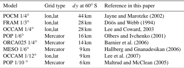
Fig. 1. Zonal average of the surface density flux (thick
continu-ous line), and the thermal and haline contributions (thin lines) for the reference experiment. The density flux of the CORE sensitivity experiment is indicated by the heavy dashed line. Positive values mean density gain for the ocean (buoyancy loss).
and a turbulence closure scheme (TKE) for vertical mixing. The bathymetry is derived from the 2-min resolution Etopo2 bathymetry file of NGDC (National Geophysical Data Cen-ter), merged with the BEDMAP data (Lythe and Vaughan, 2001) beyond 72◦S in the Antarctic.
The reference experiment considered in the present paper differs from the one of Barnier et al. (2006) because a dif-ferent forcing dataset is used. The experiment is interannual and runs from 1958 to 2002 with no spin-up (the initial con-dition is the Levitus 1998 climatology). The forcing dataset is a blend of data from various origins and different frequen-cies (Brodeau, 2007). Precipitation and radiation are from the CORE dataset assembled by W. Large (Large and Yea-ger, 2004), at monthly and daily frequency respectively. Pre-cipitation and radiation are based on satellite observations when available; a climatology of the same satellite dataset is used for the early years. Air temperature, humidity and wind speed are six-hourly fields from the ECMWF reanaly-sis ERA40. Turbulent fluxes (wind stress, latent and sensi-ble heat flux) are estimated using the CORE bulk formulae (Large and Yeager, 2004). To avoid an excessive model drift we add a relaxation to the Levitus climatology of sea surface salinity. The coefficient (0.167 m/day) amounts to a decay time of 60 days for 10 m of water depth; under the ice cover restoring is 5-times stronger. We also add extra restoring at the exit of the Red Sea and Mediterranean Sea because those overflows are not adequately represented at that model res-olution. A complete description of the experiment is found in a report (Molines et al., 2006). We have chosen to study a 10 year period from 1991 to 2000 (10 years is a sufficient period to compute eddy statistics; we prefer a period near the
end of the experiment so that the model drift is smaller). Un-less specified otherwise, “mean” quantities in this paper will refer to the 1991–2000 time-mean.
We also use a sensitivity experiment with the CORE “nor-mal year” climatological forcing (Large and Yeager, 2004). This forcing field is based on NCEP rather than ERA40 at-mospheric variables. The normal year is constructed by using the high frequency variability of 1992, with corrections so as to obtain annual mean fluxes close to the 1979–2000 clima-tology. There is no relaxation to climatological sea surface salinity under the sea ice in the CORE experiment, and the vertical mixing parameterization differs. The CORE sensi-tivity experiment is shorter (10 years); years 8 to 10 are used to calculate statistics.
It is always difficult to obtain a stable solution with a global ocean model forced by a prescribed atmosphere, be-cause the forcings usually have a nonzero average over the globe. Trying to balance the fluxes using observed sea sur-face temperature, as done by Large and Yeager (2004), is useful but does not prevent model drift. This is because the model fluxes during the integration are calculated with the model sea surface temperature which differs from the ob-served. The forcing fields for the long ORCA025 iment have been tested using low resolution model exper-iments (Brodeau, 2007) and the precipitation has been ad-justed in order to minimize the model drift. The experiment is run during 47 years without any “on-line” correction of the sea surface height (SSH). During the 10 year period con-sidered here, the global SSH increases by 11 cm due to a net sum of evaporation, precipitation and runoff of 0.12 Sv. This is a small flux imbalance compared, for example, with the total runoff (1.26 Sv). The global mean temperature de-creases by 0.011◦C due to a cooling of 0.09 PW (an average
of 0.25 W m−2) due to the direct surface heat flux, and a cool-ing of 0.06 PW (0.18 W m−2) due to the heat carried by the water exchanged through the free surface.
Regarding the ocean circulation, Barnier et al. (2006) show that ORCA025 represents the main ocean currents, the sea surface height and the surface eddy kinetic energy re-markably well. Indeed in some areas ORCA025 compares favorably with higher resolution models such as POP 1/10◦ (Maltrud and McClean, 2005). The good representation of the major fronts, together with the length of the reference ex-periment which ensures a weak drift, make it the most suit-able for our investigation of the residual circulation in the upper layers of the ACC.
In the southern part of the domain (south of 70◦S), the
model surface waters are made denser by cooling and by an input of salt. This input is partially due to brine rejection during ice formation, followed by ice export to the north; however a large contribution also comes from SSS relax-ation under ice, as shown by the difference between the ref-erence experiment and the CORE experiment (Fig. 1). In the latitude band 70◦S to 53◦S, the density flux is small (ref-erence case) or positive (CORE case). This agrees with a similar curve from a low resolution isopycnic model (Marsh et al., 2000, their Fig. 5), but many authors assume a net density loss in that latitude range (the density flux often used in idealized models, e.g, Marshall and Radko, 2003, is−2×10⁻⁷kg m2s−1). No reliable estimate of the density flux can be made from observations in that region, because it results of a near cancellation between cooling and freshen-ing, both of which are known only within large error bars. It is even unclear whether the heat flux between 55 and 65◦S
should be negative or positive. There is cooling in both our experiments (in the CORE case with NCEP air temperature as well as in the reference case with ERA40 temperature), while Speer et al. (2000) argue for a heating in that latitude band, based on the COADS dataset.
Farther north between 53◦S to 43◦S, the density flux is negative due to the combined effect of freshening and warm-ing. The warming is linked to a strong heat gain in the Malv-inas Current and south of the Agulhas retroflection region, in the Atlantic and Indian sectors. Although dismissed as a spu-rious feature by Gallego et al. (2004), such a warming shows up in a large number of datasets (Wacongne et al., 20071). It corresponds to an increase of the global ocean meridional heat transport (MHT) in that latitude band. This change in the slope of the global MHT curve is found in transports derived from atmospheric energy balances (Trenberth et al., 2001, their Fig. 13a and b) as well as in many high reso-lution global ocean model soreso-lutions (Maltrud and McClean, 2005; Lee et al., 2007; Meijers et al., 2007). Further to the north in the subtropical region, the density flux is again posi-tive because of a large heat loss and evaporation in the Brazil Current and in the Indian sector (in the Agulhas retroflection and its downstream extension). Generally, the surface fluxes in the Southern Ocean in the ORCA025 model, as well as the heat and freshwater transports, are within the admittedly large uncertainties of other published estimates.
3 Flow characteristics along the ACC belt
In this section we describe the ACC region in the reference experiment. The CORE sensitivity run is mentioned only when the results are significantly different. At the begin-ning of the reference run, the transport through Drake Pas-1Wacongne, S., Speer, K., Lumpkin, R., and Sadoulet, V.: Warm
water formation in the midst of the Southern Ocean, J. Mar. Res., submitted, 2007
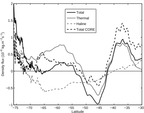
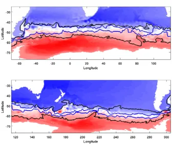
sage undergoes an adjustment: it decreases from 150 Sv to 115 Sv from 1958 to 1970. The transport remains stable af-terwards, with a 1991–2000 time average of 117 Sv. Fig-ure 2 shows two extreme contours of the barotropic stream-function going through Drake passage. We also indicate on this figure the Subantarctic Front, calculated as the south-ernmost extent of the salinity minimum, and the Polar Front, calculated as the northernmost extent of the temperature min-imum (calculated between 40 m and 400 m). The position of those fronts agrees overall with the estimates based on hy-drographic sections (Orsi et al., 1995) or sea surface height variability (Sokolov and Rintoul, 2007). The temperature minimum south of the polar front is simulated in the model, as shown by a section corresponding to the WOCE SR3 line between Tasmania and Antarctica (Fig. 3). Data from a jan-uary 1995 cruise (Sokolov and Rintoul, 2002) compare well with model results averaged during the same month. The temperature minimum in the model is found slightly higher in the water column than observed, especially at its north-ern end. The minimum temperature is warmer than observed (in the data, there is a significant thickness of water colder than 0◦C at 60◦S, which is not the case in the model). De-spite those discrepancies the model representation of the tem-perature minimum is very satisfactory compared with previ-ous experiments, such as the one described in Barnier et al (2006), where it was much too close to the surface. The im-provement has been brought about by a modification of the vertical mixing scheme to allow more penetration of the tur-bulent eddy kinetic energy (G. Madec, personal communica-tion). The lower panel in Fig. 3 shows the zonal velocity. The model has alternate bands of westward and eastward flow (about ten of them) in close agreement with the ten jets iden-tified by Sokolov and Rintoul (2007) from sea surface height. Indeed, a time-latitude plot of the meridional gradient of sea surface height (not shown) looks qualitatively similar to the observations (Sokolov and Rintoul, 2007; their Fig. 1). This confirms that the model resolution is sufficient to capture the scale of the main eddies and jets of the ACC.
Fig. 2. Time mean barotropic streamfunction (color). The black contours (7 Sv and 117 Sv) represent the limits of the ACC belt (circulation
that flows through Drake Passage). The Subantarctic Front (north) and the Polar Front (south) are indicated in blue (see text for definition).
in the Southern Ocean, it is important to sample the region south of the ACC belt, because most of the upwelling occurs there. Karsten and Marshall (2002) used geostrophic stream-lines and avoided closed contours by heavy smoothing and restricting their domain to 70◦S. Our high resolution model has its southern boundary at 80◦S and has well defined Ross and Weddell gyres, with many closed contours of barotropic streamfunction: using dynamics to define circumpolar con-tours south of the ACC belt is impossible. We have thus sim-ply defined 8 additional lines by interpolating linearly be-tween the ACC belt southern boundary (117 Sv contour) and the coast of Antarctica.
We have chosen barotropic streamfunction to define our streamlines because we prefer paths that are valid at all depths, in a vertically averaged view. At an early stage of this study we have also considered contours of sea surface height (as Karsten and Marshall, 2002) and the results were not sig-nificantly different. Using Bernouilli potential contours as Polton and Marshall (2007) would complicate the analysis since those contours would need to be defined differently on different isopycnals.
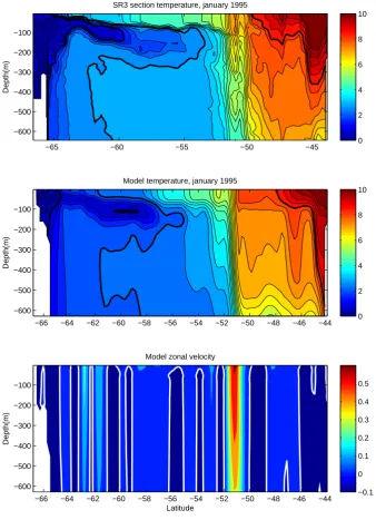
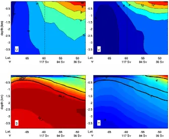
To investigate the meridional structure of the ACC, we present a few quantities averaged along those 20 lines. The sections are plotted as a function of the mean latitude of each line in Fig. 4. The top panels show the mean and rms
alongstream velocity. The velocities are quite small, even though the surface kinetic energy of the model is similar to satellite observations (Barnier et al., 2006) and the in-stantaneous velocities in the jets are large (note for exam-ple the maximum eastward velocity of 0.65 m/s along the SR3 section in Fig. 3). The streamline-averaged velocities are reduced because of meandering, and because the lines pass through regions of high and low velocities. There is no complex structure in these sections: velocities increase from south to north without showing multiple maxima. This is because we perform averaging along lines that are fixed in time. Meandering across those lines obscures the multiple jet structure, since the meridional scale of the meanders is not small compared to the spacing between jets (especially as the jets come close together at choke points, like in the Drake Passage). The bottom panels in Fig. 4 show salinity and tem-perature profiles, as well as three isopycnal surfaces (σ0=27, 27.5, and 27.7 kg m−3). The isopycnals cross the isotherms at a sharp angle resulting in large gradients of temperature and salinity along isopycnals. The salinity minimum corre-sponding to Antarctic Intermediate Water appears clearly in the salinity section.
Depth(m)
SR3 section temperature, january 1995
−65 −60 −55 −50 −45
−600 −500 −400 −300 −200 −100
0 2 4 6 8 10
Depth(m)
Model temperature, january 1995
−66 −64 −62 −60 −58 −56 −54 −52 −50 −48 −46 −44
−600 −500 −400 −300 −200 −100
0 2 4 6 8 10
Latitude
Depth(m)
Model zonal velocity
−66 −64 −62 −60 −58 −56 −54 −52 −50 −48 −46 −44
−600 −500 −400 −300 −200 −100
−0.1 0 0.1 0.2 0.3 0.4 0.5
Fig. 3. Observations and model results along the WOCE SR3 section. Top panel: observed potential temperature (January 1995).
Temper-atures of 0, 2 and 10◦C are indicated in bold. Middle panel: model potential temperature averaged for January 1995. Bottom panel: zonal velocities (m/s). The zero contour is underlined in white.
case and 25.4 Sv for the CORE case. The streamline average is not very different from the zonal average. Two thirds of the Ekman transport divergence (driving the upwelling) oc-curs south of the ACC belt. The density flux is shown in Fig. 5, top panel. For the reference experiment, the stream-line average results in a negative density forcing: the mean between 65◦S and 50◦S is−0.23×10⁻⁶kg m2s−1, close to the value used by Marshall and Radko (2003). Over the ACC belt (north of the limit indicated on the graph) there is a sharp
Fig. 4. Sections averaged following streamlines of the ACC, plotted as a function of the mean latitude of each streamline. In the two top
panels the vertical dashed line indicates the southern limit of the ACC belt. Top left: along-stream velocity. Top-right: rms velocity. Bottom left: contours of salinity (contour interval 0.1 PSU). Three isopycnals defined byσ0=27, 27.5 and 27.7 kg m−3are indicated by bold lines.
Bottom right: contours of temperature (contour interval 0.5◦C) with the same three isopycnals superimposed.
accurately the contribution of lateral diabatic eddy fluxes in the mixed layer from our model output, and thus consider only the contribution from surface buoyancy forcing in (3).
Before moving on to the meridional circulation, it is im-portant to note that the characteristics of the ACC vary strongly along its path. As discussed below, it is essential to take these along-stream variations of the ACC into account to understand the Southern Ocean overturning circulation and its relationship to surface forcing. Because eddy fluxes and upper ocean stratification are two important variables in de-termining the nature of the overturning circulation, we show the eddy kinetic energy (EKE) and mixed layer depth aver-aged over the ACC belt, both in the model and in observa-tions. The generally good agreement between the model and observations increases our confidence that the model cap-tures ocean physics sufficiently well to provide insights into the dynamics of the residual mean circulation.
The surface EKE varies along the path of the ACC by more than a factor of 10, in both model and observations (Fig. 6). The observed EKE is computed from satellite al-timetry (Ducet et al., 2000). Peaks of EKE are observed in the Agulhas (25◦E), near Crozet (60◦E), downstream of the Kerguelen plateau (75–90◦E), south of Tasmania and New Zealand (160 and 175◦E), downstream of Drake passage and
in the Brazil-Malvinas confluence zone (around 300◦E). The model successfully reproduces high EKE in all those regions, as already noted by Barnier et al. (2006). The CORE experi-ment has higher EKE than the reference. This may be partly due to stronger winds, but also to the shorter spin-up and/or internannual variability (consider the locally large difference between the two time periods indicated for the reference ex-periment).As noted by Hallberg and Gnanadesikan (2006), the large variations in EKE along the ACC path, with a spa-tial pattern clearly related to topography, suggest that insta-bility mechanisms active in the ACC are more complex than simple flat-bottom baroclinic instability. Eddies in the ACC likely depend on horizontal gradients of velocity (barotropic instability) and bottom topography as well as the vertical mean shear (classical baroclinic instability).
−70 −65 −60 −55 −50 −0.8
−0.6 −0.4 −0.2 0 0.2 0.4 0.6
Density flux (10
−6
kg.m
−2
s
−1
)
−70 −65 −60 −55 −50 −10
0 10 20 30
Ekman transport (Sv)
36 Sv 84 Sv
117 Sv Lat.
ψ
Fig. 5. Top panel: Streamline average of the surface density flux
(thick line), and the thermal (thin line) and haline (dashed line) contributions. The density flux of the CORE sensitivity experiment is indicated by the heavy dashed line. Bottom panel: streamline-averaged Ekman transport for the reference case (solid line) and the CORE experiment (dashed). The vertical dashed line indicates the southern limit of the ACC belt.
0 50 100 150 200 250 300 350 0
100 200 300 400 500 600 700
Longitude
surface EKE (cm
2/s 2)
Ref 91−2000 Ref 66−68 CORE TOPEX
Fig. 6. Surface eddy kinetic energy (EKE) averaged in the ACC belt
for each longitude. Data from altimetry, averaged over years 1992– 2002 is indicated by the thick black line. EKE for the reference experiment is shown for two time periods, 1966–1968 (years 8–10 of the experiment) and the reference period 1991–2000.
the model) in the southeast Pacific. The mixed layer in the CORE experiment is systematically shallower than in the ref-erence experiment, with the exception of a few regions of the south Pacific. As discussed below, the difference in the mixed layer depth appears to contribute to the differences in the residual circulation in the two experiments.
0 50 100 150 200 250 300 350 0
100 200 300 400 500 600
Longitude
September mixed layer depth (m)
Ref 91−2000 CORE Climatology
Fig. 7. Average mixed layer depth for the month of september, in the
model and in the climatology of de Boyer Mont´egut et al. (2007), estimated with a density criterion. The model mixed layer depth is estimated as the depth were density is 0.1 kg m−3larger than at the surface.
4 Meridional circulation in density coordinates
In this paper, we focus on the meridional circulation inte-grated in density classes. Formulation (1) is not used here because it breaks down in the surface mixed layer. An alter-nate formulation proposed by Held and Schneider (1999) and used by Marshall and Radko (2003) does not suffer from this problem. However, it involves the vertical velocity, which tend to be noisy near bottom topography in z-coordinate primitive equation models: this could make our results too dependent on the details of the numerical scheme. Rather, we choose the same method as Lee et al. (2007): the horizontal transport is binned in density classes for each 5-day model snapshot and averaged in time; the eddy contribution is then calculated by substracting the time-mean eulerian transport binned in the same density classes using the time-mean den-sity field. This method is robust and ensures that both mean and eddy components are consistent with mass conservation in the model.
−1000 −800 −600 −400 −200 0
Latitude
−70 −65 −60 −55 −50 −45 −40 −35 −30 −5000
−4500 −4000 −3500 −3000 −2500 −2000 −1500 −1000
Fig. 8. Zonal-mean meridional transport streamfunction calculated
in density space as a function ofσ2, and remapped as a function of
depth using the mean depth of theσ2surfaces. The top 1000 m is
expanded for visualisation. Positive values (black contours) indi-cate a clockwise circulation; negative contours are in grey. Contour interval is 2 Sv and the zero contour is indicated by a thick line.
transformation of Circumpolar Deep Water at the surface into Antarctic Bottom Water (AABW) which sinks to the bottom (see for example the cartoon by Speer et al., 2000). Note however that in fact, the existence and shape of the bottom cell in models is very dependent on a) how close to equilib-rium the model is; and b) how the model is forced. Regarding a), Lee et al. (2002) noted that the drift in deep water masses in an early version of OCCAM amounted to a deep cell of more than 20 Sv. The higher resolution model considered in Lee et al. (2007, Fig. 5) is analyzed after a very short spin-up period (three years). When we consider our model results after a spin-up period of 8 to 10 years (years 1966 to 1968 of the reference experiment, or years 8 to 10 of the CORE cli-matological experiment) we also obtain a cell that is continu-ous from the surface to the bottom, very similar to Lee et al., 2007. During the initial adjustment, the densest waters are flushed equatorwards and the slope of isopycnals decreases, leading to this enhanced bottom cell. Figure 8 shows the ref-erence solution averaged for the 1991–2000 period, after a spin up of 34 years, but the deep waters are still far from equilibrium. The structure and strength of the AABW cell also depend on the way deep waters are forced in the mod-els. In OCCAM 1/4◦ (Lee et al., 2003) the bottom cell is completely isolated from the surface and there is no surface cell of the same sign. The authors attribute this feature to the lack of an ice model and excessive diapycnal mixing. In the isopycnal model of Hallberg and Gnanadesikan (2006), there is a vigorous bottom cell extending all the way to the surface, but it is forced somewhat artificially by sponge layers near
the Antarctic shelf. The mechanisms of AABW formation and the related meridional circulation is a complex issue that will not be considered further here, as we now concentrate on the upper circulation cells.
A surprising feature in Fig. 8 is the counterclockwise cell in the upper 500 m between 45◦S and 63◦S. A similar cell appears in OCCAM 1/12◦(Lee et al., 2007) which the au-thors find “unusual” and do not attempt to interpret further. This circulation is also present in the isopycnic model of Hallberg and Gnanadesikan (2006). Those authors show that the cell is limited in its southward extent in low resolution models, but becomes stronger and extends farther south when the model resolution is increased (this is probably why it is absent in the lower resolution OCCAM 1/4◦ of Lee et al., 2002). In the OCCAM 1/12◦model, this cell is entirely due to the time-mean flow (permanent meanders), the transient eddy contribution being small excepted around 45◦S (Lee et
al. 2007, their Fig.5b). Hallberg and Gnanadesikan find that in their model both the time-mean and transient eddies con-tribute to this cell. Our model results thus confirm those two recent high resolution modelling studies; all three models show that in the range of latitudes of the ACC, the zonally-averaged transport in density coordinates is poleward near the surface, contrary to what is usually expected for the time-mean flow (an equatorward flow driven by the Ekman trans-port). Furthermore, the contribution of transient eddies is small compared to the mean. The explanation for this coun-terclockwise cell is the same as the one proposed by D¨o¨os and Webb (1994) for the Deacon cell, but this time applied to a calculation in density classes at constant latitude rather than a calculation at fixed depths. At a given latitude light water tends to go poleward, and is returned equatorward as denser water, so that the net result is a poleward transport of the more buoyant water. Summing the transport in density classes, we thus start with more poleward transport in the lighter classes. Because the ACC is highly non-zonal, there are large geostrophic velocities across a latitude line and the effect of those velocity-density correlations overcomes the Ekman transport (especially in high-resolution models where velocities are not excessively smoothed). As we will see, calculating the transport across mean streamlines rather than latitude circles more effectively reveals the physical nature of the meridional overturning in the upper ocean.
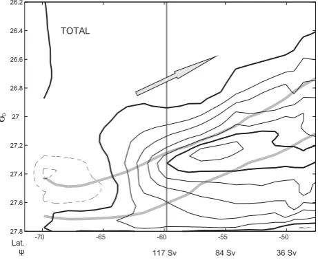
ψ
s
Fig. 9. Meridional transport streamfunction (time-mean flow only)
calculated in density space as a function of σ0, integrated along
streamlines and plotted as a function of the mean latitude of each streamline. Positive values indicate a clockwise circulation. Dashed contours indicate negative values. Contour interval is 2 Sv and the contours 0, 10 and 20 Sv are indicated by thick black lines. The thick grey lines indicate the 100 m and 500 m depth. The vertical line corresponds to the limit of the ACC belt.
(consider the vertical contours in Fig. 9 betweenσ0=27.6 and 27.8). As expected, integrating along streamlines reduces the amplitude of the time-mean velocity-density correlations. In the zonal mean view, one does not need to take eddies into account to eliminate the Deacon cell, it is enough to inte-grate the time-mean flow in density classes. In a streamline view, it is only when considering the total meridional circula-tion (mean + transient) that we can recover a consistent pic-ture without spurious deep upwelling or downwelling across time-mean isopycnals. Averaging zonally obscures the role of the transient eddies, while averaging following stream-lines more clearly reveals their influence.
The eddy-driven meridional circulation across streamlines is shown in Fig. 10. The eddy contribution is poleward as expected, in the opposite direction to the mean flow. In the resulting total streamfunction (Fig. 11) the spurious cross-isopycnal flow disappears. The residual circulation is 12 Sv equatorward, supplied by an upwelling along the sloping isopycnals at intermediate depths, south of the ACC belt. Our streamline-integrated view contrasts with the estimates of Lee et al. (2003) from the OCCAM 1/4◦ model. Their Fig. 5 shows a very small contribution of eddies in the up-per 500 m. This difference may be due to a lower resolu-tion of their model, or a less accurate determinaresolu-tion of their streamlines. Our reference experiment, when analyzed in a streamline framework, is in qualitative agreement with the “conventional” view of the meridional circulation across the
36 Sv 84 Sv
117 Sv Lat.
ψ
TRANSIENT
-70 -65 -60 -55 -50
-27.8 -27.6 -27.4 -27.2 -27 -26.8 -26.6 -26.4 -26.2
Fig. 10. Same as Fig. 9 for the transient meridional transport streamfunction calculated in density space as a function ofσ0,
in-tegrated along streamlines and plotted as a function of the mean latitude of each streamline.
ψ
s
Fig. 11. Same as Fig. 9 for the total (residual) meridional
trans-port streamfunction calculated in density space as a function ofσ0,
integrated along streamlines and plotted as a function of the mean latitude of each streamline.
−20 −10 0 10 20 −800
−700 −600 −500 −400 −300 −200 −100 0
Cumulated transport (Sv) 40 Sv streamline
MEAN EDDY
TOTAL
−20 −10 0 10 20 −800
−700 −600 −500 −400 −300 −200 −100 0
Cumulated transport (Sv) 100 Sv streamline
MEAN EDDY
TOTAL
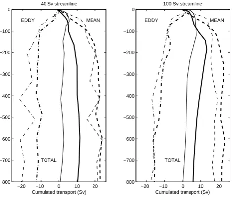
Fig. 12. Meridional transport streamfunction profiles, calculated in
density space as in the previous figures, but replotted as a function of the isopycnal streamline-averaged depths. Two experiments are compared (the reference, bold lines; and the CORE experiment, thin lines). For both experiments the mean, eddy and total (residual) overturning are indicated by dashed, dashed-dotted, and continu-ous lines respectively. Left-hand panel: circulation across the 40 Sv ACC streamline, with average latitude 50.1◦S.; right-hand panel, circulation across the 100 Sv ACC streamline, with average latitude 57.2◦S.
Although the general picture fits with idealized models such as Marshall (1997) or Karsten and Marshall (2002), there is no quantitative agreement between our model solu-tion and the simplified Eq. (3). In the equilibrium solusolu-tion (3), the residual circulation changes sign when the buoyancy forcing changes sign. This is not the case when we compare our reference experiment with the CORE one. The resid-ual circulation is weaker in the CORE run but still poleward, reaching 6.4 Sv on average in the core of the ACC. One ques-tion we want to point out about (3) is, at which depth should it be applied? It is apparent from Figs. 9–11 that both the mean and eddy overturnings have a complex vertical structure, so that the maximum residual circulation is set not only by the maximum mean and eddy component, but also by the way they compensate each other at different depths (or densities). Figure 12 compares profiles of cumulative transport (in-tegrated from the surface) across two ACC streamlines for the reference and CORE experiments. In both experiments the equatorward transport by the mean flow is partially com-pensated by poleward eddy transport. The mean equator-ward transport is larger in the reference case, in accordance with the slightly larger Ekman transport (Fig. 5). Hallberg and Gnanadesikan (2006) find that an increase in the Ekman transport leads to an increase in the opposing eddy flux; this is not the case in our experiments. The most striking
differ-ence between our two experiments is the vertical structure of the circulation. The residual transport increases much more rapidly from the surface in the CORE run, creating a maxi-mum near 60 m as opposed to about 200 m in the reference run. The residual streamfunctions for the two experiments diverge most dramatically between 100 and 200 m. In the reference case, the eddy transport is small in this depth range while the mean transport continues to increase with depth; as a result the residual circulation increases to a maximum near 200 m. In the CORE experiment, the eddy transport increases with depth more rapidly than the mean transport below 100 m, and the residual streamfunction is reduced to small positive values by 200 m depth. The larger eddy trans-port in the CORE case is consistent with the enhanced eddy energy in this run (Fig. 6).
The fact that the overturning streamfunctions differ most in the upper 200 m in the two experiments suggests the struc-ture of the mixed layer may contribute to the different circu-lations. While the maximum mixed layer depths are simi-lar in the reference and CORE cases, the annually averaged mixed layer depths are much shallower in CORE. This is likely due to the change in vertical mixing scheme (rather than the change in forcing), which was implemented with the specific objective of improving the summer mixed layer depths that were shallower than observed in the CORE run. Unfortunately, the ORCA025 model is too costly to perform multiple sensitivity experiments, changing one parameter at a time. In any case, the difference between the two runs il-lustrates that the relationship between the meridional circula-tion and buoyancy fluxes is not independent of the structure of the mixed layer and therefore vertical mixing, a fact il-lustrated by Olbers and Visbeck (2005). This dependency is hidden in equation by assuming that the relationship is valid at the base of the mixed layer. But in the real world, the mixed layer depth varies significantly with season and along streamlines (Fig. 7), so it is not possible to a priori decide at which depth the theory should be applied. In their ana-lytical model, Olbers and Visbeck (2005) have tried to take into account mixing at the mixed layer base by considering a transition layer in which the isopycnal slopes change from infinity (in the mixed layer) to their interior values. They find that the simplified Eq. (3) does not hold in the presence of such a transition layer, even without breaking the zonal symmetry of the problem. Furthermore, we have used only the surface buoyancy forcing in (3) but Radko and Marshall (2003) estimate that diabatic eddy fluxes in the mixed layer are likely to represent a significant contribution.
5 Depth-integrated balances
in a numerical model it is necessary to store all the tendencies of the temperature and salinity equation terms at every grid point, which is not yet feasible in a global eddy-resolving model (such diagnostics are used by Iudicone et al., 2007 in a low resolution version of the same model). The largest diffi-culty comes from the vertical mixing terms, which are highly nonlinear due to the turbulent closure scheme and cannot be estimated from our archived 5-days output. It is still possible to consider depth integrated balances (in which case the ver-tical mixing term vanish idenver-tically). This is of interest for two reasons. First, heat and salt transports have only been published so far integrated in latitude bands, not following the ACC path. Second, the theoretical model expressed in Eqs. (4)–(5) relies on an equation for conservation of poten-tial density written in flux form, which does not exist: inte-gral conservation statements can be written for potential tem-perature and salt, but a similar equation for density contains additional source and sinks due to thermobaric and cabelling effects. In this section we try to evaluate the importance of the nonlinearity of the equation of state for the evolution of density in the whole ACC belt.
Table 2 shows various depth-integrated balances across the ACC belt for both the reference and the CORE experiment. Regarding the net water balance, the ACC belt gains water at a rate of 0.4 Sv, which is compensated by an equivalent ex-port northward. The small residual is the drift due to the rise of global sea surface height during that period. In the ref-erence experiment the ACC belt loses heat through the sur-face flux at a rate of 0.11 PW. This is not compensated by the divergence of lateral heat transport (0.01 PW), nor by the heat content drift (0.01 PW). Rather, the surface cooling is compensated by the diffusive flux of heat along isopycnals. The model being eddy permitting, we have kept a Laplacian parameterization of isopycnal diffusion of potential temper-ature and salinity. This term being nonlinear, it is not pos-sible to calculate it exactly from the 5-day average ouput of the model. The mixing coefficient at the northern latitude (−47.6◦S) is 200 m2s−1. A rough calculation shows that with our Laplacian mixing coefficient a flux of 0.1 PW is ob-tained with an isopycnal gradient of temperature of 1◦C over a distance of 1000 km, which is compatible with the strong gradients shown in Fig. 4 at the northern boundary of the ACC. This value is also compatible with the eddy diffusive heat transport calculated by Lee et al. (2007) from the OC-CAM 1/12◦model. The importance of parameterized isopy-cnal diffusion is similar in the CORE case.
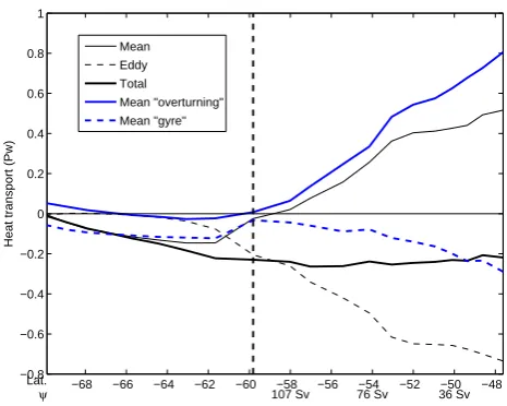
The eddy contribution to advective heat transport is also indicated in Table 2; it is the dominant contribution. At the northern boundary there is a large cancellation between the eddy flux (bringing heat southward) and the mean flux (bringing heat northward). This agrees with the conventional picture of the ACC, and with zonal mean curves of heat trans-port from various models that show a maximum eddy contri-bution just south of 40◦S (Jayne and Marotzke, 2002; Lee et al, 2007). The poleward eddy heat transport (0.73 Pw north
−68 −66 −64 −62 −60 −58 −56 −54 −52 −50 −48 −0.8
−0.6 −0.4 −0.2 0 0.2 0.4 0.6 0.8 1
Heat transport (Pw)
36 Sv 76 Sv
107 Sv Lat.
ψ
Mean Eddy Total
Mean "overturning" Mean "gyre"
Fig. 13. Meridional depth-integrated heat transport across
stream-lines for the reference experiment. The total and eddy part corre-spond to the numbers in Table 2 for the north and south boundary of the ACC region (this south boundary is marked by a vertical black line). The time-mean heat transport (thin black line) is further de-composed into two terms, the “overturning” and “gyre” parts.
Table 2. Balances in the ACC belt for the reference and the CORE experiments. For advective fluxes, the first number is the total and the
eddy contribution is indicated between braces. The flux convergence is the flux at the northern boundary minus the flux at the southern boundary; the sum of convergence and drift is expected to match the surface flux for the water, heat and density balance. For the salt balance the surface flux acts on local salinity but not on the integrated quantity of salt (it is indicated for completeness but marked with an asterisk). The residual of the heat and salt balances corresponds to the parameterized isopycnal diffusion of tracers in the model. To help the discussion, the balance is also indicated for a “pseudo density” which is a linear combination of potential temperature and salinity with constant coefficientsαˆ andβˆ chosen so as to match the haline and thermal components of the surface flux. For the reference experiment
ˆ
α=1.05×10⁻⁴andβˆ=7.54×10⁻⁴; for the CORE experimentαˆ=−1.89×10⁻⁴andβˆ=7.52×10⁻⁴.
Standard experiment
Term advective flux advective flux advective flux surface drift
south north convergence flux
Water flux (Sv) 0.32 0.72 0.4 0.41 0.01
Heat flux (PW) −0.23 (−0.21) −0.22 (−0.73) 0.01 (−0.53) −0.11 0.01 Salt flux (Sv.PSU) 1.3 (2.3) 5.7 (−10.2) 4.5 (−12.5) −14.8∗ 0.
ˆ
σ0flux (10−6Kg.s−1) 7.0 (7.1) 10.1 (11.4) 3.1 (4.2) 3.1 -0.3
Density flux (10−6Kg s−1) 4.3 (4.8) 11.7 (14.3) 7.4 (9.5) 3.1 -0.9
CORE forcing experiment
Water flux (Sv) 0.26 0.69 0.43 0.44 0.01
Heat flux (PW) −0.28 (−0.30 ) −0.53 (−0.83) 0.25 (−0.53) −0.34 0.01 Salt flux (Sv.PSU) 0.7 (2.2 ) 6.2 (−11.3) 5.5 (−13.5) −15.5∗ 0.
ˆ
σ0flux (10−6Kg.s−1) 13.7 (15.7) 29.6 (30.6) 16.0 (14.9) 16.2 -0.4
Density flux (10−6Kg s−1) 5.1 (6.5) 20.5 (16.6 15.4 (10.1) 16.2 −0.8
important and the “gyre” heat transport is dominant. This is because our calculation no longer follows streamlines there and becomes more similar to zonal averaging, cutting across the Ross and Weddell gyres.
Discussion of idealized solutions for the ACC (barotropic, or two layers quasigeostrophic models) often makes use of the fact that the heat or buoyancy transport across a mean streamline is almost entirely caused by the transient eddies. In the present case, due to the complex three-dimensional structure of the ACC and its compensated temperature and salinity variations, a streamline is very different from a con-tour of mean depth-averaged temperature (as used for exam-ple by Thompson et al., 1993, to highlight the contribution of eddies to heat transport in the FRAM model). In a realis-tic primitive equation model there is no way to define a line across which time-mean transports of buoyancy, heat and salt all vanish.
The balance of salt has also been calculated. The sur-face salinity flux is indicated for reference, but it is can-celled exactly by the concentration/dilution effect (Roullet and Madec, 2000), so that it does not enter the volume in-tegrated balance of salt. The salt is well conserved in both experiments: the drift is negligible. There is a large cancel-lation between the eddy and mean fluxes of salt, but as in the case of the heat balance the residual flux convergence is non negligible (4.5 Sv PSU in the reference case and 5.5 in the CORE case). This term is balanced by the parameterized
isopycnal diffusion of salt, which is likely to be important at the northern boundary of the ACC belt (considering salin-ity gradients onto isopycnals in Fig. 4). A further remark can be made about the parameterized isopycnal diffusion of heat and salt: it is large in the balance calculated within the ACC belt, but it is much smaller when considering a balance over a region bounded by latitude lines. This is because the northern boundary of the ACC follows precisely the largest isopycnal gradients. Meridional heat transports are usually calculated across latitude lines, and in that case parameter-ized diffusive fluxes are generally found negligeable in eddy resolving models.
As mentioned earlier, potential density is not conserved in the integral sense, due to the nonlinearity of the equation of state. Moreover, to define potential density a reference depth must be chosen, and none is adequate in the whole Southern Ocean where isopycnals undergo large vertical excursions. It is better to use neutral density as Iudicone et al., 2007, but at the present time there is no algorithm efficient enough to ”label” neutral density in a large model output dataset like ORCA025. In this paper, the emphasis being on the upper ocean circulation, we mainly consider the potential density referenced at the surface (σ0).
θand salinitySare conservative andαˆ andβˆare constants. We choose those coefficients so that the thermal and haline
ˆ
σ0surface flux integrated over the ACC belt match those cal-culated from the nonlinear equation of state. For the ref-erence experimentαˆ=−1.05 10−4 andβˆ=7.54 10−4. The balance forσˆ0is written in flux form and depth-integrated so that only the surface cooling is relevant (the surface flux is positive, leading to a densification). Usually, water mass for-mation balances are not written in flux form (e.g. Speer et al., 2000). With our model (Boussinesq approximation and lin-earized free surface) the velocity divergence is exactly zero at all grid points except in the top layer. As a result, con-sidering the equation in non-flux form would simply require adding two terms at the surface that balance each other (the terms of the volume equation, first line of Table 2). Here we prefer the flux form because it is the one usually considered for heat and salt balances.
Regarding the lateral fluxes for our “pseudo” densityσ0ˆ there is a northward flux south of the ACC belt (mainly due to the poleward eddy heat flux, the haline flux being smaller). There is a larger positiveσˆ0flux at the northern end of the ACC belt. This flux results from the fact that the eddy heat contribution dominates over the eddy haline contributions, while the time-mean haline and thermal contributions almost cancel each other. We find forσˆ0a good balance between the sum of the advective flux convergence and the drift on one hand, and the surface flux on the other (the imbalance equals at most 8% of the surface flux). Such was not the case for heat and salt because the isopycnal diffusive flux was impor-tant. We assume that the diffusive flux is small forσ0ˆ because it is a reasonable approximation of the true potential density near the northern boundary of the ACC belt, where the dif-fusive flux is large; and of course, there are no gradients of potential density along isopycnals. The cancellation of the residuals in the heat and salt equation when they are com-bined to form an equation for pseudo-density is further proof of our correct interpretation of the heat and salt balances.
Comparison between theσˆ0 balance and the true poten-tial density balance (Table 2) helps interpret the latter. Let us consider the reference experiment. The forcing term is the same (by definition ofσ0), but the advective fluxes areˆ quantitatively different, especially in the south where they are much smaller for the true density. This is due to the non-linearity of the equation of state, and more specifically the heat expansion coefficientα. Althoughβvaries by less than 3% across the ACC belt at the surface,αvaries by almost a factor of three, from 0.57×10⁻⁴to the south to 1.58×10⁻⁴ to the north. The divergence of the potential density flux over the ACC belt thus includes a term proportional to the gradient ofαbetween the north and south; this cabelling effect acts as a positive convergence of density and in effect doubles the net convergence (compare the convergence of advective fluxes forσˆ0and the true potential density in Table 2). The importance of cabelling is not so large in the CORE experi-ment, because the balance is dominated by the strong
cool-ing, which occurs near the northern boundary of the ACC belt and is compensated by large fluxes across the northern boundary. As a result, the fluxes at the south and the north-south gradient of αare less important in the balance. The strong cooling in the CORE experiment is probably overesti-mated, and the reference experiment is likely more realistic. It is thus very likely that cabelling needs to be taken into account in any attempt to quantify the relationship between advective fluxes and surface forcing in the ACC belt. This is not taken into account in simplified models such as Karsten and Marshall (2002) or Olbers and Visbeck (2005).
6 Conclusions
We have presented a view of the dynamics and meridional circulation of the Antarctic Circumpolar Current in a stream-line framework, using an eddying global model. We have cal-culated transports in density classes, because this is the best way to estimate the residual circulation in the mixed layer where the quasi-geostrophic approximation fails. Across streamlines in the upper layers, there is an equatorward trans-port by the mean flow which tends to be compensated by the eddy transport, in agreement with theories. Because of the complex three-dimensional structure and non-zonality of the ACC, the zonal average does not provide such a clear view. In the zonal average, our model (like two recent eddy-resolving models) shows a poleward total transport of the lightest waters (opposite to the Ekman transport), and a rel-atively small eddy contribution. It seems that the effect of velocity-density correlations increases with model reso-lution, because the meridional excursions of the fronts are better resolved, so that an analysis following streamlines be-comes even more necessary to make sense of the meridional circulation.
One fundamental question is the degree of cancellation of the mean and eddy circulations in the ACC. Our model so-lutions do not provide a definitive answer, but they suggest that it does not depend simply on surface buoyancy forcing as implied by Karsten and Marshall (2002), among others. We document two model solutions with very different de-grees of cancellation: in our reference experiment the eddy component is half the mean, leading to a residual circula-tion of more than 10 Sv; in the CORE sensitivity experiment the eddy component is of the same order as the mean, with a residual circulation close to zero below 400 m (but still as strong as 6.5 Sv near the surface). The reduction of the resid-ual circulation agrees qresid-ualitatively with the reduction of the buoyancy gain over the ACC between the two runs; however the residual circulation has a complex vertical structure and there is no way to find a depth at which it agrees
quantita-tively with the buoyancy forcing in the way suggested by the
assumes a transition of finite thickness between the mixed layer and the interior, as demonstrated by Olbers and Vis-beck (2005). We note further that the eddy fluxes are larger in the case with smaller Ekman transport (contrary to the ex-periments of Hallberg and Gnanadesikan, where the strategy of wind vs. buoyancy forcing was different, and the eddy fluxes where found to grow with increased Ekman transport). Contrary to the Karsten and Marshall (2002) estimate, in our model, the residual circulation does not change sign in the upper layers within the ACC; the eddy component does not become dominant over the mean north of the polar front. This is true for both of our experiments.
Another question is the nature of the transient fluxes. In the model streamline average, they are directed down the mean thickness gradients, so that mixing coefficients rele-vant to the Gent and McWilliams parameterization can be inferred. In our case, as in Lee et al. (2007), Hallberg and Gnanadesikan (2006), or Eden (2006), the mixing coeffi-cients are spatially variable, and mostly in the range 500 to 800 m2s−1. This is much smaller than the values as-sumed by Karsten and Marshall (2002) which were close to 2000 m2s−1. It is even unclear that the Gent and McWilliams parameterization is relevant to the transient fluxes calculated in the model. Firstly, this parameterization is meant to ac-count for baroclinic instability, and we know that instability mechanisms are complex in the ACC and subject to strong topographic influence, as shown by Fig. 6. Secondly, what we have loosely called “eddy fluxes” in this paper includes all the transient effects, even the high frequency and seasonal response of the mixed layer. Because the time scales of those processes are similar to those of baroclinic eddies it is diffi-cult to separate their effects.
Consideration of volume, heat and salt balances in the ACC shows that the model drift is small. Our results confirm the importance of isopycnal diffusion of heat and salt at the northern boundary of the ACC, studied in another context by Lee et al. (2007). Lee et al. (2007) calculated the isopycnal diffusivity due to their resolved eddies, and found it to be im-portant in the zonal mean. The same mechanism is certainly represented in our model, but we have not tried to separate the advective and diffusive contributions. In our case, be-sides the mixing by resolved transient eddies, we find an im-portant contribution of the parameterized isopycnal mixing, which is larger in the streamline average than in the zonal mean view because the isopycnal gradients of temperature and salt are largest following streamlines. Our calculations point out the possible importance of the nonlinearities of the equation of state in the density balance of the ACC: in our reference experiment those effects account for half the total potential density convergence.
The picture that emerges from our analysis is not one of a simple and direct relationship between surface buoyancy forcing and residual circulation, but rather a complex inter-play between atmospheric forcing, vertical and horizontal mixing in the mixed layer, and the three-dimensional
struc-ture of the circulation. As pointed out by Hallberg and Gnanadesikan (2006), different dynamical regimes associ-ated with both barotropic and baroclinic instability, different forcings and different water-mass properties are encountered in the ocean basins following a streamline of the ACC. These are not small perturbations to a streamline-averaged theory as considered by Radko and Marshall (2006); rather, this com-plex three-dimensional structure is a key characteristic of the ACC. This is why two-dimensional theories and simple eddy parameterizations do not enable a prediction of the strength or even the direction of the residual circulation, although they do provide a useful first order description of the dynamics in a statistically steady state. Given the large variations of tem-perature and salinity following the ACC, our results suggest that the region could very well adjust to changes in atmo-spheric forcing without any change in the transient fluxes, by modifications of the time-mean heat and salt fluxes across streamlines as well as the amplitude of the cabbelling effect.
Acknowledgements. This work has been initiated during the visit of
A. M. Treguier to CSIRO and the University of New South Wales, funded by the French CNRS, the Australian Research Council (ARC), and the French-Australian exchange program FAST-DEST. A. M. Treguier, G. Madec, J. le Sommer and J. M. Molines are supported by CNRS. M. England is supported by ARC. This study is supported in part by the Australian government’s Cooperative Research Centre (CRC) program through the Antarctic Climate and Ecosystems CRC, by the Australian Greenhouse Office of the Department of Environment and Water Resources, and by CSIROs Wealth from Oceans National Research Flagship. Simulations with the ORCA025 model were carried out at the CNRS IDRIS computer centre in Orsay.
Edited by: A. J. G. Nurser
References
Andrews, D. G. and McIntyre, M. E.: Planetary waves in hori-zontal and vertical shear: the generalized eliassen-Palm relations and the mean zonal acceleration, J. Atmos. Sci., 33, 2031–2048, 1976.
Barnier, B., Madec, G., Penduff, T., Molines, J.M., Treguier, A.M., Le Sommer, J., Beckmann, A., Biastoch, A., B¨oning, C., Dengg, J., Derval, C., Durand, E., Gulev, S., Remy, E., Talandier, C., Theetten, S., Maltrud, M., McClean, J., and De Cuevas, B.: Impact of partial steps and momentum advection schemes in a global ocean circulation model at eddy permitting resolution, Ocean Dynam., doi:10.1007/s10236-006-0082-1, 2006. Brodeau L.: Contribution `a l’am´elioration de la fonction de forcage
des mod‘eles de circulation g´en´erale oc´eanique, PhD thesis, uni-versit´e Joseph Fourier Grenoble 1, 2007.
Danabasoglu, G., McWilliams, J. C., and Gent, P. R.: The role of mesoscale tracer transports in the global ocean circulation, Sci-ence, 264, 1123–1126, 1994.
D¨o¨os, K. and Webb, D.: The Deacon cell and other meridional cells of the Southern Ocean, J. Phys. Oceanogr., 24, 429–442, 1994. Ducet, N., Le Traon, P. Y., and Reverdin, G.: Global high resolution
mapping of ocean circulation form Topex/Poseidon and ERS-1 and 2, J. Geophys. Res., 105(C8), 19 477–19 498, 2000. Eden, C.: Thickness diffusivity in the Southern Ocean, Geophys.
Res. lets., L11606, doi:10.1029/2006/GL026157, 2006. Gallego, B., Cessi, P., and McWilliams, J. C.: The Antarctic
Cir-cumpolar Current in equilibrium, J. Phys. Oceanogr., 34, 1571– 1587, 2004.
Gent, P.R., Willebrand, J., McDougall, T. J., and McWilliams, J. C.: Parameterizing eddy-induced tracer transports in ocean circula-tion models, J. Phys. Oceanogr., 25, 463–474, 1995.
Gille, S.: Float observations of the Southern Ocean. Part II: Eddy fluxes, J. Phys. Oceanogr., 33, 1182–1196, 2003.
Held, I. and Schneider, T.: The surface branch of the zonally av-eraged mass transport circulation of the troposphere, J. Atmos. Sci., 56, 1688–1697, 1999.
Hallberg, R. and Gnanadesikan, A.: The Role of Eddies in Deter-mining the Structure and Response of the Wind-Driven South-ern Hemisphere Overturning: Results from the Modeling Eddies in the Southern Ocean (MESO) Project, J. Phys. Oceanogr., 36, 2232–2252, 2006.
Iudicone, D., Madec, G., and McDougall, T. J.: Water mass trans-formations in a neutral density framework and the key role of light penetration, J. Phys. Oceanogr., in press, 2007.
Ivchenko, V. O., Richards, K. J., and Stevens, D. P.: The dynamics of the Antarctic Circumpolar Current, J. Phys. Oceanogr., 26, 753–774, 1996.
Jayne, S. R. and Marotzke, J.: The oceanic eddy heat transport, J. Phys. Oceanogr. 32, 3328–3345, 2002.
Karsten, R. H. and Marshall, J.: Inferring the residual circulation of the Antarctic Circumpolar Current from observations using dynamical theory, J. Phys. oceanogr., 32, 3315–3327, 2002. Large, W. and Yeager, S.: Diurnal to decadal global forcing for
ocean and sea-ice models: the datasets and flux climatologies. NCAR technical note: NCAR/TN-460+STR, CGD division of the National Center for Atmospheric Research, Available on the GFDL CORE web site, 2004.
Lee, M. M. and Coward, A. C.: Eddy mass transport for the South-ern Ocean in an eddy-permitting global ocean model, Ocean Modelling, 5, 249–266, 2003.
Lee, M. M., Coward, A. C., and Nurser, A. J.: Spurious diapycnal mixing of the deep waters in an eddy-permitting global ocean model, J. Phys. Oceanogr., 32, 1522–1535, 2002.
Lee, M. M., Nurser, A. J., Coward, A. C., and de Cuevas, B. A.: Eddy advective and diffusive transports of heat and salt in the Southern Ocean, J. Phys. Oceanogr., 37, 1376–1393, 2007. Levitus, S., Boyer, T. P., Conkright, M. E., O’Brian, T., Antonov,
J., Stephens, C., Stathopolos, L., Johnson, D., and Gelfeld, R.: World Ocean Database 1998, NOAA Atlas NESDID18, 1998. Lythe, M. B. and Vaughan, D. G.: BEDMAP: a new ice
thick-ness and subglacial topographic model of Antarctica. J. Geophys. Res., Solid Earth, 106, 11 335–11 351, 2001.
Mc Intosh, P. C. and Mc Dougall, T. J.: Isopycnal averaging and the residual mean circulation, J. Phys. Oceanogr., 26, 1655–1660, 1996.
Maltrud, M. E. and McClean, J. L.: An eddy resolving global 1/10◦ ocean simulation, Ocean Modelling, 8, 31–54, 2005.
Marsh, R., Nurser, A. J., Megann, A. P., and New, A. L.: Water mass transformation in the Southern Ocean in a global isopycnal coordinate GCM, J. Phys. Oceanogr., 30, 1013–1045, 2000. Marshall, D.: Subduction of water masses in an eddying ocean, J.
Mar. Res., 55, 201–222, 1997.
Marshall, J. and Radko, T.: Residual-mean solutions for the Antarc-tic circumpolar current and its associated overturning circulation, J. Phys. Oceanogr., 33, 2341–2354, 2003.
Meijers, A. J., Bindoff, N. L., and Roberts, J. L.: On the total, mean and eddy heat and freshwater transports in the Southern hemi-sphere of a 1/8◦x 1/8◦global ocean model, J. Phys. Oceanogr., 37, 277–295, 2007.
Molines, J. M., Barnier, B., Penduff, T., Brodeau, L., Treguier, A. M., Theetten, S., and Madec, G.: Definition of the interannual experiment ORCA025-G70, 1958–2004. LEGI report, LEGI-DRA-2-11-2006, available at http://www.ifremer.fr/lpo/drakkar, 2006
Olbers, D. and Ivchenko, V. O.: On the meridional circulation and balance of momentum in the southern ocean of POP, Ocean Dy-nam., 52, 79–93, 2001.
Olbers, D. and Visbeck, M.: A model of the zonally averaged stratification and overturning in the southern ocean, J. Phys. Oceanogr., 35, 1190–1205, 2005.
Polton, J. A. and Marshall, D. P.: Overturning cells in the Southern Ocean and subtropical gyres, Ocean Sci., 3, 17–30, 2007, http://www.ocean-sci.net/3/17/2007/.
Orsi, A. H., Withworth, T., and Nowlin, W. D.: on the meridional extent and fronts of the Antarctic Circumpolar current, Deep Sea Res., 42, 641–673, 1995.
Radko, T. and Marshall, J.: The Antarctic circumpolar current in three dimensions, J. Phys. Oceanogr., 36, 651–669, 2006. Rintoul, S. R., Hughes, C. W., and Olbers, D.: The Antarctic
cir-cumpolar current system, Ocean circulation and climate, edited by: Siedler, G., Church, J., and Gould, J., international geo-physics Series, vol 77, Academic Press, 271–302, 2001. Roullet, G. and Madec, G.: Salt conservation, free surface and
vary-ing levels: a new formulation for an ocean GCM, J. Geophys. Res., 105, 23 927–23 942, 2000.
Sokolov, S. and Rintoul, S. R.: Structure of Southern Ocean fronts at 140◦E, J. Mar. Syst., 37, 151–184, 2002.
Sokolov, S. and Rintoul, S. R.: Multiple jets of the Antarctic Cir-cumpolar current south of Australia, J. Phys. Oceanogr., 37, 1394–1412, 2007.
Speer, K., Rintoul, S., and Sloyan, B.: The diabatic Deacon cell, J. Phys. Oceanogr., 30, 3212–3222, 2000.
Thompson, S. R.: Estimation of the transport of heat in the South-ern Ocean using a fine resolution Antarctic model, J. Phys. Oceanogr., 23, 2493–2497, 1993.