Clim. Past, 7, 91–114, 2011 www.clim-past.net/7/91/2011/ doi:10.5194/cp-7-91-2011
© Author(s) 2011. CC Attribution 3.0 License.
Climate
of the Past
A comparison of climate simulations for the last glacial maximum
with three different versions of the ECHAM model and implications
for summer-green tree refugia
K. Arpe1,2, S. A. G. Leroy1, and U. Mikolajewicz2
1Institute for the Environment, Brunel University, West London, UK 2Max Planck Institute for Meteorology, Hamburg, Germany
Received: 16 March 2010 – Published in Clim. Past Discuss.: 20 April 2010
Revised: 6 January 2011 – Accepted: 16 January 2011 – Published: 22 February 2011
Abstract. Model simulations of the last glacial max-imum (21±2 ka) with the ECHAM3 T42 atmosphere-only, ECHAM5-MPIOM T31 atmosphere-ocean coupled and ECHAM5 T106 atmosphere-only models are compared. The topography, land-sea mask and glacier distribution for the ECHAM5 simulations were taken from the Paleoclimate Modelling Intercomparison Project Phase II (PMIP2) data set while for ECHAM3 they were taken from PMIP1. The ECHAM5-MPIOM T31 model produced its own sea surface temperatures (SST) while the ECHAM5 T106 simulations were forced at the boundaries by this coupled model SSTs corrected from their present-day biases and the ECHAM3 T42 model was forced with prescribed SSTs provided by Climate/Long-Range Investigation, Mapping, and Prediction project (CLIMAP).
The SSTs in the ECHAM5-MPIOM simulation for the last glacial maximum (LGM) were much warmer in the northern Atlantic than those suggested by CLIMAP or Overview of Glacial Atlantic Ocean Mapping (GLAMAP) while the SSTs were cooler everywhere else. This had a clear effect on the temperatures over Europe, warmer for winters in western Eu-rope and cooler for eastern EuEu-rope than the simulation with CLIMAP SSTs.
Considerable differences in the general circulation pat-terns were found in the different simulations. A ridge over western Europe for the present climate during winter in the 500 hPa height field remains in both ECHAM5 simu-lations for the LGM, more so in the T106 version, while the ECHAM3 CLIMAP-SST simulation provided a trough which is consistent with cooler temperatures over western
Correspondence to: S. A. G. Leroy ([email protected])
Europe. The zonal wind between 30◦W and 10◦E shows a southward shift of the polar and subtropical jets in the sim-ulations for the LGM, least obvious in the ECHAM5 T31 one, and an extremely strong polar jet for the ECHAM3 CLIMAP-SST run. The latter can probably be assigned to the much stronger north-south gradient in the CLIMAP SSTs. The southward shift of the polar jet during the LGM is sup-ported by palaeo-data.
Cyclone tracks in winter represented by high precipita-tion are characterised over Europe for the present by a main branch from the British Isles to Norway and a secondary branch towards the Mediterranean Sea, observed and sim-ulated. For the LGM the different models show very dif-ferent solutions: the ECHAM3 CLIMAP-SST simulation shows just one track going eastward from the British Isles into central Europe, while the ECHAM5 T106 simulation still has two branches but during the LGM the main one goes to the Mediterranean Sea, with enhanced precipitation in the Levant. This agrees with an observed high stand of the Dead Sea during the LGM. For summer the ECHAM5 T106 simulation provides much more precipitation for the present over Europe than the other simulations, thus agree-ing with estimates by the Global Precipitation Climatology Project (GPCP). Also during the LGM this model makes Eu-rope less arid than the other simulations.
using summer precipitation, minimum winter temperatures and growing degree days (above 5◦C). The ECHAM5 T106
simulation suggests for more sites with findings of palaeo-data, likely tree growth during the LGM than the other sim-ulations, especially over western Europe. The clear message especially from the ECHAM5 T106 simulation is that warm-loving summer-green trees could have survived mainly in Spain but also in Greece in agreement with findings of pollen or charcoal. Southern Italy is also suggested but this could not be validated because of absence of palaeo-data.
Previous climate simulations of the LGM have suggested less cold and more humid climate than that reconstructed from pollen findings. Our model results do agree more or less with those of other models but we do not find a con-tradiction with palaeo-data because we use the pollen data directly without an intermediate reconstruction of tempera-tures and precipitation from the pollen spectra.
1 Introduction
In the light of climatic change investigations, the climate dur-ing the Last Glacial Maximum (LGM) is of special interest because of its extreme conditions. Plant and animal remains from the LGM have been widely used to reconstruct the cli-mate of the LGM (e.g. CLIMAP, 1981; Grosswald, 1980; Tarasov et al., 1999). It has generally been assumed that the climate in Europe was much more arid and colder than the present climate. Climate simulations of the LGM sug-gest, however, a less cold and more humid climate than that from reconstruction from pollen findings (e.g. Svenning et al., 2008). Recently this picture is changing owing to an international modelling effort and improved temperature re-construction. These new estimates of precipitation and tem-perature from pollen findings brought a better agreement to climate based on model simulations of the LGM carried out, e.g. in the framework of the Paleoclimate Modelling Intercomparison Project Phase II (PMIP2) by Kageyama et al. (2007) or Braconnot et al. (2007). For instance, less arid and less cold conditions were reconstructed from palaeo-data by taking into account the impact of lower CO2 on pollen production during the LGM. Using the reconstruction of Wu et al. (2007) leads to a better resemblance with model results according to Ramstein et al. (2007).
In addition to the intrinsic importance of reconstructing the general circulation during the LGM it is essential to es-tablish the potential location of tree refugia, as both animals and humans depended on them for their survival. Leroy and Arpe (2007), referred to below as LA2007, investigated pos-sible summer-green tree refugia during the LGM using the simulated climate data for the present and the LGM. The sim-ulations had been carried out with the ECHAM3 (ECHAM consists out of 2 groups of letters: EC for ECMWF, the institute from where the model originated, and HAM for
Hamburg, where the modifications for the present climate model have been made) (Roeckner et al., 1992) atmospheric model which had a spectral resolution of T42 (corresponds to approx. 2.8◦horizontal resolution) and 19 levels in the verti-cal and was forced with the Sea Surface Temperature (SST) provided by the Climate/Long-Range Investigation, Map-ping, and Prediction project (CLIMAP, 1981). Lorenz et al. (1996) described the set up for these simulations. LA2007 highlighted as possible refugia for summer-green trees, small areas within the three southern peninsulas of Europe (Spain, Italy and Greece). Further, areas that have remained poorly known were then proposed as refugia, including the Sakarya-Kerempe region in northern Turkey, the east coast of the Black Sea and the area south of the Caspian Sea. A simi-lar investigation was carried out by Cheddadi et al. (2006) using probably the same ECHAM data as well as data from another model and a similar down-scaling for one evergreen tree species, Pinus sylvestris. They found a simulated dis-tribution of P. sylvestris during the LGM which is coherent with the observed fossil data, which showed a patchy distri-bution of the refugia between 40 and 50◦N, i.e. a belt further north of that for summer-green trees dealt with by LA2007. Model development, however, is an on-going process and the resolution was quite coarse for this type of investigation; this can be an issue for sites of observed tree refugia in quite to-pographically structured areas.
To improve on past studies it was decided to carry out sim-ulations with a more modern model and with a higher spatial resolution. Therefore a new simulation with a high resolu-tion (T106) version of the ECHAM5 model has been carried out. The results from this new simulation are compared in this paper with the results from already existing simulations with the ECHAM model. As our vegetation data are from Europe and western Asia, our analysis focuses on the cli-mate of Europe, eastwards up to the Caspian Sea. We do not only investigate possible refugia of summer-green trees but also discuss some basic quantities which should improve the understanding of the performance of the model. The method used here required also simulations for the present climate. These are also investigated in detail to understand the perfor-mance of the models, as it is only for the present climate that a large amount of data for validation is available. The study is further improved in relation to LA2007 by the inclusion of more sites with observed summer-green tree growth during the LGM, partly from new studies and partly from further literature research.
K. Arpe et al.: Climate simulations for the last glacial maximum and summer-green tree refugia 93
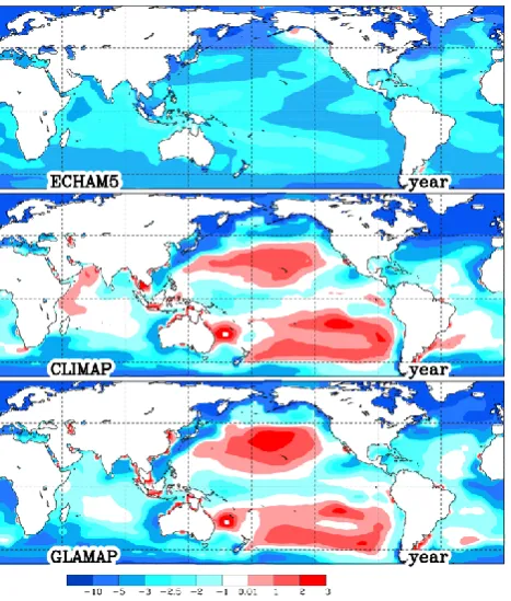
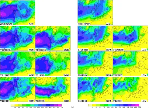
Fig. 1. Annual mean SST differences between the LGM and the
present (NOW). Contours at−10,−5,−3,−2.5,−2,−1,−0.01, 1, 2, 3◦C. Data from the models used here are surface temperatures which over sea ice can become very low.
the chronology. For the latter a set of criteria was defined in order to include or exclude sites to be considered by our analysis. This is discussed in Sect. 4.
2 Description of the simulations
The three LGM simulations available at the Max-Planck In-stitute (MPI) for Meteorology in Hamburg represent differ-ent generations of climatic models and differdiffer-ent resolutions. The simulations have been performed in three different res-olutions (T106, T42, and T31) with the old model version ECHAM3 and the actual model version ECHAM5. The names of the experiments are a combination of the resolution and the model version (T??EH?). Table 1 gives an overview of the naming and conditions for the three sets of simulations. In the old experiments with ECHAM3 (henceforth T42EH3) the SST anomalies including the sea-ice cover were provided by CLIMAP (1981) for the globe but from an inspection (Fig. 1) it seems to be reconstructed only for the northern hemisphere as the SSTs for the LGM differed only slightly from those for the present for the rest of the world, which is hardly realistic. Also, PMIP2 simulations (Braconnot et al., 2007) contained this inconsistency that was confirmed by new tropical SSTs reconstructions from the MARGO project (Kucera et al., 2005). Therefore the
Table 1. SST×resolution atmospheric model.
name SST resolution atmospheric
model
T42EH3 CLIMAP anomalies T42L19–2.8125◦19 levels ECHAM3 T31EH5 coupled T31L19–3.75◦19 levels ECHAM5 T106EH5 T31EH5 anomalies T106L39–1.125◦39 levels ECHAM5
coupled coarse resolution ECHAM5-MPIOM atmosphere ocean model simulations were carried out, though with a very low horizontal resolution of T31 (henceforth T31EH5). In such a coupled model, the atmosphere as well as the ocean and the vegetation were simulated and interact with each other and generated its own SST, sea ice and vegetation pa-rameters. This SST anomalies and sea ice cover was then used for an uncoupled ECHAM5 T106 atmospheric simula-tion (T106EH5).
The models were run on the one hand with the present-day conditions concerning the orography, solar radiation, land ice cover and pre-industrial atmospheric CO2concentrations (280 ppm). On the other hand the models were run under LGM conditions concerning these parameters (atmospheric CO2concentration – 200 ppm for the ECHAM3 simulation, 185 ppm for the ECHAM5 simulations). In the ECHAM5 runs also CH4 has changed from 760 to 350 ppb (ctrl to LGM) and N2O from 270 to 200 ppb. The ECHAM3 sim-ulation was run with SST anomalies and sea ice distributions as reconstructed by CLIMAP (1981). The high-resolution simulations for the present and the LGM with a T106 res-olution (corresponding to approx. 1.125◦ horizontal reso-lution, henceforth T106EH5) model with 39 vertical lev-els were carried out with the ECHAM5 atmospheric model (Roeckner et al., 2003). The boundary conditions, e.g. the SST and vegetation parameters, were taken from the cou-pled ECHAM5-MPIOM atmosphere ocean dynamic vegeta-tion model (Mikolajewicz et al., 2007) simulavegeta-tions, which have been carried out for the present and the LGM with a spectral resolution of T31 (corresponding to approx. 3.75◦) and 19 vertical levels. The experimental setup is largely con-sistent with PMIP2 and some data from these experiments can be found in the PMIP2 data base. For the T106EH5 simulations, these SSTs were corrected for systematic er-rors of the coupled run by adding the SST differences be-tween observed SSTs and simulated ones for the present. The largest correction appeared over the central northern At-lantic, halfway between New York and Madrid, providing warmer values up to 8◦C due to a too zonally simulated Gulf
For defining the topography and the land-sea (L-S) mask, the 5 min data sets from PMIP2 (Peltier, 2004) for 0 ka and 21 ka were interpolated linearly to a T106 grid. For deciding on the L-S mask, at the pixel level of 1/12◦grid, a grid point was called land if the topography was larger than zero. After that the pixels were averaged to the T106 grid. Large lakes were not found by this method. To solve this, for the experi-ment with T106EH5 for the present a standard L-S mask used at MPI was used to incorporate or correct the following lakes: Caspian Sea, Aral Sea, Lake Baikal, some smaller lakes in northern Russia, Lake V¨anern in Sweden, the Great Lakes and some further lakes in Canada, Lake Chad, Lake Victoria and a widening of the Congo River creating one grid point re-garded as a lake. On the other hand, some smaller fjords on the Greenland coast were assumed to be land. Lake Eyre in Australia is, according to the zero-orography criterion, a lake but as it is mostly dry it was assumed to be land. The same criteria have been used for the LGM data set and the result-ing L-S mask was compared with the present-day L-S mask just created. For some northern lakes, the glacier mask uti-lized over-ruled the question of lake or no lake, e.g. for the Great Lakes. For the Black Sea we took the shape as pro-vided by the PMIP2 data using the zero-level criterion. The provided data set did not have a Caspian Sea although large parts of it are deeper than−100 m. A controversial discus-sion about the size of the Caspian Sea and the Black Sea dur-ing the LGM is still godur-ing on (Leroy et al., 2007). It is known that there was a Caspian Sea during LGM. However, it is not known whether it was larger (because of a possible diversion of northward flowing rivers to the south due to glaciers along the Arctic coast or of the Amu-Darya), or smaller (because of a possible drier climate) and therefore, for the LGM sim-ulation, we left it as it is now. The same decision was taken for other lakes.
The coupled ECHAM5-MPIOM atmosphere ocean dy-namic vegetation model (Mikolajewicz et al., 2007) also pro-vided the vegetation parameters for T106EH5. Along the Arctic coast of western Siberia, the glacier data and the land using the zero-orography criterion left a gap which would create two large lakes into which the Ob and Yenisey Rivers would discharge. The glaciers north of it would prevent drainage into the ocean and larger lakes would evolve, which Grosswald called Pur and Mansi Lakes (Grosswald, 1980). Using the PMIP2 data, the water level of these lakes would need to rise at least 170 m before the water could drain into the ocean. This level is used in this study to define such lakes. The interpolation of the SST, sea-ice and vegetation pa-rameters from the T31 resolution of the coupled model sim-ulation to T106, needed for forcing the uncoupled run, was done using bilinear interpolation taking into account land-sea differences. Some grid points, however, needed special con-sideration because of the large difference in resolution which allowed large differences in topographic heights and had a more structured L-S mask in the T106 resolution.
As a criterion for selecting a suitable 25 year period from the 1500 years of simulation with the coupled model, we de-cided to use a period of lowest SST variability to avoid ex-tremes (years 2906–2930 were chosen for the present and the LGM).
As the three models used here differed in several aspects, also standard Atmospheric Model Intercomparison Project (AMIP – Gates, 1992) type simulation data were taken into account. AMIP was designed to investigate the performance of different atmospheric models which were driven by the same external forcings including monthly mean observed SSTs. At MPI such simulations with the ECHAM5 model using a range of different resolutions are available (Roeck-ner, 2003; see also Arpe et al., 2004). From this data set the sole impact of resolution on the model performance can be found. It is referred to below as ROECKNER2003. Ramstein et al. (2007) and Jost et al. (2005) discuss the impacts of res-olution on the model results and find in one regional model a significant increase of precipitation compared to the driving global model. The impact of resolution in our simulations will be discussed in Sects. 3 and 4.
3 Differences between the simulations
The main parameters for plant growth and their survival are thermal and hydrological conditions. Therefore below the focus will be on near-surface air temperatures and precip-itation. For the understanding of the changes and the dif-ferences between the models also some dynamical quanti-ties relevant for the climate of Europe are presented and dis-cussed.
3.1 Sea surface and 2 m air temperatures
K. Arpe et al.: Climate simulations for the last glacial maximum and summer-green tree refugia 95
(a) (b)
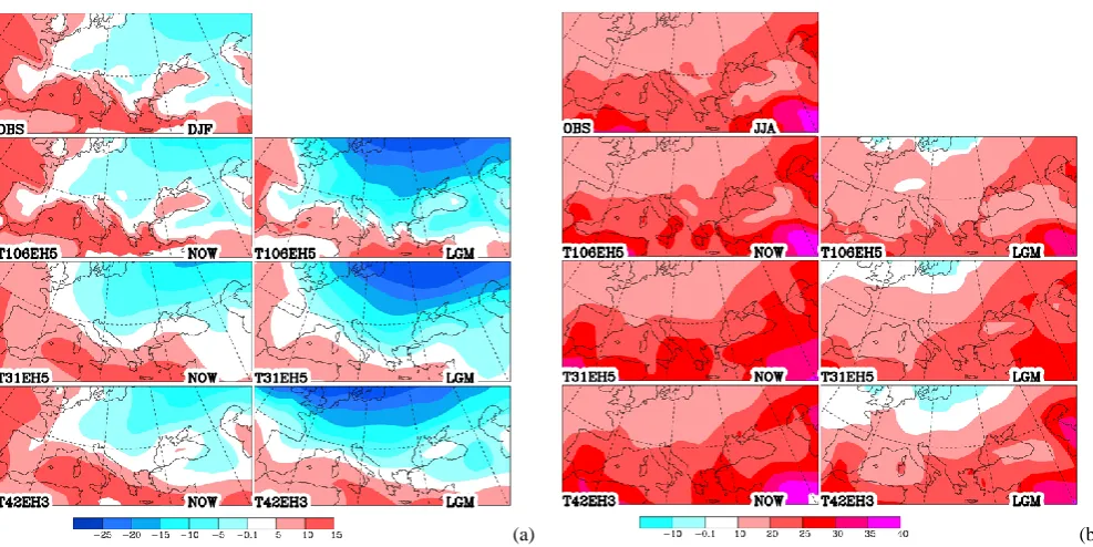
Fig. 2. 2m temperatures for the LGM and NOW as simulated, OBS is the present as analyzed by ERA40 (Uppala et al., 2005), (a) for winter,
contours every 5◦C, down to−25◦C, (b) for summer, contours at−10,−0.1, 10, 20, 25, 30, 35◦C.
than NOW in all simulations, especially in CLIMAP. The CLIMAP simulation for the LGM has much more zonally orientated isotherms and has a very strong gradient over the Atlantic which probably has an impact on the general circu-lation of the atmosphere (see Sect. 3.2).
The differences in the SSTs and sea ice distributions be-tween CLIMAP and the ECHAM5 simulation are in agree-ment with PMIP2 (Braconnot et al., 2007). Otto-Bliesner et al. (2009) further suggest that these new simulations are in general agreement with new tropical SSTs reconstructions from the MARGO project (Kucera et al., 2005). The PMIP2 models give a range of tropical (defined as 15◦S–15◦N) SST cooling of 1.0–2.4◦C, comparable to the MARGO esti-mate of annual cooling of 1.7±1◦C. This fits well with the ECHAM5 simulations, shown in Fig. 1, which were not in-cluded in the PMIP2 runs used by Otto-Bliesner et al. (2009). The PMIP2 models simulate greater SST cooling in the trop-ical Atlantic than in the troptrop-ical Pacific, while the ECHAM5 simulations suggest more cooling for the tropical Pacific.
The consequences of the SST changes for the temper-atures over Europe during winter and summer are shown in Fig. 2 where the 2 m temperatures (2 mT), as simulated for the present (NOW) and LGM and as observed using the European Centre for Medium-Range Weather Forecasts (ECMWF) reanalysis data (OBS), are displayed. Compar-ing the 2 m temperatures of the simulations for the present with the observations shows clearly the best performance of T106EH5, e.g. over western Europe. The differences be-tween the two ECHAM5 simulations are not only due to the
different resolutions but also due to differences in the SSTs, as the T106EH5 SSTs are corrected for a systematic error of the coupled model, as explained above. The up to 8◦C cooler SSTs over the North Atlantic in T31EH5 may have led to cooler 2 mT over Europe compared with T106EH5 for the present and LGM. In winter the cooler North Atlantic SSTs with its implications on sea ice during the LGM in the CLIMAP data generate clearly cooler 2 m temperatures for western Europe while the two ECHAM5 simulations pro-vide cooler temperatures for eastern Europe. From ROECK-NER2003 one can see that the T106 and T31 simulations would look more similar without the SST corrections in the T106 run.
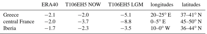
Note the much more structured cooling over the Alps for summer in T106EH5 during the LGM compared to the other runs shown in Fig. 2b. Here the higher resolution of the model which includes as well a better resolution of the orog-raphy shows a direct impact. This turns out to become im-portant in the discussions below. Of further interest for the survival of plants is the temperature variability from year to year. In Table 2 the minimum winter temperature anomalies for three areas in the T106EH5 simulations for the present and the LGM as well as in ERA40 are compared. The in-crease of anomalies during the LGM by a factor of 2 may be an issue as discussed below.
Table 2. Extreme cold 2 m temperature anomalies during winter (DJF) in recent years in the ERA40 analyses and in the T106EH5 simulations
for the present and for the LGM for land points only on a T106 grid.
ERA40 T106EH5 NOW T106EH5 LGM longitudes latitudes
Greece −2.1 −2.0 −5.1 20–25◦E 37–41◦N
central France −2.0 −3.7 −8.8 0–5◦E 45–50◦N
Iberia −1.7 −2.3 −3.5 10–0◦W 36–44◦N
3.2 Atmospheric circulation
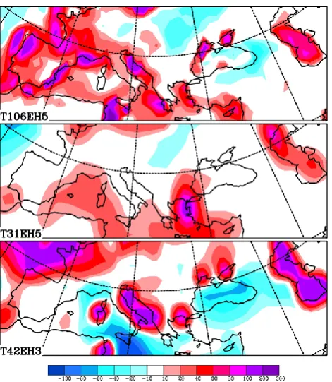
Figure 3 shows the 500 hPa height fields for the present, overlaid in colour are the differences between the LGM and the present. Blue colours indicate that during the LGM the 500 hPa height field was lower than NOW and red vice versa, e.g. for T106EH5 during winter (Fig. 3 left) the Alaskan ridge and the trough over eastern North America were much stronger during the LGM than for NOW. The T31EH5 model shows similar patterns while the simulation with CLIMAP SSTs and their implications on the sea-ice cover is very different: the ridge over western Europe shown for the present is completely wiped out for the LGM. For summer (Fig. 3 right) the changes from NOW to LGM are less pronounced in all simulations. A slight ridging over east-ern Europe during the LGM might be of importance.
In Fig. 4a, the zonal wind for winter (DJF), averaged be-tween 30◦W and 10◦E (eastern Atlantic and western
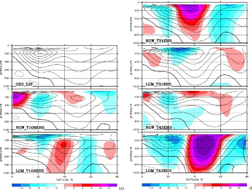
Eu-rope), is shown in height-latitude cross-sections. The up-per panel is the observation as produced by the ECMWF re-analysis (ERA40; Uppala et al., 2005). The lower two panels show the wind as simulated by T106EH5 for the present and the LGM; overlaid in colours are the differences from the field in the panel above, i.e. in the middle panel the colours show the model errors for the present and in the lower panel they show the change between the LGM and the present as simulated by the same model. The T106EH5 simulation for the present has a subtropical jet (20◦N, 200 hPa) which is slightly too weak and stretches too far to the south. The polar jet (50◦N, 300 hPa) is slightly stronger than observed (ERA40).
During the LGM the polar jet is even stronger and 7◦ fur-ther south while a reduction in the westerlies occurs at 60◦N suggesting that the polar jet is forced by the massive ice sheet to go either further south or north of it. This leads to en-hanced precipitation over the Mediterranean Sea during the LGM, shown below. The stronger jet fits in as well with the stronger north-south gradient of surface temperatures shown in Fig. 1. Florineth and Schl¨uchter (2000) suggested from palaeo-data a more southerly position of the main flow dur-ing the LGM over the Alps, supportdur-ing the simulation by the T106EH5 model.
Synoptic meteorologists who analysed weather maps by hand before the existence of numerical weather forecasts used for winter the−30◦C isotherm at the 500 hPa level as
Fig. 3. 500 hPa geopotential height field for the present (heavy
lines) overlaid by the difference LGM-NOW (in colours). Contours for the height field every 8 dam (geopotential decametres), high-lighted lines for 516 and 556 dam in DJF (left) and for 556 and 580 dam in JJA (right). Contours for the differences at±2, 6, 10, 14, 18 dam, blue colours for LGM – NOW values<−2, red>+2.
K. Arpe et al.: Climate simulations for the last glacial maximum and summer-green tree refugia 97
(a) (b)
Fig. 4. Latitude-height cross-section of the zonal wind for winter (DJF) averaged between 30◦W and 10◦E. In the panels for the present (NOW) the differences to the observation are overlaid in colours, i.e. the model error, and in the panels for the LGM simulation the difference to NOW are overlaid in colours. Contours every 5 m s−1, heavy line for the 0-zonal wind contour and dashes for negative values. Red colours for increases by more than 2 m s−1and blue colours for decreases by more than 2 m s−1. (a) Analysis (OBS) and T106EH5 simulation. (b) T31EH5 and T42EH3 simulation.
seasons. No reason why such fixed thresholds should exist is known. If the same thresholds between air-masses exist also for the LGM one would expect a southward shift of the fronts and jets in a generally colder climate. Here it is shown that the model suggest such shifts for the LGM which means that the threshold between air-masses does not change in a colder climate.
A similar but pole-ward shift of the jet streams and the associated fronts and cyclone tracks has been found for the global warming experiments (e.g. Bengtsson et al., 2006) which can be assumed to be due to the same reason as the equator-wards shift in a colder climate shown here. There have been a lot of speculations about the cause of this shift. Quan et al. (2004) verified model results with observational data for the last 50 years. They draw a connection between the shift of the jet and a widening of the Hadley circulation
and found as well an involvement of an ENSO frequency increase. In the T31EH5 simulation in a similar way but with the opposite sign, a decrease of the ENSO frequency was found with an equator-ward shift of the jet for the LGM. However the cause is not fully understood.
with resolution as shown here, which would indicate the in-fluence of the simulated North Atlantic SST error in the cou-pled model. The difference between the LGM and present-day simulation bears, however, some similarities to those of the T106EH5 simulations. The changes from the present to LGM are strongest in the T42EH3 simulations. The polar jet (50◦N, 300 hPa) was already enhanced in T106EH5 for the LGM by more than 2 m s−1compared with the present but in the T42EH3 simulation the increase is more than 25 m s−1, probably due to the much colder SSTs in the northern At-lantic with their implications on the sea-ice cover and warmer tropical SSTs during the LGM in the T42EH3 data compared to the ECHAM5 simulations. Such a stronger north-south SST gradient provides a stronger forcing for the atmospheric circulation. Kageyama et al. (1999), using the same T42EH3 together with other simulations, refer to this enhanced jet stream over the eastern Atlantic as an eastward shift of the jet and found similar shifts in all simulations with the same SST forcing.
LA2007 noticed a massive increase of winter surface wind in the T42EH3 simulations for the LGM over Europe. This can also be seen in the cross-sections of the zonal mean wind at 1000 hPa shown above (Fig. 4b) with increases of 5 m s−1. In this presentation at this level the differences in wind speed for the other simulations were very small, the differences shown by the colours for T106EH5 mainly mean a south-ward shift in the position of the maximum wind. Maps of summer and winter mean surface winds (not shown) demon-strate as well a much lesser increase in wind during winter during the LGM for the two ECHAM5 simulations. Com-mon to all simulations is an increase in the Trade Winds off North Africa in summer and an increase in the North Atlantic westerlies in winter for the LGM, which fits well with the en-hanced meridional temperature gradient.
3.3 Precipitation
Figure 5a shows the winter (DJF) simulated precipitation for the present (NOW) and the LGM. The estimate by GPCP (Huffmann et al., 1996) using observations is also included. All simulations for the present show similar features to those observed. One can, however, easily see that the T106EH5 simulation fits best to the observations. For the LGM, LA2007 have previously pointed out that the cyclone tracks, indicated by the precipitation patterns, take a very different course in the LGM simulations compared with the present, i.e. during the LGM the cyclones in the T42EH3 simulations move from the British Isles straight eastward into Europe in-stead of towards Scandinavia as for the present. In T106EH5 a branch towards Scandinavia can still be seen for the present as well for the LGM though weaker for the LGM and a second branch towards the Mediterranean Sea, somewhat stronger during the LGM reaching Lebanon/Israel/Jordan. This branch is clearly further south than in the T42EH3 sim-ulation for the LGM. The T106EH5 simsim-ulation with higher
precipitation in the Levant is probably realistic as it is known that the Dead Sea had a high stand during the LGM (Stein et al., 2010). The shift of the precipitation towards the Mediter-ranean Sea during the LGM also fits the study by Florineth and Schl¨uchter (2000) who found that the precipitation for the Alpine glaciers had their source to the south of them.
During summer (JJA) for the present (NOW), shown in Fig. 5b, the lower resolution model simulations show less precipitation over the northern Atlantic and northern Europe than the observations while T106EH5 is more realistic. Com-paring the LGM simulations with those for the present, one finds much less aridity for the LGM in the ECHAM5 simula-tions (T106 and coupled T31) for Europe than in the T42EH3 simulations, probably due to the much warmer northern At-lantic SSTs in the ECHAM5 simulations. Over western Europe, T106EH5 provides even more precipitation for the LGM compared with the present which has to be assigned to enhanced evaporation over the northern Atlantic during the LGM (not shown).
The differences between the T106EH5 and T31EH5 are not only due to the different resolutions but could also be in-fluenced by the warmer SSTs in T106EH5 as they had been corrected by the systematic error of the coupled run, as de-scribed above. From ROECKNER2003 one can find that the T106 and the T31 simulations would look more similar with-out the SST corrections in T106EH5 but the impacts from resolution alone are dominant. These changes in the precip-itation over Europe are consistent with the changes in the upper air wind field as discussed above.
Braconnot et al. (2007) compared the precipitation in the PMIP2 coupled model simulations with the uncoupled PMIP1 simulations and found less drying for central and southern Europe in the PMIP2 coupled simulations, even with an increase of precipitation for western Europe dur-ing the LGM in annual means. In annual means for western Europe also the T106EH5 simulation provide an increase in precipitation during the LGM of up to 90 mm season−1(not shown) which is similar to the PMIP2 results. The coupled T31EH5 simulations have an increase of only a third of the T106EH5 values. Jost et al. (2005) also find a clear impact of the model resolution on the precipitation. Higher reso-lution models are able to reproduce the reductions of pre-cipitation found in the palaeo-data more closely than their low-resolution counterparts do; but the simulated climates are still not as arid as reconstructed from palaeo-data. The high-resolution limited area model HadRM even shows in-creases of annual mean precipitation reaching values simi-lar to those of our high-resolution model. ROECKNER2003 data suggest such an increase of precipitation just from the increased resolution.
K. Arpe et al.: Climate simulations for the last glacial maximum and summer-green tree refugia 99
(a) (b)
Fig. 5. Precipitation as estimated for the truth (GPCP; Huffman et al., 1996) and simulated by the models. Contours at 10, 25, 50, 75, 100,
150, 200, 250, 300, 400, 500, 600 mm season−1, (a) for winter, (b) for summer.
3.4 Precipitation minus evaporation
The availability of water for run off and vegetation is best shown by the difference between precipitation and evapora-tion (P−E). In Fig. 6 annual mean differences between LGM and NOW are provided. Because of model constraints, the long-term meanP−Ecannot be negative over land as only water which has fallen can be evaporated. For the lower resolution simulations, some negative numbers along coasts can occur over continents due to interpolations to T106, re-quired for the plotting software which results in less strong gradients along coastal lines in Fig. 6. The general reduction of the precipitation shown above for the LGM is not reflected in theP−Eplots as the evaporation is also reduced during the LGM. Over western Europe including the Iberian Penin-sula P−E is even enhanced in all simulations especially for T106EH5. For Lebanon and Israel in T106EH5 an en-hanced availability of water for the LGM is clearly indicated (for T31EH5 only slightly), in accordance with an observed higher stand of the Dead Sea. The ECHAM5 simulations
show less water availability during the LGM for eastern Eu-rope. If one is interested in intra- or inter-annual variability the best variable to look at would be the soil moisture but its calculation depends on many less well-known quantities.
Fig. 6. Annual mean precipitation minus evaporation (P−E) in the simulations, difference between LGM and NOW. Contours at ±0, 10, 20, 40, 60, 80, 100, 200 mm season−1. Negative values are blue, positive red.
mean precipitation has to be larger or equal to the evapora-tion, therefore no absolute figure can be given.
4 Possible summer-green tree growth during the LGM
So far it has been shown in many examples that the T106EH5 simulation provides the best reproduction of the present cli-mate. Intuitively one may assume that the model which pro-vides best estimates for the present climate would also be best for simulating a climate with a different external forc-ing such as durforc-ing the LGM. Validation is, however, diffi-cult; but some aspects have already been discussed above where the T106EH5 simulation seems to be more realistic, e.g. the more southerly position of the cyclone track over the Mediterranean Sea into the Levant, explaining the high stand of the Dead Sea during LGM, and a southward shift of the polar jet. We use here the method from LA2007 to esti-mate the likeliness of summer-green tree growth during the LGM and compare this with the available pollen, charcoal and fossil wood findings. There, and in this study, a sim-ple down-scaling method is used which partly compensates for systematic errors. For this down-scaling the difference between the simulations for the LGM and for the present is added to a high-resolution climatology of the present (Lee-mans and Cramer, 1991). The resolution of this climatology
Table 3. Minimum requirements for summer-green tree growth
from LA2007 and used in this study.
Parameter cold-tolerant warm-loving
mean temperature of coldest month (◦C) −15 −2.5
GDD5 (day◦C) 800 1000
summer precipitation (mm season−1) 50 60
is 0.5◦corresponding to 55 km in meridional and 40 km in longitudinal direction in the area of interest. The following investigation will be done on this resolution although it is known that observational data on their own do not support such a high-resolution and a danger of over-interpretation of the data exists. Still many local features, which might be im-portant for plant habitats especially in mountainous areas are not resolved by this resolution.
A better model should give possible tree growth at more sites with verified growth. Warm-loving and cold-tolerant summer-green trees are investigated. Typical warm-loving trees in this investigation are: Castanea, Juglans, Platanus, Rhamnus, Fraxinus ornus, Vitis, Quercus pubescens and Os-trya, and cold-tolerant trees are: Carpinus, Corylus, Fagus, Tilia, Frangula, Acer, Populus, Fraxinus excelsior, Alnus, Quercus robur and Ulmus. More details can be found in LA2007
LA2007 used the summer precipitation, the minimum monthly mean 2 m temperature and the growing degree days (above 5◦C) (GDD5) as limiting factors for possible tree
growth. Similarly, for each of these variables and the com-bined score the possible tree growth in the three simulations is investigated. The minimum requirements for growth of these trees are given in Table 3 which is taken from LA2007. 4.1 Palaeosite selection
A few sites have been suggested as possible refugia for trees during the LGM; but those sites without a proof or where the palaeo-data were not properly dated or did not cover the LGM, were not included in our study. Reliable sites had to have a sub-continuous curve of at least one taxon from our list and an age of 21±2 cal Ka BP.
K. Arpe et al.: Climate simulations for the last glacial maximum and summer-green tree refugia 101 is coeval with the lowest stand of sea level (Yokoyama et
al., 2000), avoids all known Heinrich Events in the North Atlantic region, and excludes most of Dansgaard-Oeschger climate event 2 (D/O2), as dated in the GISP2 ice core and in the GRIP core with the chronology of Hammer et al. (1997). This definition (21±2 ka) is used here for simulation valida-tion and for deciding if findings of pollen, charcoal or fossil wood from summer-green trees can be assigned to the LGM or not. Peltier and Fairbanks (2006) suggested recently that the time of maximal glaciation started already 3000 years earlier but this was not taken into account in our investiga-tion.
With these requirements of a site to be called reliable, 24 sites have been identified and are listed in Table 4. 13 ma-rine sites fulfil the requirements as well and are also included in Table 4. However, it is often not clear where the pollen found at marine sites came from, either by river or wind transport. Because of the large source area for the pollen, the number of potential grid points needs to be increased. Only little weight was given to these sites for validation.
At the sites 8, 19, 20 and 35, some pollen occurrences of warm-loving trees have been found but do not have the required sub-continuous curve of at least one taxon. Never-theless we kept them as sites with warm-loving trees, espe-cially those for Greece because they are three nearby sites of the same quality which suggest at least one refugium in the area. For Siles in southern Spain (site 8) the pollen might have been transported from the other nearby sites with warm-loving trees and its inclusion in or absence from our list hardly affects the conclusion of the study.
Most of the sites with identified warm-loving tree reported as well of findings with cold-tolerant trees. In the following all sites with warm-loving trees are assumed to fulfil as well the requirements for cold-tolerant trees to ease the discus-sion.
Other investigations which compare pollen findings dur-ing the LGM with climate model simulations (e.g. Jost et al., 2005) use the spectra in a more complex way, e.g. a regres-sion method. We preferred a more direct approach by which the connections can more easily be seen. In the following we will compare the simulated distributions for precipita-tion, winter and summer temperature (the latter in the form of growing degree days) with the distribution of cold-tolerant and warm-loving summer green trees and the thresholds as-sociated with the occurrence of these tree types.
4.2 Precipitation
Figure 7 shows the precipitation during the LGM for JJA after a simple downscaling to a 0.5◦ grid. The much stronger precipitation over western and central Europe in the T106EH5 simulation, especially compared to T42EH3, has already been shown above. Most observation sites (indicated by markers) lie in areas with green or blue colours (mean-ing more than 50 mm precipitation per season) which are
Fig. 7. Summer precipitation during the LGM down-scaled to a
0.5◦grid. Contours at 25, 50, 75, 100, 150, 200, 250, 300, 400, 500 mm season−1. Sites with observed summer-green tree growth during the LGM are indicated by markers. Circles: only cold-tolerant trees (continental), triangles: cool or warm-loving trees (continental), Xs: only cold-tolerant trees (marine), crosses: cool or warm-loving trees (marine).
sufficient for possible growth of cold-tolerant trees. Warm-loving trees have a requirement of 60 mm season−1 which is hardly different from the 50 mm season−1 in the plots. Sites 22, 23 and 24 in Table 4, the easternmost continental sites, lie in areas which have deficient summer precipitation in all three simulations. Sites 23 (Ghab) and 24 (Urmia) are in areas devoid of summer precipitation in the present cli-mate.
A more detailed investigation (see Tables 5 to 7), however, shows that Gibraltar also has too little precipitation when us-ing the nearest grid point, probably because a 0.5◦ grid is too coarse for capturing the rough topography of this penin-sula. One has to look into the surrounding 1.5◦away to find a grid point with sufficient precipitation. The T106EH5 simu-lation provides most precipitation for the grid point covering Gibraltar. The same argument probably applies as well for site 21, a small Greek island along the Turkish coast, though even 1.5◦away from the site not enough precipitation can be found; again T106EH5 provides most.
Table 4. Reliable continental and marine sites with summer-green tree growth during the LGM from west to east. In column “tree” the
letters W mean warm-loving trees and C cold-tolerant trees. The evidence of tree growth comes mostly from pollen analysis, except sites 4 (Altamira) and 5 (Nerja) which have findings of charcoal, and site 2 (Gibraltar) which has evidence from pollen and fossil wood.
No long lat site seas/ water depth/ author
city/country altitude tree
Group I: reliable continental sites
1 −6.15 43.05 Lago de Ajo N Spain 1570 C Allen et al (1996)
2 −5.30 36.02 Gorham’s cave Gibraltar 0 W + C Carri´on et al. (2008) 3 −4.70 36.80 Bajondillo S Spain 0–80 W + C Cort´es S´anchez et al. (2008)
4 −4.11 43.38 Altamira N Spain 70 C Uzquiano (1992)
5 −3.81 36.75 Nerja S Spain 158 W Aura Tortosa et al. (2002)
6 −3.67 37.00 Padul S Spain 785 C Pons and Reille (1988)
7 −2.66 36.77 San Rafael S Spain 0 W + C Pantale´on-Cano et al. (2003)
8 −2.30 38.24 Siles S Spain 1320 C some W Carri´on (2002)
9 −0.40 42.73 Tramacastilla NE Spain 1640 C Gonz´alez-Samp´eriz et al. (2005)
10 −0.40 42.99 Formigal NE Spain 1585 C IBID
11 3.18 42.04 Laguna Grande N Spain 1510 W + C Ruiz Zapata et al. (2002)
12 8.81 46.00 L. di Origlio Switzerland 416 C Tinner et al. (1999)
13 11.43 45.29 Po valle Italy 19 C Paganelli (1996)
14 11.75 45.27 Lago della Costa Italy, Po 7 C Kaltenrieder et al. (2009)
15 12.83 48.16 Duttendorf Austria 420 C Starnberger et al. (2009)
16 15.60 40.94 L. Monticchio Neaple Italy 1326 C Watts et al. (1996)
17 20.57 48.85 Safarka NE Slovakia 600 C Jankovska and Pokorny (2008)
18 20.80 40.90 L. Ohrid Albania 693 C Wagner et al. (2009)
19 20.91 39.65 Ioannina Greece 470 C some W Tzedakis (1994)
20 22.27 39.50 Xinias Greece 480 C some W Bottema (1979)
21 23.05 39.44 Kopais Greece 95 C Tzedakis (1999); Okuda et al. (2001)
22 26.30 39.10 Lesvos ML01 Lesbos Greece 323 C Margari et al. (2009)
23 36.30 35.07 Ghab NW Syria 240 W + C Niklewski and Van Zeist (1970)
24 45.33 37.75 Urmia BH2 & BH3 NW Iran 1310 C Djamali et al. (2008)
Group II: reliable marine corings
25 −10.33 40.57 MD95-2039 off Portugal −3381 C Roucoux et al. (2005)
26 −10.20 37.77 SU81-18 off Portugal −3135 C Turon et al. (2003)
27 −9.51 37.93 SO75-6KL off Portugal −1281 C Boessenkool et al. (2001) 28 −2.62 36.14 MD95-2043 Alboran Sea −1841 C Fletcher and S´anchez-Go˜ni (2008)
29 3.72 42.82 MD99-2349 Gulf of Lions −126 C Beaudouin et al. (2007)
30 3.87 42.70 MD99-2348 PRGL1-4 Gulf of Lions −296 C Beaudouin et al. (2007)
31 14.49 38.82 KET8003 Tyrrhenian Sea −1900 C Rossignol-Strick and Planchais (1989)
32 14.70 40.47 C106 Tyrrhenian Sea −292 C Buccheri et al. (2002)
33 17.62 41.29 MD90-917 Adriatic Sea −1010 C Combourieu-Nebout et al. (1998)
34 17.91 41.79 IN68-9 Adriatic Sea −1234 C Targarona (1997)
35 24.61 40.09 SL152 N Aegean Sea −978 C some W Kotthoff et al. (2008)
36 25.00 39.26 MNB3 Aegean Sea −800 C Geraga et al. (2010)
37 28.32 42.40 C-2345 W Black Sea −122 C Filipova-Marinova (2003)
Sierra Nevada, to find sufficient precipitation and one would hardly call the simulations a failure for these sites. The same applies for sites 19 and 20 in Greece for warm-loving trees. In the T42EH3 run, these sites have extremely low values at the nearest grid point, even sometimes with negative values which can happen due to the down-scaling method when the change from NOW to LGM in the simulations is larger than the observed precipitation at that point.
K. Arpe et al.: Climate simulations for the last glacial maximum and summer-green tree refugia 103
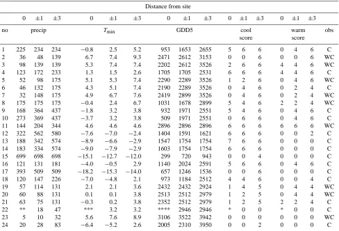
Table 5. Summary of the ECHAM5 T106 run (T106EH5) using JJA precipitation, minimum temperature and growing degree days above
5◦C (GDD5) for continental sites. Values at the nearest grid point of the sites as well as maximum values within a distance±1 or 3 grid points are given for each variable. Unknown values are marked by * because the climatology assumed this point to be water. The category of trees found during the LGM is given by W for warm-loving trees and C for cold-tolerant trees.
Distance from site
0 ±1 ±3 0 ±1 ±3 0 ±1 ±3 0 ±1 ±3 0 ±1 ±3
no precip Tmin GDD5 cool warm obs
score score
1 225 234 234 −0.8 2.5 5.2 953 1653 2655 5 6 6 0 4 6 C
2 36 48 139 6.7 7.4 9.3 2471 2612 3153 0 0 6 0 0 6 WC
3 98 139 139 5.3 7.4 7.4 2202 2612 3526 2 6 6 4 4 6 WC
4 123 172 233 1.3 1.5 2.6 1705 1705 2531 6 6 6 4 4 6 C
5 52 98 175 5.1 5.3 7.4 2290 2289 3526 1 2 6 0 4 6 WC
6 46 132 175 4.3 5.1 7.4 2190 2289 3526 0 4 6 0 2 4 C
7 32 148 175 4.9 6.7 7.6 2419 2899 3526 0 4 6 0 2 4 WC
8 175 175 175 −0.4 2.4 6.7 1031 1678 2899 5 4 6 2 2 4 WC
9 168 364 437 −1.8 3.2 3.8 932 1971 2551 5 4 6 0 4 6 C
10 273 369 437 −3.7 3.2 3.8 509 1971 2551 0 6 6 0 4 6 C
11 144 204 344 4.6 4.6 4.6 2896 2896 2896 6 6 6 6 6 6 WC
12 322 562 580 −7.6 −7.0 −2.4 1404 1591 1621 6 6 6 0 0 2 C
13 188 342 574 −8.9 −6.6 −2.9 1547 1754 1754 7 6 6 0 0 0 C
14 183 334 574 −9.0 −7.9 −2.9 1603 1754 1754 6 6 6 0 0 0 C
15 699 698 698 −15.1 −12.7 −12.0 299 720 943 0 0 4 0 0 0 C
16 121 131 181 −4.0 −0.5 2.9 1140 2024 2591 5 6 6 0 4 6 C
17 393 509 509 −18.2 −15.3 −14.0 657 1246 1536 0 0 6 0 0 0 C
18 120 147 226 −7.0 −4.8 2.1 973 1184 2512 4 4 6 0 0 4 C
19 57 114 131 2.1 2.1 3.6 2432 2432 2924 1 4 5 0 4 4 WC
20 60 88 131 0.1 0.1 3.8 2513 2512 2979 1 2 5 0 4 4 WC
21 63 75 131 −0.3 0.2 3.8 2352 2512 2979 1 2 5 2 2 4 C
22 ** 18 47 *** 3.2 3.2 **** 2946 2946 * 0 0 * 0 0 C
23 5 10 32 5.6 7.6 8.9 3106 3522 3942 0 0 0 0 0 0 WC
24 20 28 83 −6.4 −5.2 2.6 2005 2310 3950 0 0 2 0 0 0 C
difference between the present and the LGM in the T42EH3 simulation was even larger than the observed precipitation leading to negative precipitation values for the T42EH3 run due to the down-scaling method used here. So the wetter Iberian Peninsula in T106EH5 is supported by findings of trees during the LGM.
Also for sites 19–24 the T106EH5 simulation gives high-est precipitation though not reaching the 50 mm season−1 level. Site 24, Urmia, is a lake in a very arid area in north-western Iran. Lake Urmia (or Orumiyeh), is one of the largest permanent hyper saline lakes in the world and resembles the Great Salt Lake in the western USA in many aspects of its morphology, chemistry and sediments (Kelts and Shahrabi, 1986). No tree growth can be found in its surrounding area now. Figure 6 suggests only small changes in available water between NOW and LGM, in fact a small decrease in annual mean available water (P−E) can be found in the T106EH5 and T42EH3 simulations. Therefore one has to assume that the pollen found there have been transported from further
away. The prevailing wind in the ERA40 observation data in May to July, using monthly mean zonal and meridional wind components, is from the east with low wind speeds. This wind is best simulated by the T106EH5 model for the present though with some increase of speed and a slightly more northerly component. The simulation for the LGM hardly differs in this respect from the present. So the source of pollen at Lake Urmia is the coastal area of the Caspian Sea.
Site 23 in Syria is also a very dry area in summer though with sufficient precipitation in spring and winter. Figure 6 suggests some more available water in annual means during the LGM than at the present. At the present time the trees under consideration here could only survive along rivers and it is doubtful that it was much different during the LGM.
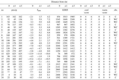
Table 6. Same as Table 5 for the ECHAM5 T31 coupled simulation (T31EH5).
Distance from site
0 ±1 ±3 0 ±1 ±3 0 ±1 ±3 0 ±1 ±3 0 ±1 ±3
no precip Tmin GDD5 cool warm obs
score score
1 163 162 162 −2.1 1.5 4.2 454 1013 1905 0 4 6 0 2 4 C
2 32 45 136 5.1 5.9 7.2 1545 1649 2349 0 0 5 0 0 2 WC
3 94 136 136 3.3 5.9 6.8 1285 1649 2276 2 4 5 2 2 2 WC
4 70 117 153 −0.3 −0.1 1.1 967 967 1852 1 3 6 0 0 4 C
5 46 93 167 3.3 3.3 6.8 1303 1302 2276 0 2 5 0 2 2 WC
6 40 125 167 2.5 3.3 6.8 1235 1302 2276 0 1 4 0 0 2 C
7 26 142 167 3.2 5.2 6.8 1404 1826 2276 0 1 3 0 0 2 WC
8 168 167 167 −2.3 0.4 5.2 559 970 1826 0 2 3 0 0 2 WC
9 111 281 355 −2.8 2.1 2.7 541 1389 1721 0 1 6 0 2 4 C
10 190 281 355 −4.6 2.1 2.7 176 1340 1721 0 2 6 0 0 4 C
11 128 178 293 4.8 4.8 5.3 2392 2391 2391 6 6 6 6 6 6 WC
12 244 477 488 −7.0 −6.5 −2.0 1046 1230 1241 5 5 6 0 0 0 C
13 130 274 497 −6.3 −4.7 0.0 1190 1412 1412 5 5 5 0 0 2 C
14 129 270 497 −5.8 −4.8 0.0 1250 1412 1412 5 5 6 0 0 2 C
15 625 625 625 −13.9 −11.8 −10.0 76 389 572 0 0 0 0 0 0 C
16 98 110 152 −4.5 −1.0 1.9 706 1552 1950 0 3 3 0 2 2 C
17 276 402 402 −15.4 −12.4 −10.5 492 1058 1421 0 4 4 0 0 0 C
18 105 121 195 −8.9 −7.1 −0.1 769 988 2140 0 3 6 0 0 0 C
19 47 109 123 −0.1 −0.1 2.9 1912 1912 2341 0 3 4 0 0 0 WC
20 59 87 123 −1.8 −1.8 2.9 2141 2140 2419 1 2 4 0 0 2 WC
21 64 75 123 −2.7 −1.8 2.9 2005 2140 2419 1 2 4 0 2 2 C
22 ** 19 47 *** 0.4 0.9 **** 2593 2593 * 0 0 * 0 0 C
23 4 10 31 3.3 4.8 6.1 2406 2762 3156 0 0 0 0 0 0 WC
24 22 30 95 −6.3 −5.4 1.4 1592 1832 3229 0 0 2 0 0 0 C
the superiority of the more recent model with their changed boundary conditions.
The three marine sites off Portugal are quite distant from land with sufficient precipitation for tree growth. Naughton et al. (2007) nicely showed that modern samples from marine core tops located SW of Lisbon have similar pollen spectra (more Mediterranean type) as found in the upper part of the Tejo/Tajo river in Spain, i.e. the pollen must have travelled down stream for more than 5 degrees which corresponds to 10 grid-points in our investigation. In this upstream area T106EH5 shows enough precipitation to suggest possible tree growth also for the LGM. Naughton et al. (2007) show as well that the more northern site off Portugal have a pollen spectrum similar to the ones in Galicia, again an area which is further than 3◦away from the site and which show enough summer precipitation for tree growth in the climate simula-tions by all three models.
4.3 Temperatures of coldest month
A further limiting factor for summer-green tree growth is the minimum monthly mean temperature. Earlier it has been
shown that the T42EH3 simulation is quite different in this respect, cooler in western and warmer in eastern Europe, compared with the two ECHAM5 simulations, probably due to its much colder North Atlantic. This can be seen in Fig. 8, the down-scaled presentation, as well as in Fig. 5b, especially over eastern Europe and Turkey. The T106EH5 simulation shows warmer temperatures for Iberia and NW Africa than the T31EH3 simulations. Again ROECKNER2003 suggests that the difference between the two runs is due to the warmer SSTs in the North Atlantic in the T106EH5 simulation. For most of Iberia one finds observation sites in the white or red areas (>−2.5◦C) more so in the T106EH5 simulation,
i.e. areas with possible growth of warm-loving trees. The exception is at the grid point of site 10 (Spanish Pyrenees) where also only cold-tolerant trees have been found. The same applies for the T42EH3 simulation at sites 4, 9 and 10. The temperature of the coldest month does not suggest supe-riority for any of the simulations for western Europe.
K. Arpe et al.: Climate simulations for the last glacial maximum and summer-green tree refugia 105
Fig. 8. 2 m temperature of the coldest month. Contours at±0, 2.5, 5, 10, 15◦C. Sites with observed summer-green tree growth during the LGM are indicated by markers. Circles: only cold-tolerant trees (continental), triangles: cool or warm-loving trees (continental), Xs: only cold-tolerant trees (marine), crosses: cool or warm-loving trees (marine).
a nearby coring in the Venice Lagoon (Canali et al., 2007) shows findings of Ostrya, a warm-loving tree, and cores cov-ering the LGM in the Venetian Po Plain show poorly doc-umented occurrences of Castanea sativa type (Miola et al., 2006). These sites have not been included in our list of re-liable sites because they do not meet our requirements for being categorised as reliable sites. They are mentioned here because these two sites do not agree with the simulated cli-mate. In Fig. 2a it could be seen that the winter tempera-ture difference between NOW and LGM is much more pro-nounced over and around the Alps in the T106EH5 simula-tion compared with the others. This can be assigned to the different representation of the Alps and the Adriatic Sea in the different resolutions of the models. LA2007 showed in their Fig. 1 a better representation of the Alps in a T106EH5 model though with a southward shift of the Po Valley, while the other resolutions did not have a Po Valley at all. This and a resolved Adriatic Sea creates a much warmer (more realistic) winter temperature for the present in the T106EH5 simulation than in the lower resolution models. As the down-scaling method uses only the difference between LGM and NOW from the simulation, it results in cooler temperatures during the LGM in Fig. 8 for the Po Valley in the T106EH5 simulation.
At the grid points of the two sites 15 and 17 in Austria and Slovakia, only the T106EH5 simulation has values be-low−15◦C (less cold in the other two simulations), which
does not agree with the findings of trees there. The other simulations fail at these stations because of the growing de-gree days criterion (see below). The largest differences be-tween the models are at site 17 with temperatures of−18.2 (T106EH5) versus−13.5◦C (T42EH3). Perhaps these sites lie in areas with a local climate which is not resolved by the present data and a higher resolution climatology model might alter this finding. Using the Peltier (2004) orographic data on a 5 min grid, one finds a variation between minimum and maximum heights on a 1◦grid from 127 to 1308 m; though the mean for a 0.5◦grid, the one used here for the climatol-ogy (Leemans and Cramer, 1991), has a height of 555 m near to the one at the site of pollen findings during the LGM. A range of heights of 127 to 1318 m corresponds to a temper-ature range of 8.8◦C when applying a standard atmospheric
lapse rate. Also the slope aspect of the terrain to the north or south would be important in such strongly orographically structured area and the trees may have grown on the south facing slopes.
At several sites across Europe, Peyron et al. (1998) es-timated the coldest mean temperature and annual mean precipitation by grouping pollen taxa into plant functional types (PFTs). These reflect the vegetation in terms of biomes which have a wider distribution than a species. For the present-day, one can provide a range of minimum temper-atures and precipitation in which such PFTs can grow. As the same PFTs can also be found during the LGM, it allows the estimation of ranges of minimum temperatures and pre-cipitation during the LGM. Some of their sites are the same as those used in this study, i.e. sites 6, 16, 19, 20 and 23 (Table 4). At these sites the minimum temperatures given in this study are much warmer than those suggested by Peyron et al. (1998). This suggests for the two Greek sites (19 and 20) that warm-loving trees could not have grown according to the PFT method although some pollen grains have been found there. They also provide annual mean precipitation estimates at these sites which are much lower than those pro-vided by all three model simulations (not shown). More re-cently Wu et al. (2007) could show that the impact of lower CO2 on pollen production during the LGM was not taken care of in earlier estimates. Their new estimates of temper-ature from pollen findings brought a better agreement to the climate based on model simulations of the LGM (Ramstein et al., 2007). Still the new estimates of the temperature of the coldest month in their studies are up to 5◦C cooler than in
the present study. They show also the range of uncertainty in their estimate which is larger than 5◦C. As there is not such a discrepancy between palaeo-data and model simulations in the present study we did not follow up this comparison any further.
Table 7. Same as Table 5 for the ECHAM5 T31 coupled simulation (T31EH5).
Distance from site
0 ±1 ±3 0 ±1 ±3 0 ±1 ±3 0 ±1 ±3 0 ±1 ±3
no precip Tmin GDD5 cool warm obs
score score
1 112 112 127 −5.6 −1.5 1.8 869 1464 1809 2 3 4 0 2 4 C
2 17 27 124 7.1 8.2 8.9 2899 3165 3858 0 0 6 0 0 6 WC
3 73 120 124 6.1 8.2 9.9 2763 3165 3963 1 6 6 2 6 6 WC
4 −6 38 67 −3.4 −3.1 0.9 1583 1583 2699 0 0 1 0 0 2 C
5 20 72 127 6.3 6.3 9.9 2809 2809 3963 0 1 6 0 2 6 WC
6 9 90 127 5.8 6.3 9.9 2665 2809 3963 0 2 6 0 2 6 C
7 −15 100 127 6.8 8.8 9.9 2900 3309 3963 0 4 5 0 2 4 WC
8 127 127 127 1.2 3.7 8.8 1459 2115 3309 5 5 5 2 2 4 WC
9 18 181 253 −4.0 0.9 0.9 1126 2051 2367 0 0 6 0 0 4 C
10 92 181 253 −7.1 0.4 0.9 686 2051 2367 0 6 6 0 0 4 C
11 90 121 219 4.3 4.3 4.6 2553 2552 2552 2 6 6 4 6 6 WC
12 125 344 367 −7.8 −7.3 −2.3 1517 1695 1782 6 6 6 0 0 2 C
13 46 171 395 −6.6 −4.9 0.2 1758 2045 2045 0 6 6 0 0 4 C
14 48 170 395 −6.3 −5.2 0.2 1827 2045 2087 0 6 6 0 0 4 C
15 543 542 542 −15.3 −12.7 −10.6 97 461 968 0 0 4 0 0 0 C
16 78 89 129 −3.1 0.5 3.6 1303 2269 2822 2 2 4 0 4 4 C
17 275 397 397 −13.5 −10.4 −8.0 157 674 1118 0 0 3 0 0 0 C
18 52 68 122 −6.1 −4.7 2.6 1393 1539 2715 1 1 3 0 0 0 C
19 13 69 74 2.6 2.6 6.2 2569 2568 3010 0 1 1 0 0 2 WC
20 28 62 76 1.1 1.1 6.2 2715 2715 3010 0 1 2 0 2 2 WC
21 34 50 76 0.7 1.1 6.2 2545 2715 3010 0 1 2 0 0 2 C
22 ** 5 25 *** 5.4 5.7 **** 3006 3006 * 0 0 * 0 0 C
23 3 8 29 6.0 8.1 9.6 3226 3626 4019 0 0 0 0 0 0 WC
24 13 22 54 −4.8 −3.6 3.2 2203 2466 4051 0 0 1 0 0 0 C
minimum temperature are more realistic in the one or the other simulation. Also the estimates by Wu et al. (2007) do not help in this respect.
Kageyama et al. (2006) noticed in the PMIP2 model sim-ulations for Europe during the LGM a significantly higher inter-annual variability in coldest-month temperatures com-pared to the control runs which means that trees could die already at a warmer mean temperature during extreme years. Our simulations also show an increase of variability of the 2 m winter temperature, stronger e.g. for central France than Iberia or Greece. We are not sure about its significance as there would be more snow during the LGM than NOW and more for central France than Iberia or Greece. Such an increase of snow cover results into a much stronger drop of temperature during nights in winter. More relevant for the survival of trees is the temperature within the top few centimeters of the soil and also there the temperature vari-ability is increased during the LGM. In central France the amplitude of January temperature increases from about 3 to 5.5, for Iberia from 1.5 to 3.5 and for Greece from 1 to 2◦C. Absolute winter minima anomalies of single years for the T106EH5 simulations as well as for the ERA40 data
are given in Table 2. Above we have required for cold-tolerant tree growth a minimum mean temperature of more than−15◦C. Perhaps one should raise this limit by the in-creased amplitude of temperature variability.
4.4 Growing degree days
K. Arpe et al.: Climate simulations for the last glacial maximum and summer-green tree refugia 107
Fig. 9. Growing degree days above 5◦C. Contours at 600, 800, 1000, 1200, 1500, 2000, 8000. Sites with observed tree growth during the LGM are indicated by markers as in Fig. 7.
GDD5 turns out to be a more stringent criterion than the temperature of the coldest month, probably because it repre-sents the growing season while the temperature of the coldest month represents the dormant season and might be responsi-ble for killing the trees when a threshold is passed.
Warm-loving trees need at least 1000 GGD5 which is eas-ily surpassed at all sites with findings of warm-loving trees. 4.5 Summary for summer-green tree growth during the
LGM
Possible growth of summer-green trees is found in a belt be-tween too cold temperatures in the north and too low sum-mer precipitation in the south. The topographic impact can clearly be seen as mountains are often connected with en-hanced precipitation but also with reduced temperatures. As the limits given by the precipitation are similar for warm and cold-tolerant trees, i.e. 50 mm for cold-tolerant and 60 mm for warm-loving trees, the southern limits for both sorts of trees are very similar. The GDD5 and the minimum temper-atures are somewhat complementary but slightly more sites fail on the growing degree days criterion.
In Fig. 10, all limiting factors are taken together. In green or blue coloured areas (values>1) at least the minimum requirements for all parameters are fulfilled, i.e. for cold-tolerant trees there is more than 50 mm summer precipitation,
temperatures of the coldest month are higher than −15◦C
and the GDD5 values are larger than 800 (60 mm,−2.5◦C
and 1000 respectively for warm loving trees). Further away from these minimal requirements higher values are given (up to 7) for possible tree growth (darker colours). The T106EH5 simulation produces larger areas of possible tree growth than the other simulations for western Europe while the T42EH3 run suggests more tree growth in eastern Europe, especially north of the Crimea.
Unfortunately no sites with palaeo-data have been found in these areas with larger differences, France and Ukraine. The detailed contributions from the limiting factors have al-ready been discussed above and only for Spain and Greece a clear advantage for the T106EH5 simulation was shown. The visual impression from Fig. 10a also suggests an advan-tage for the ECHAM5 simulations at Duttendorf in Austria and Safarka in Slovakia, though the detailed numbers do not confirm it for the grid points next to the sites.
In Fig. 10b one can find two interesting shifts for the warm-loving trees at the eastern coast of the Black Sea and the south-western coast of the Caspian Sea with the different simulations. The likeliness of warm-loving summer-green trees moves from the Black to the Caspian Sea from the T42EH3 to the T106EH5 simulation which is due to a shift in the minimum temperature. But the shift is very small.
Tables 5 to 8 provide the detailed values for each site and have already been used in the discussions above. The val-ues in the neighbourhood of the sites in these tables are the maximum values within±1 or 3 grid points calculated for each variable separately. This leads for example in Table 6 for T31EH5 at site 7 to the discrepancy that at±1 grid point all single variables suggest possible warm-loving tree growth but not the combined score, as the grid point with sufficient precipitation is different to the grid point with warm enough temperatures. For the marine sites in Table 8 only values for
±3 grid points are given, as these sites were also mostly sub-merged during the LGM, and pollen must have been trans-ported from further away. The findings by Naughton et al. (2007) suggest even a transport by rivers over distances of 10 grid points for the sites off Portugal. Therefore the marine sites suggest possible tree growth in Galicia and the upper Tejo/Tajo River where especially the T106EH5 simu-lation show suitable climate conditions.
Table 8. Summary of all simulations for marine sites using JJA precipitation, minimum temperature (Tmin) and growing degree days above 5◦C (GDD5). Only maximum values within a distance±3 grid points are given for each variable.
site T106EH5 T31EH5 T42EH3
score score score tree
No prec Tmin GGD5 C W prec Tmin GGD5 C W prec Tmin GGD5 C W obs
25 37 7.8 2420 0 0 30 5.7 1508 0 0 16 5.6 1895 0 0 C
26 41 8.2 2573 0 0 33 6.0 1591 0 0 18 6.7 2077 0 0 C
27 41 8.2 2573 0 0 33 6.0 1591 0 0 20 6.7 2077 0 0 C
28 148 7.8 3526 4 2 142 6.8 2276 1 0 100 9.9 3963 4 2 C
29 344 4.6 2896 6 6 293 5.3 2391 6 6 219 4.6 2552 6 6 C
30 293 4.6 2896 6 6 253 4.8 2391 6 6 187 4.3 2552 6 6 C
31 31 5.1 901 4 4 110 3.8 2074 1 2 89 6.9 3298 2 0 C
32 181 3.1 2378 6 6 152 2.4 1694 3 2 129 4.0 2448 4 4 C
33 238 2.9 2617 6 6 185 1.3 1950 4 4 118 3.4 2822 3 2 C
34 291 2.9 2617 6 6 225 0.8 1950 6 4 151 1.9 2822 4 2 C
35 134 3.7 2964 5 4 132 0.2 2398 5 2 91 4.0 2872 2 2 WC
36 89 3.8 2979 2 4 95 1.2 2419 2 2 76 4.5 2883 2 2 C
37 160 −5.1 2108 6 0 147 −6.3 2121 6 0 84 1.8 2371 2 0 C
(a) (b)
Fig. 10. Possible tree growth during the LGM in the different model simulations combining the summer precipitation, minimum temperature
and growing degree days. For values of 1 and higher (green to blue colours) the minimum requirements for possible tree growth are met, higher values mean more summer precipitation and higher GDD5. Sites with observed tree growth during the LGM are indicated by markers as in Fig. 7. (a) Cold-tolerant trees, sites with warm-loving trees mostly have evidence of cold-tolerant trees as well. (b) Warm-loving trees.
suffers, however, from the uncertainties in the pollen findings at these three sites, as discussed above. All simulations failed to simulate possible tree growth for Urmia in Iran. We as-sume that the pollen found there has been blown from the
coastal area of the Caspian Sea with the prevailing easterly winds in spring and early summer.
K. Arpe et al.: Climate simulations for the last glacial maximum and summer-green tree refugia 109
Table 9. Number of continental sites with observed tree growth
where the simulations suggest possible tree growth at the grid point nearest to the site (0), within±1 grid point, and within±3 grid points (±1.5◦) from the site.
cold-tolerant trees
obs. T106EH5 T31EH5 T42EH3
0 ±1 ±3 0 ±1 ±3 0 ±1 ±3 24 15 18 22 8 19 21 7 16 22
warm-loving trees
obs. T106EH5 T31EH5 T42EH3
0 ±1 ±3 0 ±1 ±3 0 ±1 ±3
9 3 7 8 2 3 7 3 6 8
a range of tolerance from which one could use also a lower value than the 50 or 60 mm season−1applied here. For cold-tolerant trees at the nearest grid point for T106EH5 from the nine failures, six are due to precipitation. For the warm-loving trees a slight disadvantage exists for T31EH5.
Some genetic studies have postulated formerly unknown refugial areas by pointing to locations with a high genetic diversity, for example Crimea (Comes and Kadereit, 1998). Cordova (2007) and Cordova and Lehmann (2006) suggested that the Crimean coast was a refugium for Alnus, Carpi-nus, Corylus, Quercus and Ulmus, i.e. cold-tolerant summer-green trees. Their pollen data did not go as far back as the LGM but, as their earliest data at 12 000 radiocarbon years BP showed pollen from these trees, it is likely that these trees survived the LGM locally. Tsereteli et al. (1982) found pollen of warm-loving and cold-tolerant summer-green trees for the LGM in sufficient numbers to suggest that they were growing locally in Apiancha, Georgia (P. Tarasov, personl communication, 2007). Also their data record did not cover the LGM and therefore both sites are not included in our list of reliable sites; however, both sites are suggested by the model simulations as possible refugia for cold-tolerant trees. Apiancha becomes just too cold for warm-loving trees in the T106EH5 simulation, which is not contradictory to the find-ing of such trees there as these findfind-ings stem from a period before the LGM.
At some sites the simulations suggest the existence of warm-loving trees while the palaeo-data report only cold-tolerant trees. Partly this is due to the fact that some Quercus species are warm-loving while others are cold-tolerant and if in doubt we put the palaeo-data in the cold-tolerant cate-gory. Furthermore pollen analysis has the deficiency that if one does not find pollen, it does not mean that there were no trees, especially during the LGM since the low CO2caused a lower pollen production (Willis et al., 2000; Leroy, 2007; Wu et al., 2007). However, the opposite is valid, though not always valid for the site itself due to possible long-distance transport of the pollen.
Iberia turned out to be an important area for tree refugia because of its higher summer precipitation especially in the T106EH5 simulation compared to the present and still with warm enough winter temperatures. Quite a few sites, also the marine sites off Portugal, with findings of tree pollen or charcoal confirm this model result. This has already been suggested by Gonz´alez-Samp´eriz et al. (2011) on the basis of palaeo-data.
For down-scaling we have used a method in which the dif-ference between the LGM and present-day simulations are added to a high-resolution present-day climatology. Another method applicable mainly for precipitation is to multiply the ratio of LGM over present-day simulation values with a present-day climatology. This method has the advantage that it will not give any negative values for precipitation. If the simulation of the present-day is perfect, the two methods should give the same result. For the T106EH5 simulations this method gives only slight changes with slightly higher precipitation over Iberia and slightly lower precipitation for parts of eastern Europe. For Iberia it means that all sites in Iberia, including Gibraltar, would have received enough summer precipitation to allow the growth of trees while the values for the other sites hardly differ. The other two simula-tions are much more affected; they lose possible tree growth for Italy, Greece and the Caucasus area. The T42EH3 run is the most affected with a loss of most areas with possible tree growth. For consistency (using the same method for pre-cipitation and 2 m temperature) and being comparable with LA2007, we did not use this method.
One of the limitations of the approach followed in this pa-per remains the spatial resolution. Our down-scaling method has reached its limit of possible application as a climatology on a 0.5◦grid used here has a resolution which is higher than
justified by observational data alone. The future will go for higher resolution models, nested or global as done by Sven-ning et al. (2008).