https://doi.org/10.5194/tc-12-2175-2018
© Author(s) 2018. This work is distributed under the Creative Commons Attribution 4.0 License.
Glacio-hydrological melt and run-off modelling: application of a
limits of acceptability framework for model comparison and
selection
Jonathan D. Mackay1,2, Nicholas E. Barrand1, David M. Hannah1, Stefan Krause1, Christopher R. Jackson2, Jez Everest3, and Guðfinna Aðalgeirsdóttir4
1School of Geography, Earth and Environmental Sciences, University of Birmingham, Edgbaston, Birmingham, B15 2TT, UK 2British Geological Survey, Environmental Science Centre, Keyworth, Nottingham, NG12 5GG, UK
3British Geological Survey, Lyell Centre, Research Avenue South, Edinburgh, EH14 4AS, UK 4Institute of Earth Sciences, University of Iceland, 101 Reykjavík, Iceland
Correspondence:Jonathan D. Mackay ([email protected]) Received: 30 November 2017 – Discussion started: 18 January 2018 Revised: 30 April 2018 – Accepted: 18 June 2018 – Published: 6 July 2018
Abstract. Glacio-hydrological models (GHMs) allow us to develop an understanding of how future climate change will affect river flow regimes in glaciated watersheds. A variety of simplified GHM structures and parameterisations exist, yet the performance of these are rarely quantified at the process level or with metrics beyond global summary statistics. A fuller understanding of the deficiencies in competing model structures and parameterisations and the ability of models to simulate physical processes require performance metrics util-ising the full range of uncertainty information within input observations. Here, the glacio-hydrological characteristics of the Virkisá River basin in southern Iceland are characterised using 33 signatures derived from observations of ice melt, snow coverage and river discharge. The uncertainty of each set of observations is harnessed to define the limits of accept-ability (LOA), a set of criteria used to objectively evaluate the acceptability of different GHM structures and parameter-isations. This framework is used to compare and diagnose deficiencies in three melt and three run-off-routing model structures. Increased model complexity is shown to improve acceptability when evaluated against specific signatures but does not always result in better consistency across all sig-natures, emphasising the difficulty in appropriate model se-lection and the need for multi-model prediction approaches to account for model selection uncertainty. Melt and run-off-routing structures demonstrate a hierarchy of influence on river discharge signatures with melt model structure hav-ing the most influence on discharge hydrograph seasonality
and run-off-routing structure on shorter-timescale discharge events. None of the tested GHM structural configurations re-turned acceptable simulations across the full population of signatures. The framework outlined here provides a com-prehensive and rigorous assessment tool for evaluating the acceptability of different GHM process hypotheses. Future melt and run-off model forecasts should seek to diagnose structural model deficiencies and evaluate diagnostic signa-tures of system behaviour using a LOA framework.
1 Introduction
(structure) and numerical constants (parameterisation) is not known. Physically based models which solve equations de-rived from first principles, typically over a distributed grid, are our closest approximation of the “true” structure. How-ever, limited parameterisation data and computer resources often preclude the use of such complex models, particularly in remote mountainous regions where data are scarce and where the inclusion of extra complexity does not guarantee better predictions (e.g. Gabbi et al., 2014).
Simplified process models offer an alternative. They are faster to run and employ fewer parameters, which are typi-cally calibrated to available observation data. They are based on, but do not necessarily adhere to, physical laws and as such their mathematical structure is somewhat unconstrained and may be biased towards a particular scientist’s own per-ceptions and understanding of environmental processes. This has led to the development of a variety of competing model structures which purport to simulate the same process, but which have been derived from different process hypotheses. For example, a number of simplified index model structures of snowmelt and ice melt exist. The classical temperature in-dex model (TIM) simulates melt as a linear piecewise func-tion of temperature only (Braithwaite, 1995), a hypothesis that can be justified because of the influence temperature has on the total energy balance of ice and snow, particularly in temperate climates (Ohmura, 2001; Guðmundsson et al., 2009; Aðalgeirsdóttir et al., 2011). So-called “enhanced” TIM structures have also been proposed, which include added levels of complexity with the purpose of providing more accurate estimates of melt. These have accounted for perturbations in melt caused by topographic shading (Hock, 1999), surface albedo characteristics (Oerlemans, 2001; Pel-licciotti et al., 2005) and debris cover (Carenzo et al., 2016). Similarly a number of simplified representations of pro-cesses governing the hydrological water balance have been used in GHMs. Arguably, the equations that govern the rout-ing (transport) of run-off are most important in relation to river flow predictions in glaciated river basins, as storage characteristics of ice and snow strongly influence river flow regimes over a range of timescales (Jansson et al., 2003). The concept of linear reservoirs is the most widely adopted simplified approach for run-off-routing in glaciated basins (Zhang et al., 2015; Hanzer et al., 2016; Gao et al., 2017). A linear reservoir lumps all of the interacting, non-linear and non-stationary components of water transmission within a predefined area (e.g. a watershed) into a single “leaky bucket”. Despite its simplicity, the linear reservoir has been shown to be remarkably versatile at capturing the storage– discharge characteristics of glaciated river basins around the world (Hock and Jansson, 2005; de Woul et al., 2006; Farinotti et al., 2012). This is partly because the concept lends itself to structural modifications that can represent dif-ferent glacio-hydrological systems. Hanzer et al. (2016) hy-pothesised that the snowpack, firn layer, glacier ice and the region free from ice all exhibit unique run-off-discharge
re-sponses and advocate the use of four linear reservoirs in parallel to distinguish between these units. However, sim-pler structural configurations use only two linear reservoirs in parallel to route meltwater through the snowpack and ice separately (Hannah and Gurnell, 2001) or even a single lin-ear reservoir to route all rainfall and melt run-off simultane-ously (Boscarello et al., 2014), which can accurately repro-duce river discharge time series.
The availability of multiple, presumably plausible, sim-plified model structures presents somewhat of a dilemma to glaciologists and hydrologists as they are left with some uncertainty about how processes should be represented in their models. For the purpose of river discharge predictions, this problem is particularly pertinent, as there are competing structures for two fundamental controls on these predictions: snowmelt and ice melt and run-off-routing. One approach to mitigate this is to determine the optimum structure that best captures the observation data. Structural optimisation of simplified run-off-routing routines has largely been ig-nored in glacio-hydrological contexts (see Hannah and Gur-nell, 2001, for one notable exception), but more studies have sought to optimise and compare simplified models of melt. Gabbi et al. (2014) applied four different TIMs to Rhone-gletscher, Switzerland. They found that all achieved a similar goodness-of-fit to 6 years of ablation stake data, but that the inclusion of a solar radiation term provided the most accurate predictions of multi-decadal measurements of ice volume change. Irvine-Fynn et al. (2014) applied six different TIMs to the high-Arctic Midtre Lovénbreen glacier but only found minor improvements in capturing seasonal ablation stake data when various levels of complexity were introduced to the classical (temperature-only) TIM. More recently, a com-parison of four TIMs applied to four glaciers in the French Alps by Reveillet et al. (2017) found no clear evidence that using an enhanced TIM over the classical temperature-only approach provided better simulations when compared to a 17-year data set of ablation stake measurements. Mosier et al. (2016) used a multi-criterion evaluation approach to compare the performance of different conceptual melt model struc-tures. They compared seven competing melt model structures in two glaciated catchments in Alaska to ablation stake, river discharge and remotely sensed snow coverage data. They found that no single model was best across all of the obser-vation data sets, but the inclusion of a cold-content represen-tation of snow consistently produced the best goodness-of-fit scores over the evaluation data.
the data (Beven, 2016). Beven (2006) argues that, because of this uncertainty and because of the fact that all models are by definition imperfect, no one optimum model struc-ture (or parameterisation) exists. Instead, there is an equi-finality of behavioural models that make predictions within some predefined acceptability bounds around the observa-tion data that take various sources of modelling uncertainty into account. Indeed, parameter equifinality is a well recog-nised phenomenon in conceptual models of snowmelt and ice melt (Jost et al., 2012; Pellicciotti et al., 2012; Gabbi et al., 2014; Finger et al., 2015; Reveillet et al., 2017). If we accept this, then the priority within the glacio-hydrological mod-elling community should be to establish frameworks that al-low us to robustly evaluate model appropriateness and distin-guish between behavioural (acceptable) and non-behavioural (unacceptable) structures and parameterisations. Constrain-ing the range of acceptable models is particularly important for glacio-hydrological modelling, as it has been shown that model uncertainty can lead to high uncertainty in 21st cen-tury predictions of river flows in glaciated basins (Huss et al., 2014).
One potential source of inspiration is the hydrological rainfall-run-off modelling community. Their heavy reliance on an ever-expanding choice of conceptual hydrological pro-cess models to predict river flow prompted Gupta et al. (2008) to discuss the need for a better framework with which to discriminate between these competing process hypotheses. They focussed on the evaluation metrics and noted that there was an overreliance on metrics that quantify the average per-formance of a model (e.g. root mean squared error and Nash– Sutcliffe efficiency), which reduces information held in ob-servation data down to a single summary statistic. They argue for a multi-criterion, diagnostic approach for which more of the relevant information from observation data is extracted so that inadequacies in model structures and parameterisations can be better identified. Rye et al. (2012) applied such an ap-proach to optimise a distributed surface mass balance model of two glaciers in Svalbard. They used ablation stake data to define three different features of the observations including mass balance at the stake locations, long-term mass balance trend and mass balance gradient. Using a multi-objective op-timisation procedure, they identified structural inadequacies relating to how the mass balance gradient was simulated.
Hydrologists are now moving away from traditional met-rics of model performance in favour of more diagnostic sig-natures of hydrological behaviour. These have typically been derived from river flow time series and may be as simple as the mean flow (an indicator of water balance) or they can be used to characterise the distribution (e.g. flow per-centiles) and the timing (e.g. autocorrelation) of flows. They have shown to have more discrimination power than tradi-tional error metrics (Euser et al., 2013; Hrachowitz et al., 2014; Shafii and Tolson, 2015; Schaefli, 2016) and, impor-tantly, it is also possible to take into account their informa-tion content (i.e. their uncertainty) so that decisions about
model appropriateness can be made within the uncertainties of observation data used to evaluate the model. Here, obser-vation data uncertainty can be used to define quantitative lim-its of acceptability (LOA) around each signature. Different model structures and parameterisations can then be system-atically evaluated for their ability to capture the signatures within their LOA, allowing the modeller to objectively di-agnose model deficiencies and make decisions about model appropriateness. The LOA framework has been used to con-strain the parameters of a distributed hydrological model for flood prediction (Blazkova and Beven, 2009), evaluate the appropriateness of different hydrological model structures across contrasting geological settings (Coxon et al., 2014) and, most recently, to diagnose deficiencies in a hydrological model based on its ability to capture a range of river dis-charge signatures for an alpine catchment (Schaefli, 2016).
run-off-routing model structures across the range of signa-tures.
2 Methodology 2.1 Study site
The Virkisá River basin covers an area of 22 km2 on the western side of the ice-capped Öræfajökull stratovolcano in south-eastern Iceland (Fig. 1). It rises from near sea level to the west, where it is bounded by steep cliffs, up to an ice-filled caldera at the summit of Öræfajökull (∼2000 m a.s.l.), the edge of which forms the basin’s uppermost boundary. The basin forms a major drainage channel for accumulated ice which flows in a south-westerly direction down the steeply sloped Öræfajökull (average slope of 0.25). It flows along two distinct glacier arms (Virkisjökull and Falljökull, here-after referred to as Virkisjökull), around a bedrock ridge before meeting again at the terminus (∼150 m a.s.l.). Virk-isjökull has a high mass balance gradient with a net an-nual accumulation of more than 7 m w.e. yr−1 at the sum-mit (Guðmundsson, 2000) and net annual ice melt of more than 8 m w.e. yr−1in the main ablation zone (Flett, 2016). It has been in a phase of retreat since 1990 due to warming of the climate over this period (Hannesdóttir et al., 2015). Since 2005 the rate of retreat has accelerated to>30 m yr−1as a re-sult of the detachment of the ice front from the active part of the glacier, resulting in rapid downwasting (Bradwell et al., 2013; Phillips et al., 2014; IGS, 2017). This recent rapid re-treat has resulted in the formation of a small proglacial lake at the terminus which forms the headwater of the Virkisá River. The Virkisá River flows in a south-westerly direction, firstly through a 800 m bedrock-controlled section flanked on either side by push moraines from previous glacial advances. From here it continues to flow over an extensive and gently slop-ing sandur floodplain. The steep-sided valley walls and the relatively recent glacial maximum at the end of the Little Ice Age, circa 1890, mean that there is limited soil development in and around the Virkisá River basin. Where thin soils have developed, vegetation is dominated by mosses, sparse grass and shrubs such as dwarf willow and birch.
Long-term meteorological records from two weather sta-tions operated by the Icelandic Meteorological Office 10 km east and west of the study site show that the region ex-periences a maritime climate characterised by cool sum-mers (∼10◦C on average) and mild winters (∼1◦C on av-erage) with year-round precipitation (see inset in Fig. 1b). The prevailing north-easterly wind and orographic lift over Öræfajökull induces a strong lateral precipitation gradi-ent where more than 2 times the precipitation falls to the east (3500 mm yr−1) of the river basin than to the west (1500 mm yr−1). Near-surface air temperature is mainly con-trolled by the altitudinal variations over Öræfajökull where
Figure 1.Location of Virkisá River basin on Öræfajökull(a)and detailed topographical map of the basin including major land sur-face types and observation data with inset showing mean monthly climate(b).
the average temperature lapse rate is −0.44◦C 100 m−1 (Flett, 2016).
2.2 Observation data 2.2.1 Climate
with a cosine-corrected pyranometer which measures inci-dent short-wave radiation. None of the weather stations are designed to measure snowfall and therefore precipitation measurements during freezing temperatures are not avail-able.
Two additional sources of climate data are available. Firstly, the Fagurhólsmýri weather station operated by the Icelandic Meteorological Office (IMO) approximately 12 km south of the study site has daily measurements of temperature dating back to 1949 and therefore provides long-term varia-tions in temperature around the study region. The IMO has also recently produced a 2.5 km gridded data set of total pre-cipitation as part of the ICRA atmospheric reanalysis project (Nawri et al., 2017). These data provide the best estimate of long-term precipitation at the study site and, given the lim-ited availability of precipitation measurements at higher ele-vations around Öræfajökull, they also provide the best esti-mate of spatial variations in precipitation across the region. 2.2.2 Ice melt
An array of 17 ablation stakes installed by Flett (2016) in the main ablation zone of the glacier between 2012 and 2014 at elevations ranging from 142 to 462 m a.s.l. provide measure-ments of ice melt on the glacier tongue (Fig. 1b). The BGS have also undertaken annual high-resolution (sub-metre) ter-restrial lidar scans of the proglacial region including ice at the front of the glacier (see red dashed box in Fig. 1b) which, given that ice flow is negligible here, provides an additional indication of ice melt.
Two digital elevation models of the ice also exist for the years 1988 and 2011, which indicate the historical retreat of Virkisjökull. A 5 m 2011 DEM was constructed using high-resolution airborne lidar scans of the ice surface (IMO, 2013) and is considered the most accurate measurement of the ice geometry and surrounding topography in the study region currently available. A 20 m 1988 DEM was derived from aerial photographs of the glacier (Landmælingar Ís-lands: https://www.lmi.is/, last access: 1 October 2017) using photogrammetric methods (Magnússon et al., 2016). Pho-togrammetry may suffer from errors due to image rectifica-tion and stereo-image mismatches (e.g. Barrand et al., 2009) and therefore the accuracy of this data set is expected to be less certain, particularly over higher-elevation snow-covered terrain.
2.2.3 Snow coverage
No direct observations of snow accumulation or melt exist for the Virkisá River basin and so, instead, satellite snow cover data (MOD10A1 product) from the Moderate Resolu-tion Imaging Spectroradiometer (MODIS) (Riggs and Hall, 2015) were used. These data have been archived since 2000 and consist of daily 500 m gridded maps of snow cover ex-tent with values ranging between 0 and 1 which relate to the
proportion of the ground that is snow covered. While they do not provide a direct measurement of snow mass balance, they have shown to be a useful data source for evaluating the performance of GHMs (Finger et al., 2015; Hanzer et al., 2016). The quality of the data in high-latitude regions such as Iceland are variable due to the need for good light and lit-tle or no cloud cover. As part of the MOD10A1 product, a basic estimate of the data quality is calculated as a means to avoid measurements affected by cloud cover and poor light conditions. For this study, only those data that achieved a QA score of “good” or “best” were used. This precluded the use of data collected between September and February, presum-ably because of reduced daylight hours and increased cloud cover during these months.
2.2.4 River discharge
Hourly river discharge data collected since 2012 are avail-able from an automatic stream gauge installed by the BGS 2 km downstream of the lake outlet on the Virkisá River (see ASG1 in Fig. 1). The gauge consists of two stilling wells with submerged pressure transducers which measure river stage and water temperature every 15 min. The stage data are sub-sequently converted into units of flow using a rating curve constructed from periodic river flow gaugings.
In conjunction with the river stage and water temperature measurements, a camera is mounted next to the river and takes photos of the channel 3 times a day. Given that the river is prone to freezing over the winter months, the photographic archive and temperature data were used to remove these pe-riods from the river flow time series. The river bed consists of large boulders (approximate diameter of 50 cm) which can become mobile during high flows, causing shifts in the rating curve. For this study, river discharge data for the years 2013 and 2014 were used because gaugings for these years cover a wide range of flow magnitudes and rating shifts are limited and well constrained by observations.
2.3 Glacio-hydrological model
infil-tration and evapotranspiration model developed by Griffiths et al. (2006) solves the water balance for the non-glaciated regions of the study catchment. Excess soil moisture, rainfall and melt are then routed to the catchment outlet via a semi-distributed network of linear-reservoir cascades which repre-sent the water storage and release characteristics of the major hydrological pathways in the watershed. The GHM also sim-ulates the evolution of the glacier geometry under periods of sustained negative mass balance using the1h parametri-sation of glacier retreat, which has been shown to closely reproduce the evolution of alpine glaciers with results com-parable to more complex 3-D finite-element ice flow models (Huss et al., 2010). Details of this and the soil water balance component of the GHM can be found in Appendix A. The following text details the different melt and run-off-routing structures adopted for this study.
2.3.1 Snowmelt and ice melt model structures
Melt of snow and ice is calculated at each model node sep-arately. Snowmelt can occur at any node where a snow pack has developed. Similarly, ice melt can only occur at ice-covered nodes where the snow pack has completely melted. The mass balance at a given node is the summation of snow-fall minus snowmelt and ice melt. The GHM uses the mass balance calculated at each node to determine the equilibrium line altitude (ELA) which is updated each simulation year. A rolling 3-year average ELA was used to determine the divid-ing line between firn and ice on the glacier.
For this study, three different conceptual models of snowmelt and ice melt with different levels of complexity were compared. All have been used extensively to simulate melt processes in glaciated regions around the world (e.g Matthews and Hodgkins, 2016; Ragettli et al., 2016; Gao et al., 2017; Nepal et al., 2017; Reveillet et al., 2017). The first melt model structure (TIM1) employs a classic tem-perature index model approach (Braithwaite, 1995) whereby melt is assumed to increase linearly with temperature above a given critical threshold:
Mi= (
ai(T−Ti∗) T > T ∗ i
0 T ≤Ti∗, (1)
wherea (m w.e.◦C−1h−1) is the temperature factor calibra-tion parameter that converts temperature into melt,T is the near-surface air temperature andT∗is the critical threshold above which melt occurs. To account for the different proper-ties of snow, firn and ice that may bring about different values of a andT∗, these are defined separately so thati=(snow, firn, ice).
The second melt model structure (TIM2) was originally proposed by Hock (1999) and includes an additional incident solar radiation term to account for topographic effects such as slope, aspect and shading which can bring about spatio-temporal variations in melt (Arnold et al., 2006; Pellicciotti
et al., 2008). Their enhanced TIM has the form
Mi= (
(T−Ti∗)(ai+bi·SW↓) T > Ti∗
0 T ≤Ti∗, (2)
whereb (m3 w.e. W−1◦C−1h−1) is an additional radiation factor calibration parameter that converts the measured inci-dent solar radiation, SW↓(W m2) into a unit melt. For this melt model structure the GHM accounts for shading using the DEM and position of the sun in the sky, which is cal-culated for each hourly time step using the SPA algorithm (Reda and Andreas, 2008). Additional perturbations in solar irradiance at the surface brought about by topographic effects such as slope and aspect are accounted for by calculating the incident angle of solar radiation to scale the measured incom-ing radiation.
Konya et al. (2004) noted that the form of Eq. (2) is not congruent with the full energy balance equation, as tempera-ture is used to multiply the short-wave radiation term, which can lead to overestimation of melt during peak temperatures. Accordingly the melt model structure proposed by Pellic-ciotti et al. (2005) was also used for this study (TIM3), which is an enhanced TIM in additive form that also incorporates an albedo parameter,α:
Mi= (
ai(T−Ti∗)+bi·SW↓(1−αi) T > Ti∗
0 T ≤Ti∗, (3)
where b has the units m3w.e. W−1h−1. Following Pellic-ciotti et al. (2005), this melt model structure also includes the dynamic snow albedo algorithm proposed by Brock et al. (2000), which accounts for the drop in snow albedo as it ages using a logarithmic function with the form:
αsnow=p1−p2·log10·Ta, (4) wherep1is the albedo of fresh snow (set to 0.9),p2is an em-pirical calibration parameter andTais the accumulated daily maximum temperature greater than 0◦C since snowfall.
For all melt model structures in the GHM, meltMis con-verted into a volumetric meltMvat each node:
Mv=M·A, (5)
whereAis the model node area. Following Hopkinson et al. (2010) the area of each node is corrected for surface slope:
A= L 2
cosβ, (6)
whereLis the model node length andβ is the node surface slope.
2.3.2 Run-off-routing model structures
those areas free of ice and snow. The concept of linear reser-voirs was employed to route this run-off to the catchment outlet. A linear reservoir receives a volumetric inflow and re-leases it at a rate proportional to its internal water storage following
q=1
ks, (7)
whereqis the outflow (m3h−1),sis the storage (m3) andkis mean residence time of the reservoir (h), which accounts for the diffusive effect of storage and release mechanisms within the catchment. Increasing the value ofkincreases the diffu-sion effect on the inflow hydrograph. Additional controls on the diffusion and lag effects can be obtained by arranging a cascade of multiple linear reservoirs in series (Ponce, 2014) so that the outflow from the previous reservoir is the inflow to the subsequent reservoir. With this set-up, the continuity equation for thejth reservoir ofnreservoirs in series, where j =(1,2. . .n)can be written as
dsj dt =
(
i−qj j=1 qj−1−qj j >1
. (8)
The outflow hydrograph is then taken fromqn.
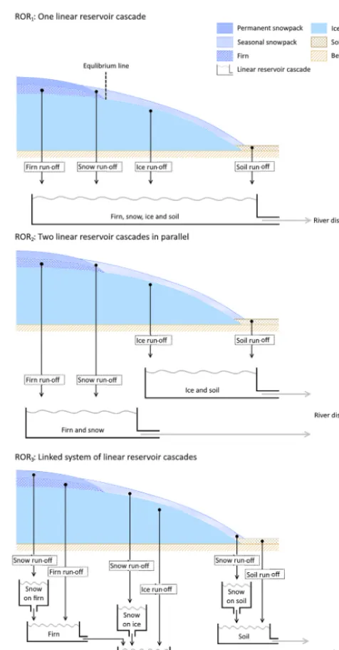
For temperate glaciers, common practice is to subdivide the catchment into one or more hydrological response units (HRUs) which are thought to have different water storage and release characteristics. For example, the firn, snow and bare ice have generally been shown to respond over rela-tively long, intermediate and short timescales respecrela-tively (Hock and Jansson, 2005), and therefore these may be char-acterised as separate HRUs, although as noted previously, simpler and more complex definitions of HRUs have been de-fined in the past. Subsequently, three run-off-routing model structures were proposed with different levels of complexity structured around these subdivisions (Fig. 2).
The first and simplest run-off-routing model structure (ROR1) uses a single linear reservoir cascade (e.g. Boscarello et al., 2014) to route the inflow from all run-off sources si-multaneously. This structure makes no distinction between the different run-off sources and flow pathways and assumes that all conform to the same storage–discharge relationship.
The second model structure (ROR2), employs two lin-ear reservoir cascades in parallel (e.g. Hannah and Gurnell, 2001). The first cascade represents the slow percolation of water through the snow and firn HRUs, while the second cas-cade represents a faster flow of water through the bare ice and overland. This approach therefore makes some distinc-tion between the different flow pathways and, by condidistinc-tion- condition-ing the parameters so that the snow and firn have a more dif-fuse response function, it introduces a degree of non-linearity in the discharge response to run-off.
The third run-off-routing model structure (ROR3) has not been used previously. It employs separate linear reservoir cascades to route water from the firn, snow, ice and soil
Figure 2.Three run-off-routing model structures which relate the linear reservoir cascade configurations to idealised cross sections of a temperate glacier.
out-Figure 3.Continuous hourly time series of precipitation(a), temperature(b)and incident solar radiation(c)between 1988 and 2015 at AWS1.
let (see Fig. 2c) and this represents the most complex, non-linear run-off-routing model structure.
2.4 Driving climate data
The GHM was configured to run from the initial ice geom-etry of 1988 to 2015. It requires continuous measurements of hourly precipitation, near-surface air temperature and in-cident solar radiation to drive the various model components. 2.4.1 Precipitation
A new gridded precipitation time series was constructed for the GHM, which incorporates the measurements of rainfall from the weather stations in the Virkisá basin and the infor-mation on spatial and long-term variations in precipitation from the gridded ICRA reanalysis product. First, the weather station rainfall data were used to correct the ICRA reanal-ysis product for bias. Given that none of the weather sta-tions are equipped with devices to measure snowfall, and that freezing temperatures can induce erroneous measurements in rainfall, only data with three consecutive preceding above-freezing days were used. This is a major issue when using AWS4, as the majority of days, particularly in the winter,
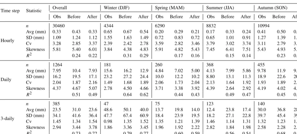
Table 1.Statistics calculated from the observed (Obs) precipitation data at AWS1 and from the corresponding ICRA precipitation data before and after bias correction. Statistics have been calculated at an hourly, daily and 3-daily time step and includen(total number of above-freezing measurements available at AWS1), avg (mean), SD (standard deviation), Cv (coefficient of variation), skewness and R2 (coefficient of determination).
Time step Statistic Overall Winter (DJF) Spring (MAM) Summer (JJA) Autumn (SON)
Obs Before After Obs Before After Obs Before After Obs Before After Obs Before After
Hourly
n 30460 4344 6290 8832 10994
Avg (mm) 0.33 0.43 0.33 0.65 0.67 0.54 0.20 0.29 0.21 0.17 0.33 0.24 0.41 0.50 0.39 SD (mm) 1.09 1.24 1.12 1.55 1.63 1.49 0.72 0.83 0.72 0.65 1.01 0.91 1.27 1.39 1.25
Cv 3.28 2.85 3.37 2.39 2.42 2.78 3.59 2.82 3.46 3.79 3.02 3.74 3.11 2.79 3.23
Skewness 5.81 5.40 6.01 3.84 4.38 4.83 5.91 4.82 5.43 7.45 6.41 7.51 5.43 4.93 5.35
R2 0.24 0.22 0.31 0.29 0.17 0.16 0.15 0.14 0.23 0.22
Daily
n 1264 181 260 368 455
Avg (mm) 7.95 10.4 7.93 15.6 16.2 12.9 4.84 7.02 5.00 4.13 7.99 5.86 9.78 11.9 9.31 SD (mm) 16.2 19.5 17.1 23.2 27.2 24.4 10.0 12.2 10.2 8.80 13.1 11.3 18.9 22.6 20.0
Cv 2.04 1.87 2.16 1.49 1.68 1.89 2.06 1.73 2.04 2.13 1.64 1.92 1.93 1.89 2.15
Skewness 4.37 4.67 5.07 2.78 4.50 4.66 3.71 3.38 3.92 4.39 2.64 2.92 4.19 4.02 4.36
R2 0.51 0.49 0.64 0.62 0.44 0.43 0.49 0.47 0.45 0.43
3-daily
n 385 47 75 123 140
Avg (mm) 23.5 31.0 23.6 48.6 50.1 40.0 13.7 19.8 14.0 12.4 23.8 17.4 30.0 36.8 28.7 SD (mm) 34.1 41.6 36.4 47.7 67.4 60.9 18.4 23.9 19.5 18.2 27.1 22.8 39.7 45.4 39.7
Cv 1.45 1.34 1.54 0.98 1.35 1.52 1.35 1.21 1.39 1.46 1.14 1.31 1.32 1.23 1.38
Skewness 2.94 3.44 3.78 1.86 3.36 3.45 1.96 1.92 2.22 2.82 1.84 1.98 2.58 2.28 2.53
R2 0.73 0.72 0.79 0.77 0.60 0.59 0.56 0.54 0.68 0.66
corrects for bias in the mean (Avg) and also improves the spread (SD), relative variability (CV) and skewness of the distribution of precipitation data at hourly, daily and 3-daily time steps. On a seasonal scale, these improvements are no-table for spring, summer and autumn. However, the bias-correction procedure typically has a slightly negative impact on the winter precipitation statistics, probably because of the limited above-freezing data available for these months. In particular, average hourly winter precipitation is underesti-mated by 0.11 mm (16 %), while the positive bias in relative variability and skewness are amplified after bias correction. Given that EQM preserves the rank correlation of the time series, it has little effect on the R2 correlation score, with a typical reduction of 0.01–0.02 after bias correction. At an hourly timescale, the bias-corrected data only captured 22 % of the observed variance in the AWS1 rainfall record. How-ever, when averaged to a daily time step the R2 score in-creased to 0.49, and for a 3-daily time step theR2increased to 0.72. The limited correlation of the ICRA precipitation data on an hourly timescale could hinder the acceptability of the GHM across some of the signatures (e.g. the river dis-charge signatures related to the timing of flows). However, the AWS1 rainfall record is complete for the years 2013 and 2014 for which the GHM is compared against observed river discharge signatures. As such, poor replication of the timing of hourly rainfall events should have minimal influence on the GHM’s ability to capture the river discharge signatures. Rather, the role of the bias-corrected ICRA precipitation data was primarily to drive the glacier mass balance component of
the GHM prior to 2009 for which a reliable 3-daily temporal correlation with observations was deemed adequate. 2.4.2 Near-surface air temperature
The longest record of hourly temperature measurements in the Virkisá River basin are from AWS1, which starts in 2009. To generate a continuous time series of temperature back to 1988, daily measurements of temperature available from the nearby Fagurhólsmýri weather station were used. A com-parison of daily average temperatures showed there to be a good linear relationship between the two stations with anR2 of 0.92. As such, this linear model was used to correct the daily weather station data for bias so that it could be com-bined with the AWS1 time series. To downscale the data to an hourly resolution, 24 h temperature anomalies were ran-domly sampled from the AWS1 record, thereby ensuring the complete time series had a consistent subdaily variability. Of course, diurnal cycles in temperature are dependent on the time of year, in that increased incident solar radiation in the summer enhances subdaily temperature variability. There-fore, the sampling strategy was employed on a month-by-month basis. The complete hourly time series of temperature at AWS1 is shown in Fig. 3b.
In fact, while many studies employ a fixed temperature lapse rate, in reality seasonal variations in surface characteristics (e.g. albedo and roughness) and atmospheric conditions can bring about strong seasonal and diurnal variations in lapse rates which control melt processes (Gardner et al., 2009; Minder et al., 2010; Immerzeel et al., 2014). Furthermore, local atmospheric phenomena associated with midlatitude glaciers, such as katabatic winds which bring cool dense air over the ice surface, can serve to reduce the tempera-ture gradient (Petersen and Pellicciotti, 2011; Ragettli et al., 2014). Having analysed near-surface air temperature varia-tions both on and away from the Virkisjökull glacier, it was deemed most appropriate to extrapolate temperature across the study catchment using a seasonally variable hourly lapse rate in conjunction with an on-ice temperature correction function based on the work of Shea and Moore (2010) (see Appendix B).
2.4.3 Incident solar radiation
The only source of incident solar radiation is the ous hourly time series from AWS1. To construct a continu-ous time series back to 1988, a resampling strategy was em-ployed to generate a complete time series that was statisti-cally consistent with the data at AWS1. It was found that, during the summer months, the daily range in incident so-lar radiation and temperature are strongly correlated. There-fore, when generating a continuous time series of hourly inci-dent solar radiation from 1988, it was important to maintain this dependence between intra-day solar radiation and tem-perature variability. To do this, a coordinated (in time) sam-pling strategy identical to that used for the near-surface air temperature data was employed. More specifically, for each random 24 h temperature anomaly sample from the AWS1 record used to build part of the temperature time series, the corresponding 24 h solar cycle data were extracted and used to build the same part of the incident solar radiation time se-ries. Figure 3c shows the complete time series of incident solar radiation used to drive the model.
2.5 Signatures and limits of acceptability
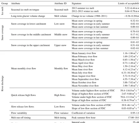
Observations of ice melt, snow coverage and river discharge were used to derive 33 unique signatures with LOA to char-acterise the glacio-hydrological behaviour of the Virkisá River basin over different spatio-temporal scales and eval-uate the acceptability of the different model structures (Ta-ble 2). For convenience, the signatures have also been subdi-vided into 11 attributes which encapsulate the main aspects of model behaviour that were assessed.
2.5.1 Ice melt
The average winter (November 2012–April 2013) and sum-mer (May 2013–September 2013) melt across the ablation stake network were used to characterise the short-term,
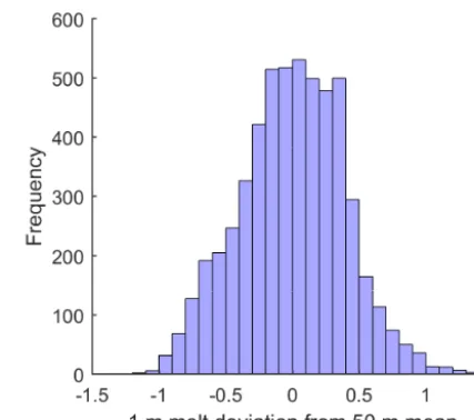
sea-Figure 4.Histogram of deviation of 1 m melt from 50 m mean de-rived from terrestrial lidar scans of static ice front between 2012 and 2014.
sonal ice melt on the glacier tongue. Of course, point mea-surements of melt are not directly comparable to simulated melt at the GHM nodes as these simulations represent the average melt over the node area. Therefore, the GHM can only be expected to get as close to the stake measurements as the actual spread in melt over the equivalent model node area. To calculate this spread, the high-resolution terrestrial lidar scans taken during the ablation stake campaign were used. The scans were used to estimate the spread of melt deviations from the mean melt across 50 m square regions (Fig. 4). The 95 % confidence bounds (±0.78 m yr−1) were then used to define the LOA around the winter and summer melt signatures where it was assumed that the spread should be proportional to the total melt. This assumption leads to much narrower LOA around the winter melt signature than the summer melt signature.
Table 2.Summary of signatures used to evaluate model acceptability. Units with an asterisk (*) are per section of flow duration curve.
Group Attribute Attribute ID Signature Limits of acceptability
Ice
melt Seasonal ice melt on tongue Seasonal melt
2013 summer ice melt 5.22–6.44 m we
2012–2013 winter ice melt 0.64–0.78 m we
Long-term glacier volume change Melt volume Change in ice volume (1988–2011) −0.36–0.28 km3
Sno
w
co
v
erage
Snow coverage in lower catchment Low snow
Mean snow coverage in spring 0.32–0.45
Mean snow coverage in early summer 0.02–0.08
Mean snow coverage in late summer 0.00–0.03
Snow coverage in the middle catchment Middle snow
Mean snow coverage in spring 0.70–0.80
Mean snow coverage in early summer 0.17–0.27
Mean snow coverage in late summer 0.00–0.04
Snow coverage in the upper catchment Upper snow
Mean snow coverage in spring 0.81–0.90
Mean snow coverage in early summer 0.51–0.64
Mean snow coverage in late summer 0.02–0.09
Ri
v
er
dischar
ge
Mean monthly river flow Monthly flow
Mean January river flow 1.16–1.86 m3s−1
Mean February river flow 1.69–2.92 m3s−1
Mean March river flow 0.85–1.58 m3s−1
Mean April river flow 0.73–1.48 m3s−1
Mean May river flow 1.50–2.16 m3s−1
Mean June river flow 4.12–6.23 m3s−1
Mean July river flow 6.33–10.30 m3s−1
Mean August river flow 5.72–9.15 m3s−1
Mean September river flow 4.55–7.38 m3s−1
Mean October river flow 3.88–7.02 m3s−1
Mean November river flow 3.90–7.40 m3s−1
Quick release high flows High flows
Volume under highest-flow section of FDC 59.4–116.0 m3s−1* Slope of highest-flow section of FDC 2.67–9.88 m3s−1* Volume under high-flow section of FDC 70.6–111.0 m3s−1* Slope of high-flow section of FDC 0.38–0.79 m3s−1*
Slow release low flows Low flows Volume under low-flow section of FDC 20.9–46.1 m
3s−1* Slope of low-flow section of FDC 0.03–0.05 m3s−1*
Flow variability Flow variance Coefficient of variation 0.95–1.83
Melt run-off timing Melt timing Peak summer flow hour 17:00–18:00
Flashiness Flow flash Integral scale 25–44 h
Rising limb density 0.13–0.20
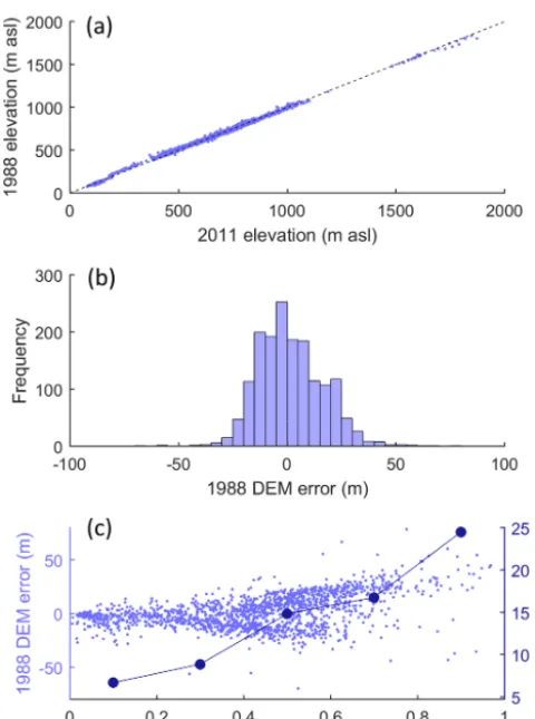
drawn from a normal distribution with mean zero. Given that the spread of the residuals increases for those areas of the catchment that are steepest, the shape parameter of the er-ror distribution (standard deviation) was varied according to the slope of each pixel of the 1988 DEM (see dark-blue line in Fig. 5c). From these, 1000 equally probable estimates of ice volume change were calculated and the 95 % confidence interval was used to define the LOA. The total change in ice volume over 23 years from 1988 was estimated to be between
−0.36 and−0.28 km3. 2.5.2 Snow coverage
Having removed the MODIS data that did not pass the QA test including all of the data between September and
Figure 5. Error model for estimating uncertainty in glacier vol-ume change between 1988 and 2011 including 1988 vs. 2011 off-ice DEM elevations (a), distribution of 1988 DEM errors calcu-lated as the difference between 1988 and 2011 off-ice elevations
(b) and estimation of change in standard deviation of errors with the DEM slope(c).
that covered ice-free parts of the catchment were used. This limited the analysis up to a maximum elevation of just un-der 1200 m a.s.l. While this does not cover the full elevation range of the catchment, Fig. 6 shows that the three curves capture a large amount of variability in seasonal snow cover. From the three snow coverage curves, the mean snow cover-age values from the lower, middle and upper terciles of the curves were used as signatures of snow coverage.
There exists no definitive quantification of errors in the MOD10A1 product that can be used to estimate LOA for these signatures. Previous validation of the MODIS data us-ing satellite imagery has shown the data to be relatively ro-bust (Salomonson and Appel, 2004). Accordingly, it was assumed that, as with the ablation stake data, the primary source of uncertainty stems from scale differences between the data and the model simulations. More specifically, be-cause the MODIS data have a coarser resolution (500 m) than the DEM over which the MODIS data were distributed (50 m), a MODIS pixel value of 0.5 only indicates that 50
of the corresponding 100 DEM pixels are snow covered. The construction of a snow distribution curve, therefore neces-sitates some assumptions about where the snow actually lies which will influence the shape of the snow distribution curve. Accordingly, the LOA were quantified to account for this uncertainty. Here, for each of the seasons, a mean MODIS snow cover map over the study region was derived. Then, for each 500 m pixel, snow was randomly distributed across the corresponding DEM pixels 1000 times. From these, an equal number of snow distribution curves and corresponding snow distribution signatures could be derived, each of which were assumed to be equally probable. The 95 % confidence bounds from this distribution of snow cover signatures were used to define the LOA which are indicated by blue error bars in Fig. 6.
2.5.3 River discharge
The hourly river discharge data for the years 2013 and 2014 measured at ASG1 (Fig. 7a) were used to define 21 differ-ent river discharge signatures that cover a range of temporal scales and flow magnitudes. The majority of these signatures were based on previous studies (e.g. Yadav et al., 2007; Yil-maz et al., 2008; Shafii and Tolson, 2015; Schaefli, 2016).
Mean monthly river flows were calculated to characterise the seasonal river flow regime. Signatures were also de-rived from sections of the flow duration curve to characterise quick-release high flows and slow-release low flows. These include signatures that quantify the volume under the section (flow magnitude) and the slope of section (flow variability) for the low-flow section (99–66 % flow exceedance), high-flow section (15–5 % high-flow exceedance) and highest-high-flow sec-tion (5–0.5 % flow exceedance). An overall estimate of flow variability, the coefficient of variation, was also calculated. Related to this, two further signatures, the rising limb den-sity and integral scale, provide a measure of flashiness. The rising limb density is the ratio of the number of flow peaks to the total time to peak where a higher number is more flashy. The integral scale measures the lag time at which the au-tocorrelation function of the flow time series falls below 1e (diurnal cycles in river flow were removed prior to this using a moving average filter). A higher integral scale therefore in-dicates a less flashy, slowly responding hydrological system. Finally, the peak summer flow hour of the observed discharge time series was calculated to characterise the intra-day river discharge response to melt.
un-Figure 6.Snow coverage curves defined from the MOD10A1 snow cover product from 2000 to 2015 with 95 % confidence bounds.
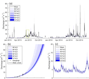
Figure 7.River flow time series from ASG1 with quantified confidence intervals(a), rating curve uncertainty used to quantify confidence intervals(b)and zoomed section of river flow time series (see yellow dashed box in top plot) with confidence intervals(c).
certainty stems from the assumptions hydrologists have to make when constructing rating curves, such as assuming the river bed profile and horizontal flow velocity distribution are relatively stable over time. These errors make fitting a single rating curve to all of the gauging data invalid. Accordingly, McMillan and Westerberg (2015) propose a method to define the rating curve uncertainty which accounts for both sources of error and has been used to estimate uncertainty in river discharge signatures (Westerberg et al., 2016). The random error component was defined from analysis of 27 flow gaug-ing stations in the UK with stable ratgaug-ings and without obvious
epistemic errors (Coxon et al., 2015). They conclude that this source of error is best approximated by a logistical distribu-tion model. To account for the epistemic error, they reject the assumption that the rating curve is fixed in time and instead they fit an ensemble of rating curves to all of the gauging data. Each curve is weighted by a “voting point” likelihood function which scores it based on how many points of the pe-riodic gaugings it is able to intersect (and at what location in the logistical distribution of each measurement).
uncer-tainty. Markov chain Monte Carlo sampling was used to de-fine 667 unique rating curves which together dede-fine the rat-ing curve uncertainty (Fig. 7b). From these an equivalent dis-tribution of each river discharge signature was derived from the ensemble of flow time series (Fig. 7c), from which the 95 % confidence bounds were used as the LOA. Because the voting point method only accounts for uncertainty in the flow magnitude and not the timing, it was not suitable to apply this approach to the three signatures that charac-terise melt run-off timing and flashiness. For these signa-tures, Schaefli (2016) proposed that the LOA should be de-rived by subsampling different periods of the flow time se-ries. For this study a month-by-month subsampling strategy was employed to do this.
2.6 Model calibration procedure
The GHM was configured to run from 1988 to 2015 so that simulations could be compared against all observation sig-natures. The initial ice surface was set to the 1988 DEM of the ice, while the bedrock and land surface topography were taken from the Öræfajökull bedrock map (Magnússon et al., 2012). Initial snow coverage, soil moisture, linear reservoir storages and ELA were determined by running the model for 3 consecutive years prior to the simulation period using cli-mate data from 1985 to 1988.
In total there were nine possible structural configurations of the GHM including all possible combinations of the three melt and run-off-routing model structures. For each of the nine configurations, the melt and run-off-routing model pa-rameters were calibrated to achieve the closest fit to the ob-served signatures. To do this, first a set of preliminary runs were undertaken to assess the sensitivity of the simulations to the parameters. Here, it was found that the simulations were insensitive to the firn melt parameters across the range of 33 signatures. Accordingly, these were set to the same values as for snow. Similarly, none of the signatures were sensitive to the threshold above which melt occurs,T∗, and accordingly, this was set to 0◦C throughout the model experiments. Fi-nally, it was also decided to fix the albedo parameter for ice in TIM3to 0.3. This was because this parameter directly in-teracts with thebparameter and therefore provides no extra control over model behaviour.
The remainder of the parameters were kept for calibration (see Table C1). For each GHM configuration, 5000 Monte Carlo simulations with random parameter sets sampled from predefined uniform distributions were undertaken. The prior parameter distributions were defined from a review of pre-vious modelling studies and later refined during the prelim-inary runs noted above. The quasi-random Sobol sampling strategy (Brately and Fox, 1988) was employed to sample the parameter space as efficiently as possible. The simulated signatures from each model run (parameter set) were then evaluated against the observed signatures using a continuous
acceptability score:
sj =
0 lowj≤simj≤uppj simj−uppj
uppj−obsj simj>uppj
simj−lowj
obsj−lowj simj<lowj
, (9)
where obsj and simj are the observed and simulated values for signaturej and uppj and lowj are the upper and lower LOA. Here, a score of zero indicates that the model captures the observed signature within the LOA. An absolute score greater than 0 is outside of the LOA and therefore unaccept-able. The sign of the score indicates the direction of bias, while its magnitude indicates the model’s performance rela-tive to the LOA. A score of−3 would indicate that the model underestimates the signature by 3 times the observation un-certainty.
Given that there are 33 different signatures to calibrate to simultaneously, it was important to define a weighting scheme to achieve the best overall performance across the range of signatures. It was decided that, for a given GHM configuration, the 5000 runs should be ranked by a weighted average score where each group, each attribute within each group and each signature within each attribute were given equal weighting so that the scores were not biased to a par-ticular group or attribute. The top 1 % of model runs that achieved the smallest weighted average acceptability scores were then taken as the calibrated models for each GHM configuration and the average acceptability scores of these are reported. A bootstrapping with a replacement resampling scheme was also used to assign 95 % confidence intervals around all reported acceptability scores. While not a formal test of statistical significance, these were used to avoid re-porting differences between the GHM configurations where issues such as undersampling of the parameter space would make such conclusions unjustified. Where confidence in-tervals do not overlap, differences are hereafter referred to as substantial. The different GHM configurations were also compared when calibrated to individual groups of signatures (ice melt, snow coverage and river discharge). In this case the same weighting procedure was applied to a single group only.
3 Results
3.1 Signature discrimination power
constrain the range of acceptable model compositions. Here, the total number of acceptable model compositions were cal-culated for each signature as an indicator of discrimination power (bars in Fig. 8a). The results indicate that the ice melt signatures are the best discriminators. Of these, the winter melt signature from the ablation stake measurements is the best discriminator, while the summer melt signature shows the least discrimination power. The snow coverage signatures generally are shown to be inferior discriminators when com-pared to the ice melt signatures. The late-summer snow cov-erage signature for the lower catchment is shown to be the poorest discriminator, presumably because there is negligible snow cover here at this time of the year: an observation that almost all of the model compositions have no difficulty in replicating. In contrast, no model compositions are deemed acceptable for the signatures of the spring and early-summer snow coverage in the upper catchment.
The discrimination power of the river discharge signatures is shown to be highly variable, but there are several dis-cernible patterns. Firstly, the mean monthly flow signatures between January and June, when river discharge is low, are shown to be better discriminators than the higher-flow sig-natures from July to October. The mean monthly January and May flows stand out as being particularly powerful at discriminating between acceptable and unacceptable model compositions, suggesting that these are likely to be focal points for characterising model deficiencies. Those signa-tures related to the variability of flows such as the coefficient of variation and the flow duration curve slope signatures, as well as peak flow hour (timing) and rising limb density (flashiness) are also shown to be relatively good discrimina-tors.
To determine the structural discrimination power of each signature, the total number of GHM configurations that re-turned at least one acceptable simulation have also been cal-culated for each signature (scatter in Fig. 8a). They show that, when used individually, most of the discrimination power stems from constraining the parameter space rather than constraining the structural space. Only the lower-catchment spring snow coverage and mean January river flow signa-tures discriminate between strucsigna-tures where only six of the nine GHM configurations returned acceptable simulations. In both cases it was the GHM configurations that employed the TIM3melt model structure that could not capture these signatures within their LOA.
To indicate how each signature helps to reduce river flow prediction uncertainty, a second measure of discrimination power has also been calculated (Fig. 8b). Here, the mean simulated range in river discharge from the population of ac-ceptable models has been calculated as a percentage of the simulated range using all of the 45 000 model compositions for each signature. These results show that when used indi-vidually, all of the signatures help to constrain the river flow prediction uncertainty, although the effectiveness of each is variable. The mean January and May river flow signatures
again exhibit good discrimination power, reducing the mean river discharge uncertainty to 60–70 % of that from the full population of model compositions. Similarly, the winter ice melt and spring snow coverage in the lower catchment re-main two of the best discriminators. However, some signa-tures, such as the long-term volumetric change in the glacier, which was a good discriminator of model acceptability, are not as effective at reducing river discharge prediction uncer-tainty.
3.2 Acceptability of melt model structures
While all signatures clearly demonstrate discrimination power when used individually, it remains to be seen how ef-fective the LOA framework is for discriminating between and diagnosing deficiencies in different model structures when using multiple evaluation criteria. Here, the acceptability scores obtained after calibrating the GHM to the different groups of signatures (ice melt, snow coverage and river dis-charge) using the three different melt model structures have been calculated (Fig. 9). The light-grey boxes indicate those signatures that have been captured within the LOA, and the dark-grey boxes and their corresponding acceptability scores indicate those signatures which the structures were not able to capture within the LOA. So that the river discharge ac-ceptability scores can be compared fairly, they have all been obtained using the ROR1run-off-routing structure.
When calibrated against the ice melt signatures, the GHM is not able to capture them within their LOA, regardless of the melt model structure used. The different GHM configu-rations show a tendency to overestimate the measured sum-mer and winter melt from the ablation stake data, yet un-derestimate the long-term change in total ice volume (note underestimation here refers to the simulated loss in ice vol-ume). This highlights a deficiency in the melt model struc-tures as they are unable to reconcile the three melt signastruc-tures simultaneously within the observation uncertainty. The win-ter melt is by far the most unacceptable simulation, particu-larly when using the TIM1structure, which overestimates it by more than 30 times the observation uncertainty.
Each of the GHM configurations using the three melt model structures have been ranked from 1 to 3 in the top left corner of each box where the acceptability scores are substantially different (Fig. 9). While there are clearly dif-ferences in the acceptability scores for the summer melt and ice volume signatures, they are not substantially differ-ent and therefore it is not possible to say that one structure is more acceptable than another. Indeed, a comparison of the simulated ice thickness change along the Falljökull and Virkisjökull arms of the glacier reveal that all three config-urations of the GHM produce almost identical simulations which broadly capture the observed ice thickness change be-tween 1988 and 2011 (Fig. 10).
struc-Figure 8.Total number of acceptable model compositions (bars) and configurations (dots) for each signature(a)and mean simulated range in river discharge from the population of acceptable models as a percentage of the simulated range using all of the 45 000 model composi-tions(b).
tures. Here, the GHM configuration using the TIM3structure is the most acceptable, while using the TIM1structure is least acceptable, indicating that, while all configurations produce simulations outside of the LOA, there is an improvement in ice melt simulations when implementing the most sophisti-cated TIM3melt model structure.
For the snow coverage signatures, all three of the GHM configurations capture the late-summer snow coverage in the lower portion of the catchment within the LOA. When us-ing the TIM2and TIM3structures, the mid-catchment spring snow coverage is also captured. The remaining snow cov-erage signatures are not captured within the LOA, where all configurations show a tendency to underestimate snow cage in the lower and middle parts of the catchment and over-estimate snow coverage in the upper part of the catchment. To investigate why this is, Fig. 11a shows the simulated
early-summer mid-catchment and upper-catchment snow coverage signatures for the 5000 calibration parameter sets (blue dots) used with the TIM1–ROR1GHM configuration. Here it can be seen that, regardless of the choice of melt model parame-ters, this structure is not able to capture both of these signa-tures within their LOA simultaneously (indicated by yellow area). A similar inconsistency exists when comparing snow coverage over different seasons where the GHM is not able to capture the lower-catchment snow coverage in the early summer and spring simultaneously (Fig. 11b). Indeed, this inconsistency extends across all melt model structures.
Figure 9.Acceptability scores obtained after calibrating the GHM using the three melt model structures in combination with the ROR1 run-off-routing model structure. The three GHM configurations were calibrated against ice melt, snow coverage and river discharge signa-tures separately. Light-grey boxes indicate acceptable simulations (s=0) and numbered, dark-grey boxes indicate unacceptable simulations coloured blue and red to indicate negative and positive biases respectively. Note that all acceptability scores are rounded to two decimal places. Those non-zero scores that round to zero are accompanied by±to indicate sign of score. White numbers in the top left of each box indicate relative ranking where acceptability scores are substantially different between the GHM configurations.
structure has a limited influence on the simulated seasonal snow coverage.
The acceptability scores for the river discharge signatures in Fig. 9 show that, regardless of the choice of melt model structure, when used in conjunction with the ROR1 run-off-routing model structure, all are able to capture a range of river discharge signatures. The simplest GHM configura-tions using the TIM1and TIM2model structures capture 12 river discharge signatures simultaneously within the LOA, while the inclusion of the dynamic snow albedo term and re-arrangement of the melt equation in the TIM3 melt model
actually inhibits the GHM performance where only 10 of the 21 river discharge signatures are captured within the LOA.
Figure 10.Observed and simulated ice thickness change as measured along the transects of the Falljökull and Virkisjökull glacier arms. Insets show transect locations.
Figure 11.Simulated snow coverage signatures from the 5000 calibration runs (blue dots) for the TIM1-ROR1GHM configuration includ-ing early-summer mid-catchment and upper-catchment snow coverage signatures(a), and lower-catchment spring and early-summer snow coverage signatures(b).
three melt model structures (Fig. 13a), which results in a pos-itively biased river flow time series (see Fig. 13b). Note that the full input/output time series over the observation period can be found in Appendix D.
Furthermore, a comparison of the simulated ice melt time series over 2013 with a monthly moving-average filter demonstrates that the positive melt bias from TIM3extends between April and June (Fig. 14b), which corresponds to the period in which temperatures are relatively low but incoming solar radiation is relatively high (see Fig. 14a).
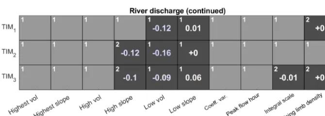
Of the remaining river discharge signatures, only a handful show any substantial difference when switching between the melt model structures including the mean April and August discharge and the two flashiness signatures: the integral scale and the rising limb density. However, the differences here are very small. For the high-slope signature, which characterises
the variability of high-flow river flows, the simulation using the TIM1 melt model structure is able to capture it within the LOA, while the simulations using the TIM2 and TIM3 model structures both show a negative bias, suggesting they underestimate high-flow variability.
3.3 Acceptability of run-off-routing model structures To evaluate the run-off-routing model structures, acceptabil-ity scores have been calculated for the river discharge signa-tures only, as these strucsigna-tures do not influence ice melt or snow coverage (Fig. 15). To ensure a fair comparison be-tween the different structures, all scores have been obtained using the simplest TIM1melt model structure in the GHM.
Figure 12.Simulated seasonal snow distribution curves when using the three melt model structure.
Figure 13. Mean simulated hourly ice melt (a) and river dis-charge(b)during May 2013 using the top 1 % of models from the three melt model structures in combination with the ROR1 run-off-routing model structure.
more complex non-linear run-off-routing model structure in the GHM could help to mitigate this bias. Indeed, the cali-brated simulations do show a substantial reduction in posi-tive bias for the mean February flows when using ROR2and ROR3; however the simulations are still unacceptable. Fur-thermore, for the mean January river flow there is no sub-stantial change in acceptability score.
This indicates that the run-off-routing representation is also not the reason for the overestimation of flows at the be-ginning of the year. To investigate this positive bias further, Fig. 16c shows the simulated time series from the calibrated models using TIM1in combination with ROR1, ROR2and ROR3for January and February 2013. Figure 16a shows that input from melt is insignificant during these winter months
Figure 14. Normalised temperature and incident solar radiation
(a)and simulated ice melt from the three calibrated ice melt model structures(b)for the year 2013. All time series use a monthly mov-ing average filter.
deficien-Figure 15.Acceptability scores obtained after calibrating the GHM using the three run-off-routing model structures in combination with the TIM1melt model structure. Light-grey boxes indicate acceptable simulations (s=0) and numbered dark-grey boxes indicate unacceptable simulations, coloured blue and red to indicate negative and positive biases respectively. Note that all acceptability scores are rounded to two decimal places. Those non-zero scores that round to zero are accompanied by±to indicate sign of score. White numbers in top left of each box indicate relative ranking where acceptability scores are substantially different between the GHM configurations.
cies, however, all result in an almost identical positive bias as shown by the cumulative flow in Fig. 16b.
There are, however, differences when assessing other as-pects of the river discharge time series, particularly in the sig-natures relating to high flows. In Fig. 15, it can be seen that, while the simulation using the ROR1-routing model structure is able to capture all of the high-flow signatures simultane-ously, the ROR2and ROR3structures show an unacceptable negative bias for these signatures, indicating underestimation of high-flow magnitude and variability. To evaluate this in more detail, Fig. 16f shows the simulated time series for the highest recorded river flow event during October 2014. Here, the flashier and more responsive ROR1structure achieves the closest fit to the observed peak flow and within the uncer-tainty bounds, while the more diffusive, ROR2 and ROR3 structures underestimate the peak flow. Note they also under-estimate the overall river flow variability as indicated by the coefficient of variation signature.
3.4 Consistency of melt model structures
The results so far have highlighted some inconsistencies in the GHM configurations using the melt and run-off-routing model structures, which are unable to reconcile some
com-binations of signatures simultaneously. This is important as those inconsistencies could help to further diagnose struc-tural deficiencies in the different model structures. To inves-tigate this, consistency scores have been calculated between pairs of the 33 signatures for each GHM configuration. A model can be deemed consistent across a pair of signatures if it is able to capture them within their LOA simultaneously. The consistency scores are therefore calculated as the mini-mum sum of the two acceptability scores between a pair of signatures across the 5000 calibration runs for each GHM configuration.
demon-Figure 16.Simulation time series using the three different run-off-routing model structures in combination with the TIM1melt model structure including simulated total melt and rainfall (a), cumula-tive river discharge (middle) and river discharge time series (bot-tom) for January and February 2013(a, b, c)and the October 2014 flood(d, e, f).
strates that, when using the TIM1structure, the GHM cannot reconcile the upper-catchment snow coverage with any of the other attributes.
The largest inconsistency score obtained was between the short-term, seasonal melt on the glacier tongue and long-term total glacier volume change. It should be noted that the sea-sonal melt signatures show a small inconsistency with the lower-catchment snow coverage and a larger inconsistency with the upper-catchment snow coverage. The total glacier volume change signature, however, is also inconsistent with the monthly flow and low-flow signatures, indicating that it is the long-term glacier wide mass balance that the model is getting wrong.
The use of the TIM2 model structure, which includes topographic effects, goes some way to reducing most of the inconsistencies shown using the TIM1 model structure (Fig. 17). However, all but one of the inconsistencies (be-tween lower-catchment snow coverage and seasonal melt) remain, indicating that the use of the TIM2melt model struc-ture only provides a small improvement in model consis-tency.
Using the TIM3 model structure also helps to improve model consistency, particularly for the upper snow cover-age signatures, but surprisingly it also introduces new incon-sistencies in relation to the lower-catchment snow coverage, where the model is not able to reconcile these signatures with any of the other attributes.
3.5 Consistency of run-off-routing model structures
incon-Figure 17.Average consistency scores between attributes using the three melt model structures in combination with the ROR1 run-off-routing structure. Scores of<0.1 have not been reported.
sistencies, particularly when using the ROR3model structure where the inconsistencies extend into June (bottom panel).
The ROR1simulations show inconsistencies between the February flows and low-flow variability as indicated by the low-slope signature. The reason for this is not clear, but in-terestingly, the inclusion of an extra, more diffuse, flow path-way in the ROR2model appears to remedy this, suggesting that there is some non-linear behaviour that the ROR1model structure cannot capture. However, it comes at the cost of inducing an extra inconsistency between the mean flows in January and the overall flow variability as indicated by the coefficient of variation. This new inconsistency is amplified when using the ROR3structure.
Interestingly, the consistency scores when using the ROR1 and ROR2 structures are relatively similar, with each con-figuration demonstrating inconsistencies between four and five pairs of river discharge signatures. In contrast, using the most complex ROR3 structure introduces a number of new inconsistencies with a total of 12 inconsistent pairs of sim-ulated river discharge signatures. These new inconsistencies are centred around the mean monthly flow signatures as well as the signatures relating to high- and low-flow magnitude and variability.
4 Discussion
The first aim of this study was to investigate whether a signature-based approach within a LOA framework could be used to diagnose deficiencies in the different melt and run-off-routing model structures. The comprehensive set of sig-natures provided a powerful method with which to evaluate the model behaviour. Furthermore, when used within a LOA framework, it was straightforward to identify those aspects of the glacio-hydrological system that the GHM configurations could not capture. A number of the identified model deficien-cies are particularly important in the context of future river flow predictions, which will now be discussed.
re-Figure 18.Average consistency scores between river discharge sig-natures using the three run-off-routing model structures in combi-nation with the TIM1melt model structure.
quired to achieve acceptable model simulations that capture all of the ice melt signatures simultaneously. Certainly, one aspect of the glacier which was not accounted for was debris cover at the glacier terminus, which could be an important control for point scale and overall ice mass balance. Some TIMs that include representations of debris cover do exist (e.g. Carenzo et al., 2016) and the signature-based LOA ap-proach would provide the ideal framework for evaluating the added value of further structural modifications like these.