https://doi.org/10.5194/tc-13-1283-2019
© Author(s) 2019. This work is distributed under the Creative Commons Attribution 4.0 License.
Estimating the snow depth, the snow–ice interface temperature,
and the effective temperature of Arctic sea ice using
Advanced Microwave Scanning Radiometer 2 and
ice mass balance buoy data
Lise Kilic1, Rasmus Tage Tonboe2, Catherine Prigent1, and Georg Heygster3
1Sorbonne Université, Observatoire de Paris, Université PSL, CNRS, LERMA, Paris, France 2Danish Meteorological Institute, Copenhagen, Denmark
3Institute of Environmental Physics, University of Bremen, Bremen, Germany
Correspondence:Lise Kilic ([email protected])
Received: 17 October 2018 – Discussion started: 12 November 2018 Revised: 1 April 2019 – Accepted: 2 April 2019 – Published: 18 April 2019
Abstract. Mapping sea ice concentration (SIC) and under-standing sea ice properties and variability is important, es-pecially today with the recent Arctic sea ice decline. More-over, accurate estimation of the sea ice effective temperature (Teff) at 50 GHz is needed for atmospheric sounding
applica-tions over sea ice and for noise reduction in SIC estimates. At low microwave frequencies, the sensitivity to the atmo-sphere is low, and it is possible to derive sea ice parame-ters due to the penetration of microwaves in the snow and ice layers. In this study, we propose simple algorithms to derive the snow depth, the snow–ice interface temperature (TSnow−Ice) and theTeff of Arctic sea ice from microwave
brightness temperatures (TBs). This is achieved using the Round Robin Data Package of the ESA sea ice CCI project, which contains TBs from the Advanced Microwave Scan-ning Radiometer 2 (AMSR2) collocated with measurements from ice mass balance buoys (IMBs) and the NASA Opera-tion Ice Bridge (OIB) airborne campaigns over the Arctic sea ice. The snow depth over sea ice is estimated with an error of 5.1 cm, using a multilinear regression with the TBs at 6, 18, and 36 V. TheTSnow−Iceis retrieved using a linear
regres-sion as a function of the snow depth and the TBs at 10 or 6 V. The root mean square errors (RMSEs) obtained are 2.87 and 2.90 K respectively, with 10 and 6 V TBs. The Teff at
microwave frequencies between 6 and 89 GHz is expressed as a function ofTSnow−Iceusing data from a
thermodynam-ical model combined with the Microwave Emission Model
of Layered Snowpacks.Teff is estimated from theTSnow−Ice
with a RMSE of less than 1 K.
1 Introduction
In situ observations of the variables controlling the sea ice energy and momentum balance in polar regions are scarce. One way to overcome this observational gap is to use satel-lites for measuring sea ice properties. The objective of this study is to estimate key sea ice variables from satellite remote sensing to improve current sea ice models and prediction, sea ice concentration (SIC) mapping in the EUMETSAT Ocean and Sea Ice Satellite Application Facility (OSISAF) project, and polar atmospheric sounding applications.
sea ice growth has been effectively limited by the increase in snow depth on thin ice during winter. Current sea ice models include snow schemes (e.g. Lecomte et al., 2011), with the snow depth and temperature gradient in the snow pack mod-ulating the sea ice growth and melt. Improved estimates of snow depth (Ds), as well as snow–ice interface temperature
(TSnow−Ice) from satellite observations would provide
valu-able information on the vertical thermodynamics in the snow and ice to improve current sea ice models and therefore the prediction of sea ice growth.
Here we propose using a simple algorithm to retrieveDs
and TSnow−Ice from passive microwave observations from
the Advanced Microwave Scanning Radiometer 2 (AMSR2), based on a large data set of collocated in situ and satel-lite observations. An extensive Round Robin Data Package (RRDP) (Pedersen et al., 2018, https://figshare.com/articles/ Reference_dataset_for_sea_ice_concentration/6626549, last access: 15 January 2019) has been developed during the Eu-ropean Space Agency (ESA) sea ice Climate Change Initia-tive (CCI) project and the SPICES (Space-borne observa-tions for detecting and forecasting sea ice cover extremes) project (http://www.seaice.dk/ecv2/rrdb-v1.1/, last access: 15 June 2017). It contains in situ data from the ice mass balance buoys (IMBs), and the Operation Ice Bridge (OIB) airborne campaigns collocated with AMSR2 brightness tem-perature measurements between 6 and 89 GHz.
Algorithms already exist to retrieve the snow depth from microwave observations. Markus and Cavalieri (1998) and Comiso et al. (2003) use the spectral gradient ratio of the 19 and 37 GHz (GR37/19) in vertical polarization to deduce the snow depth over sea ice. This method has been developed for dry snow on first-year ice (FYI) in Antarctica, and it is applicable only to this ice type. Sea ice emissivity depends on the ice type. At frequencies≥18 GHz, the ice emissivity is higher for FYI than for multi-year ice (MYI) (Comiso, 1983; Spreen et al., 2008). The difference of emissivity between the 19 and 37 GHz can be used to retrieve the snow depth or the sea ice type. Therefore, the snow depth algorithms which use this gradient ratio (GR37/19) are strongly dependent on the ice type. Improvements by Markus and Cavalieri (1998) have been suggested by Markus et al. (2011) and Kern and Ozsoy-Çiçek (2016). More recently, Rostosky et al. (2018) revisit the methodology for the Arctic region, using a new gradient ratio between 7 and 19 GHz (GR19/7) to derive snow depths over both FYI and MYI. For their study, they use the snow depths of OIB campaigns obtained in March and April. With the help of the RRDP, we will extend the methodology to the full winter (from 1 December to 1 April) for the Arctic region using the IMB snow depth data.
Tonboe et al. (2011) showed from radiative transfer sim-ulations that there is a high linear correlation between the TSnow−Iceand the passive microwave observations at 6 GHz.
Preliminary results from Grönfeldt (2015) evidenced the pos-sibility of deriving the temperature of sea ice from pas-sive microwave observations using simple regression
mod-els. This work will be extended here to estimateTSnow−Ice
over Arctic sea ice.
Passive microwave satellite observations between 50 and 60 GHz are extensively used to provide the atmospheric tem-perature profiles in Numerical Weather Prediction (NWP) centres, with instruments such as the Advanced Microwave Sounding Unit-A (AMSU-A) or the Advanced Technology Microwave Sounder (ATMS). For an accurate estimation of the temperature profile in the lower atmosphere, quantifying the surface contribution is required. The surface contribution, i.e. the surface brightness temperature (TB), depends on the frequency, and it is the product of a surface effective emis-sivity (eeff) and a surface effective temperature (Teff):
TB=eeff·Teff. (1)
Teffis defined as the integrated temperature over a layer
cor-responding to the penetration depth at the given frequency: the larger the wavelength, the deeper the penetration into the medium. In the same way,eeffrepresents the integrated
emis-sivity over a layer corresponding to the penetration depth. It depends on the frequency, the incidence angle, and the sub-surface extinction and reflections between snow and sea ice layers (Tonboe, 2010). Therefore, estimating the surface con-tribution is particularly complicated over sea ice due to the layering and the vertical structure of the snowpack, which af-fect the microwave emission processes (Mathew et al., 2008; Rosenkranz and Mätzler, 2008; Harlow, 2009, 2011; Tonboe, 2010; Tonboe et al., 2011), and to the large spatial and tem-poral variability of sea ice and snow cover (English, 2008; Tonboe et al., 2013; Wang et al., 2017). The understanding of the relationship betweenTeffand the physical temperature
profile is complicated, especially at microwave frequencies
≥18 GHz, when scattering occurs, but it has been shown that from 6 to 50 GHz there is a high correlation between theTeff
and theTSnow−Ice(Tonboe et al., 2011). WithTSnow−Ice
esti-mated from the AMSR2 observations, we will deduce the sea iceTeffat AMSR2 frequencies between 6 and 89 GHz, using
linear regression.
Section 2 describes the data set and the methodology used in this study. The snow depth retrieval is presented in Sect. 3. Section 4 reports on the TSnow−Ice retrieval. Finally,
mi-crowave sea iceTeff at 50 GHz is derived for application to
temperature atmospheric sounding (Sect. 5). Section 6 dis-cusses the snow depth and theTSnow−Iceretrieval results over
a winter in Arctic. Section 7 concludes this study.
2 Material and methods
2.1 The database of collocated satellite observations and in situ measurements
ice_concentration/6626549, last access: 15 January 2019). It contains an extensive collection of collocated satellite microwave radiometer data with in situ buoy or airborne campaign measurements and other geophysical parame-ters, with relevance for computing and understanding the variability of the microwave observations over sea ice. It covers areas with 0 % and 100 % of SIC and different sea ice types (thin ice, first-year ice, multiyear ice), for all seasons including summer melt. In our study, we will focus on Arctic sea ice during winter in regions with 100 % sea ice cover. Two different data sets from the RRDP are used: AMSR2 brightness temperatures (TBs) collocated with IMB measurements and AMSR2 TBs collocated with OIB airborne campaign measurements.
AMSR2 is a passive microwave radiometer on board the JAXA GCOM-W1 satellite (launched on 18 May 2012). AMSR2 has 14 channels at 6.9, 7.3, 10.65, 18.7, 23.8, 36.5, and 89 GHz for both vertical and horizontal polarizations and it observes at 55◦of incidence angle. In the RRDP, the spa-tial resolution of each channel is resampled by JAXA to the 6.9 GHz resolution (32×62 km) (see AMSR2 L1R products, Maeda et al., 2011, 2016) before collocation with buoy or air-borne campaign measurements (RRDP report, Pedersen and Saldo, 2016; Pedersen et al., 2018).
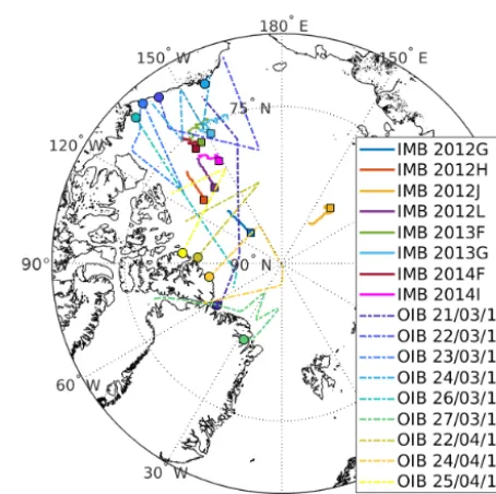
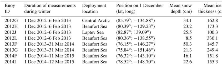
IMBs are installed by the Cold Regions Research and En-gineering Laboratory (CRREL) to measure the ice mass bal-ance of the Arctic sea ice cover (Richter-Menge et al., 2006; Perovich and Richter-Menge, 2006). Buoy components in-clude acoustic sounders and a string of thermistors. The ther-mistor string extends from the air, through the snow cover and sea ice, into the water and has temperature sensors lo-cated every 10 cm along the string. It measures the physical temperature with an accuracy of 0.1 K. There are two acous-tic sounders located above the snow surface and below the sea ice. The acoustic sounders measure the position of snow and ice surfaces (top and bottom) with a precision of 5 mm, from which the snow depth is computed. The buoys also in-clude instruments that measure air temperature, barometric air pressure, and GPS geographical position (Perovich et al., 2019). Several IMBs are deployed by the CRREL at different locations and times during the year. We only use Arctic buoy data recorded during winter (1 December to 1 April) to avoid cases where ice starts to melt. The IMBs available for this study are all located on MYI, with an ice thickness≥1 m. A summary of buoy information corresponding to these criteria is given in Table 1 and the IMB locations are shown in Fig. 1. IMB measurements collocated with AMSR2 TBs used in this study totalize 2845 observations.
For snow depth retrieval, we also used data from the OIB airborne campaign. The NASA OIB project has collected ice and snow depth data in the Arctic during annual flight campaigns (March–May) since 2009. The data are especially valuable in this context, since they contain snow depth in-formation from the snow radar on board the aircraft, not only from single points but continuously along the flight path. The
Figure 1.Ice mass balance buoy and Operation Ice Bridge (OIB) flight locations over Arctic sea ice. Squares indicate the position of IMBs on 1 December and circles indicate the starting points of the OIB campaigns.
vertical resolution of the OIB snow radar is 3 cm, and the un-certainty on the snow depth is around 6 cm compared with in situ measurements (Kurtz et al., 2013). Recent studies evi-dence larger errors on OIB snow depth (Kwok and Maksym, 2014) with issues to detect snow depth under 8 cm (Kwok and Maksym, 2014; Holt et al., 2015). These different limi-tations are summarized in Kwok et al. (2017). In the RRDP, the snow depth data from OIB snow radar are averaged into 50 km sections to be collocated with AMSR2 observations. For our study we use the OIB data from the 2013 campaign. It totalizes 408 observations over 8 d in March and April and covers FYI and MYI areas. Figure 1 summarizes the loca-tions of IMBs and OIB campaigns over the Arctic ocean.
It is important to note that there are discrepancies due to the scale when comparing point measurements from buoys with the spatially averaged data from satellites or aircrafts (Dybkjær et al., 2012).
2.2 The database of simulated effective temperature and brightness temperature from sea ice properties
For the estimation of Teff, we use a microwave emission
model coupled with a thermodynamic model. The emission model uses the temperature, density, snow crystal and brine inclusion size, salinity, and snow or ice type to estimate the microwave emissivity, theTeff, and the TB of sea ice. It is
Table 1.List of the IMBs used in this study, with the mean snow depth (column 5) and the mean ice thickness (column 6) computed over the duration of the measurements (column 2).
Buoy Duration of measurements Deployment Position on 1 December Mean snow Mean ice
ID during winter location (lat, long) depth (cm) thickness (cm)
2012G 1 Dec 2012–6 Feb 2013 Central Arctic (85.79◦;−134.88◦) 34.1 162.8 2012H 1 Dec 2012–6 Feb 2013 Beaufort Sea (80.39◦;−129.23◦) 23.2 173.3 2012J 1 Dec 2012–6 Feb 2013 Laptev Sea (82.87◦; 139.09◦) 25.5 100.3 2012L 1 Dec 2012–6 Feb 2013 Beaufort Sea (80.36◦;−138.55◦) 8.5 330.1 2013F 1 Dec 2013–31 Mar 2014 Beaufort Sea (76.15◦;−146.27◦) 50.3 145.7 2013G 1 Dec 2013–31 Mar 2014 Beaufort Sea (75.84◦;−151.46◦) 21.3 249.4 2014F 1 Dec 2014–11 Mar 2015 Beaufort Sea (76.32◦;−143.10◦) 16.1 151.8 2014I 1 Dec 2014–12 Mar 2015 Beaufort Sea (78.52◦;−148.70◦) 22.6 155.3
wind speed, incoming shortwave and longwave radiation, rel-ative humidity, and accumulated precipitation. It computes a centimetre-scale profile of the parameters used as inputs to the emission model. The emission model used here is a sea ice version of the Microwave Emission Model of Lay-ered Snowpacks (MEMLS) (Wiesmann and Mätzler, 1999) described in Mätzler (2006). The simulations were part of an earlier version of the RRDP and the simulation methodol-ogy is described in Tonboe (2010). This MEMLS simulation uses, among its inputs, the snow depth and theTSnow−Iceand
computesTeffsand TBs at different frequencies (from 1.4 to
183 GHz). The data set contains 1100 cases and is called the MEMLS-simulated data set in the following.
2.3 Methodology
In this study, we propose simple algorithms, using multilin-ear regressions, to derive the snow depth, theTSnow−Ice, and
theTeffof sea ice from AMSR2 TBs.
The measurements from the IMB 2012G, 2012H, 2012J, and 2012L, collocated with AMSR2 TBs, are used as the training data set for the different regressions to retrieve snow depth andTSnow−Ice. These buoys have been selected because
they are located in different regions across the Arctic and show a large range of snow depths. The measurements from IMB 2013F, 2013G, 2014F, and 2014I, which are all located in the Beaufort Sea, are used as the testing data set.
First, the IMB snow depth is expressed as a function of the AMSR2 TBs using a multilinear regression (see Sect. 3.1). The OIB data are used for the forward selection and the IMB training data set is used to perform the regression. Second, the TSnow−Ice is expressed as a function of TBs and snow
depth, using linear regressions. An automated method is de-veloped that detects the position of the snow–ice interface on the vertical temperature profile measured by the IMB ther-mistor string (see Sect. 4.1). Then, the IMB training data set is used to perform the regressions (see Sect. 4.3). For this part there are two consecutive regressions: the first one is done be-tween the centred (the average was subtracted)TSnow−Iceand
TBs; the second one is done between theTSnow−Icecorrected
for the TB dependence and the snow depth. Third, the sea iceTeff at different microwave frequencies is expressed as a
function of theTSnow−Ice(see Sect. 5.2). This final step uses
the simulations from a thermodynamical model and MEMLS to derive linear regression equations for theTeff at
frequen-cies between 6 and 89 GHz. TheTeffat 50 GHz is of special
interest for atmospheric sounding applications.
3 Snow depth estimation
3.1 Multilinear regression to retrieve the snow depth A forward selection method is used to choose the best AMSR2 channels to retrieve snow depth. It is a statistical method to determine the best-predictor combinations (here, AMSR2 TBs) to retrieve a variable (here, snow depth). We use the stepwise regression (Draper and Smith, 1998). It is a sequential predictor selection technique: at each step statistic tests are computed, and the predictors included in the model are adjusted. Our training data set for this forward selection is the OIB snow depth from the 2013 campaign included in the RRDP. OIB data are chosen for forward selection because the data cover a large area with a wide range of snow depths. In addition, the scale of the averaged OIB data is closer to satel-lite footprint than buoy measurements, increasing the consis-tency with the satellite observations. Forward selection tests have also been done with the IMB training data set, but the results were not satisfactory. We find that the best channel combination for snow depth retrieval is the combination of the three channels at 6.9, 18.7, and 36.5 GHz in vertical po-larization (6, 18, and 36 V).
Then, a multilinear regression is conducted using the IMB training data set (buoys G, H, J, L in 2012 collocated with AMSR2 TBs). The snow depth is given as a linear combina-tion of the TBs at 6, 18, and 36 V:
Ds=1.7701+0.0175·TB6 V−0.0280·TB18 V
withDsthe snow depth expressed in metres and TB in kelvin.
This model was trained with snow depths between 5 and 40 cm.
The forward selection has also been tested by constrain-ing the number of predictors to 2 and 4. The combinations obtained are 18 and 36 V for two channels and 6, 18, 36, and 89 V for four channels. Then, the multilinear regression has been performed using these combinations of two or four channels. The results show that the three-channel combina-tion is the best in terms of RMSE and correlacombina-tion compared to the two- or four-channel combination (see Sect. 3.2). 3.2 Results of the snow depth retrieval
Figure 2 shows the comparison between the observed snow depth measured by the acoustic sounder of IMB and the regressed snow depth computed from AMSR2 TBs with Eq. (2). The RMSE between the IMB snow depth observa-tions and our snow depth regression is 12.0 cm and the cor-relation coefficient is 0.66, using the IMBs 2013F, 2013G, 2014F, and 2014I (which are not in the training data set). The buoy 2013F observes a large snow depth (>40 cm), which is outside the bounds of our snow depth model. Tests are con-ducted to improve the estimation, including the 2013F buoy in the training data set, with equal numbers of observations for different ranges of snow depths: it does not improve the results. Our model obtained the same snow depth estimation between buoys 2013G and 2013F. It is consistent because these buoys are spatially very close. Therefore, we suspect that the 2013F buoy is located nearby a ridge or hummock, where the local snow depth is large but not detectable at the satellite footprint scale. Without including the buoy 2013F in the computation, the RMSE for our snow depth model is 5.1 cm and the correlation coefficient is 0.61.
We also compare the snow depth retrievals with the mea-surements of the 2013 OIB campaigns (see Fig. 3) with the ice type computed from the gradient ratio between 19 and 37 GHz (Baordo and Geer, 2015). Our snow depth regression (Eq. 2) RMSE is 6.26 cm and the correlation coefficient with OIB observations is 0.87. Note that the uncertainties on OIB data for the 2013 campaigns are between 2 and 22 cm with a mean standard deviation (SD) of 11 cm (OIB snow depth Dsnow provided in the RRDP). Looking at Fig. 3, our snow depth regression is applicable to both ice types. The RMSEs computed for MYI and FYI are 7.2 and 3.9 cm, and the cor-relations are 0.71 and 0.03. The RMSE is smaller for FYI be-cause the snow depth variability of FYI is also smaller. The low correlation obtained for FYI can come from the limited number of observations and because the snow depth variabil-ity observed is within the signal noise.
Spatial scales are different when comparing satellite mea-surements or airborne campaign meamea-surements with buoy measurements. Discrepancies can appear due to the spatial variability of the snow depth. It can explain that the cor-relation is higher when comparing snow depth estimated
from AMSR2 TBs with the snow depth observed from OIB radar. It is also important to note that the OIB campaign data are from late winter to beginning of spring (March to April), while IMB measurements are from winter (Decem-ber to March). With the snow depth regression being devel-oped on IMB measurements, this small change in season can contribute to the larger RMSE observed with OIB data.
4 Snow–ice interface temperature estimation 4.1 Automatic interface position detection
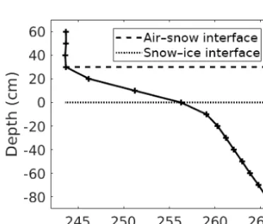
During winter, the air temperature is very cold, meaning that the snow surface temperature is cold compared to ice and water temperatures. Through sea ice, the temperature profile is piecewise linear and temperature increases with depth (see Fig. 4). In the air, the temperature gradient is small because of turbulent mixing. In the snow, the temperature gradient is larger due to the thermal properties of snow. Therefore, air– snow and snow–ice interface positions can be detected by changes in the temperature gradient. At the air–snow inter-face, the second derivative of the temperature profile reaches a maximum. At the snow–ice interface, the temperature gra-dient being lower in the ice than in the snow, the second derivative of the temperature profile reaches a minimum. Us-ing these properties of the sea ice temperature profile, an au-tomated method is implemented to detect the air–snow and the snow–ice interface positions in the temperature profile measured by the buoy thermistor string.
Figure 4 shows an averaged temperature profile through sea ice during winter, with the air–snow and snow–ice in-terface positions detected with our automated method. This method performs best during winter when the air is cold. It may not be applicable if the snow depth is lower than the ver-tical resolution of the thermistor string (10 cm) or if sea ice starts to melt and the temperature profile develops gradually toward an isothermal state. The method selects the thermis-tor which is located the closest to the interface. Note that the real interface position can be located between two thermis-tors. Therefore, the shift between the real interface position and the thermistor the closest to the interface can be up to 5 cm. This can introduce uncertainties in ourTSnow−Ice
re-gression.
4.2 Correlation between the brightness temperature and the snow–ice interface temperature
Figure 2.Time series of the comparison between snow depths from IMB observations and our multilinear regression (Eq. 2). The beginning of the measurements with a new IMB is indicated on thexaxis.
Figure 3.Time series of the comparison between snow depths (leftyaxis) from OIB observations and our multilinear regression (Eq. 2). The beginning of the measurements with a new OIB campaign is indicated on thexaxis. For each measurement, the ice type is indicated with a dashed grey line (rightyaxis).
Figure 4.Averaged temperature profile (from December to Febru-ary) measured by the IMB 2012G, with air–snow and snow–ice in-terface levels detected with our automated method.
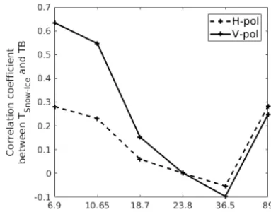
We use a correlation analysis to select the TBs at differ-ent frequencies describing the variability of the TSnow−Ice.
Figure 5 shows the correlation coefficient betweenTSnow−Ice
and AMSR2 TBs computed using the data from all IMBs (Table 1). The 89 GHz TBs are highly correlated with the air
temperature (R >0.75). The 18.7, 23.8, and the 36.5 GHz TBs have a low correlation withTSnow−Ice because of
mi-crowave scattering in the snow and/or shallow mimi-crowave penetration into the snow. The 7.3 GHz channel is ignored because it contains practically the same information as the 6.9 GHz channel. The TBs at 6.9 and 10.65 GHz at verti-cal polarization have the highest correlation withTSnow−Ice
(R >0.5). Therefore, the 10.65 and the 6.9 GHz at vertical polarization (10 and 6 V) channels are selected as inputs to the linear regression to retrieve theTSnow−Ice.
4.3 Linear regressions to retrieve the snow–ice interface temperature
To express theTSnow−Ice as a function of the TB at 6 and
10 V, the linear regressions are calculated on centred data (i.e. the anomaly). For each buoy, the averagedTSnow−Iceis
subtracted from theTSnow−Icemeasurements and the same is
done with the TB measurements. Thus, the temperature off-set between the buoys is removed and the slope of the linear regression is unchanged:
1TSnow−Ice=a1·1TB6 or 10 V⇔TSnow−Ice
Figure 5.Correlation coefficient between theTSnow−Icefrom IMBs and the AMSR2 TBs, as a function of AMSR2 frequency.
with1TSnow−Iceand1TB describing the centredTSnow−Ice
and TB. Figure 6 shows the linear regression between the TSnow−Iceand the TB at 6 and 10 V, using the measurements
from buoys 2012G, 2012H, 2012J, and 2012L. The slope co-efficients (a1) estimated between theTSnow−Iceand the TB at
6 and 10 V are 1.086±0.020 and 1.078±0.019.
The offset (offsetbuoy) in the linear regression equations
betweenTSnow−Iceand the TB is different for each buoy,
be-cause it depends on the snow depth. The TSnow−Ice
depen-dence on snow depth can be explained by the thermal insu-lation of snow (Maaß et al., 2013; Untersteiner, 1986). Here, we establish an empirical relationship between theTSnow−Ice
corrected for the TB linear dependence at 10 or 6 V, and the snow depth as follows:
TSnow−Ice−a1·TB10 or 6 V=a2·f (Ds)+a3, (4)
withf (Ds)a function of snow depth.
Three different linear regressions have been tested to relate theTSnow−Iceusing the snow depth directly, the inverse of the
snow depth, and the logarithm of snow depth. Figure 7 shows the TSnow−Ice corrected from TB dependence as a function
of snow depth. The different regressions are tested using the training data set (IMB G, H, J, and L in 2012). The regression showing the best results uses the logarithm of the snow depth (solid black line in Fig. 7). The linear regression using the snow depth directly (dashed red line in Fig. 7) leads to an overestimation of the TSnow−Ice for large snow depth. The
regression using the inverse of the snow depth (red dotted line in Fig. 7) leads to an underestimation for small snow depth. The RMSEs obtained on theTSnow−Iceare compared
and the relation using the logarithm of snow depth shows the lowest RMSE. Based on these results, the final equations to relate theTSnow−Iceto the snow depth and the TB at 10 and
at 6 V are as follows:
TSnow−Ice=1.078·TB10 V+5.67·log(Ds)−5.13 (5)
TSnow−Ice=1.086·TB6 V+3.98·log(Ds)−10.70, (6)
whereTSnow−Iceand TB are expressed in kelvin, andDs is
expressed in metres.
4.4 Results of the snow–ice interface temperature retrieval
Figure 8 shows the comparisons between the observed TSnow−Ice and the regressedTSnow−Iceusing the 10 and 6 V
TBs (Eqs. 5 and 6), and the in situ snow depth measured by the acoustic sounder of IMB. The RMSEs are computed using the IMB 2013F, 2013G, 2014F, and 2014I. The regres-sion of theTSnow−Ice using the in situ snow depth with the
10 V TBs (Eq. 5) is slightly better (RMSE=1.78 K) than the regression with the 6 V TBs (Eq. 6) (RMSE=1.98 K). The variability due to the snow depth is better described with the regression using the 10 V TBs. Figure 9 is the same as Fig. 8 but with our snow depth estimation (Eq. 2). The RM-SEs are 2.87 K for the 10 V regression and 2.90 K for the 6 V regression. The results are degraded because of the snow depth regression, especially for the buoys with thick snow (∼50 cm) or thin snow (∼5 cm) (e.g. buoy 2013F and buoy 2012L). Note that the regression is tested with IMBs, which are all located on MYI. However, using our algorithm to de-rive theTSnow−Ice is also applicable over FYI areas, as our
snow depth algorithm is applicable to both ice types and ourTSnow−Icealgorithm uses the channels 10 or 6 V, which
have limited sensitivity to the ice type (Comiso, 1983; Spreen et al., 2008).
5 Sea ice effective temperature estimation 5.1 Bias between the model and the observations Teffis related to the frequency and the incidence angle of the
satellite observations. It is not a geophysical variable that we can measure directly as an in situ parameter. A microwave emission model has to be used to computed theTeffsfrom the
geophysical parameters. TheTeffused here is available from
a simulated data set using a thermodynamical model and the microwave emission model, MEMLS. The model set-up and the simulations are described in Tonboe (2010). In this data set, the TBs and theTeffs are simulated using theTSnow−Ice
and the input snow and ice profiles from the thermodynami-cal model. Even though the simulated TB data are compara-ble to observations in terms of mean and standard deviation, both the thermodynamical model and the emission model are based on physical equations and are not tuned to observa-tions. TBs simulated with MEMLS are not fitted to AMSR2 TBs, meaning that a bias is expected between theTSnow−Ice
of the MEMLS-simulated data set (TSnow-Ice MEMLS) and the
Figure 6.CentredTSnow−Iceexpressed as a function of the centred TBs at 10 V(a)and 6 V(b). Data from the IMBs are in different colours depending on the buoy, and the linear regression is the solid black line.
Figure 7.TSnow−Icecorrected for the 10 V TB(a)and of the 6 V TB(b)dependence as a function of snow depth. Data from the IMBs are represented by different colours, the regression using the snow depth is shown by the dashed red line, the regression using the inverse of snow depth by the dotted red line, and the regression using the logarithm of the snow depth by the solid black line.
The bias obtained is the mean value of the difference be-tween theTSnow-Ice MEMLS, and theTSnow−Iceregressed from
Eqs. (5) and (6) using the TBs of the MEMLS-simulated data set as inputs. Biases of 3.97 and 4.01 K are estimated for the regressions with 10 and 6 V respectively. The RMSEs computed between theTSnow-Ice MEMLSand theTSnow−Ice
re-gressed and corrected for the biases at 10 and 6 V are 2.7 and 2.07 K.
Figure 10 shows the TSnow−Ice from the
MEMLS-simulated data set as a function of TB at 10 and 6 V, and the TSnow−Icecomputed from our regressions (Eqs. 5 and 6), with
and without the bias correction. We can see that the slopes of our linear regressions are consistent with the data simulated from MEMLS.
5.2 Linear regression between the effective temperature and the snow–ice interface temperature
The Teff near 50 GHz in vertical polarization is correlated
with theTSnow−Ice (Tonboe et al., 2011) and it can be
ex-pressed as a linear function of theTSnow−Ice:
Teff(freq,pol)=b1(freq,pol)·TSnow-Ice MEMLS+b2(freq,pol), (7) withTeff,b1, andb2depending on the frequency (freq) and
on the polarization (pol). We use the MEMLS-simulated data set to calculate the linear regression between theTSnow−Ice
and theTeff at 6.9, 10.65, 18.7, 23.8, 36.5, 50, and 89 GHz
in vertical polarization.Teffsat vertical and horizontal
Figure 8.Time series of the comparisons betweenTSnow−Iceobservations from IMBs (black line), andTSnow−Iceregressions with TBs at 10 V (blue line) and at 6 V (red line). The snow depth used in Eqs. (5) and (6) is the snow depth observed by the IMB sounder. The beginning of the measurements with a new IMB is indicated on thexaxis.
Figure 9.Same as Fig. 8, using the regressed snow depth (Eq. 2) in place of in situ snow depth
horizontal polarization due to the variability of sea ice emis-sivity at this polarization.
Figure 11 shows theTeffat 50 V as a function ofTSnow−Ice.
The linear regressions between theTSnow−Iceand theTeffat
different frequencies are computed. The coefficients b1and
b2of Eq. (7) are given in Table 2. The slope coefficient of the
regression increases with frequency, meaning that the sen-sitivity of the Teff to the TSnow−Ice is increasing with
fre-quency between 6 and 89 GHz. A slope coefficient lower than 1 means that the penetration depth at the given frequency is deeper than snow–ice interface. At 50 GHz the slope coeffi-cient is near to 1, meaning that the penetration depth is close to the depth of the snow–ice interface. The RMSEs are be-low 1 K, with the regression ofTeffat 50 V showing the
low-est RMSE (0.33 K), and at 89 V showing the highlow-est RMSE (0.92 K).
These linear regressions between the Teff and the
TSnow-Ice MEMLS(Eq. 7) are the final step in retrieving theTeff
of sea ice at microwave frequencies as a function of TBs, us-ing the work in the previous sections to express theTSnow−Ice
as a function of TBs (Eqs. 2, and 5 or 6). The biases be-tween the AMSR2 observations and the MEMLS-simulated
Table 2.Regressions of theTefffor different frequencies at vertical polarization as a function of theTSnow−Ice (see Eq. 7) using the MEMLS-simulated data set.
Frequency Slope Offset RMSE
(GHz) coefficient (K) (K)
b1 b2
6.9 0.888 30.2 0.89
10.7 0.901 26.6 0.75
18.7 0.920 21.5 0.63
23.8 0.932 18.4 0.57
36.5 0.960 10.9 0.41
50 0.989 2.96 0.33
89 1.06 −16.4 0.92
data set are taken into account, replacingTSnow-Ice MEMLSby
TSnow−Iceestimated from AMSR2 TBs with a bias correction
(see Table 2):
Figure 10.Comparisons between theTSnow-Ice MEMLSfrom the MEMLS-simulated data is shown with blue points, the regressedTSnow−Ice (Eqs. 5 and 6) with a dashed black line, and the regressedTSnow−Icedebiased to fit the MEMLS simulations with a solid black line at 10 V(a) and 6 V(b)channels.
Figure 11. Regression of the Teff as a function ofTSnow−Ice at 50 GHz in vertical polarization. The data from the MEMLS simu-lations are in blue points and the linear regression is the solid black line.
Teff(freq,pol)=b1(freq,pol)·(TSnow−Ice−4.01)+b2(freq,pol), for the regression using 6 V TB. (9)
6 Discussion
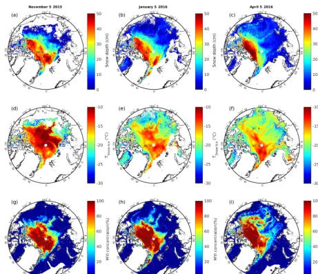
For days in November, January, and April, Fig. 12 shows the maps of the snow depth estimated with our multilinear re-gression (Eq. 2), theTSnow−Iceestimated with our multilinear
regression (Eq. 5), and the MYI concentration products from the University of Bremen (https://seaice.uni-bremen.de, last access: 1 November 2018). Maps of the MYI concentra-tion from University of Bremen are derived from AMSR2 and from the Advanced SCATterometer (ASCAT) with the method of Ye et al. (2016a, b). To perform our regressions,
we use the AMSR2 TBs (Level L1R) provided by JAXA and the SIC from the European Centre for Medium-Range Weather Forecasts (ECMWF) Reanalysis Interim (ERA-Interim) data. Only the areas with 100 % SIC are considered to compute the snow depth on sea ice and theTSnow−Icewith
our method.
The results show that the snow depth is larger (40 cm) in the north of Greenland (Warren et al., 1999; Shalina and Sandven, 2018) due to the presence of drift snow caused by the numerous pressure ridges present in this area (Hanson, 1980), as anticipated. We can observe that the snow depth is larger in areas with larger MYI concentrations. The variabil-ity of the snow cover is low during winter, as the snow depth reaches a maximum by December and remains relatively un-changed until snowmelt (Sturm et al., 2002).
ForTSnow−Ice, in January and April when the air
tempera-ture is cold (between−20 and−30◦C over the whole Arctic, on 5 January and 5 April 2016 from ERA-Interim air temper-ature), the areas with large snow depth show largerTSnow−Ice
because of the thermal insulation power of the snow. It is dif-ferent in November: the air temperature is warmer (∼ −5◦C near Kara Sea,∼ −15◦C near Laptev Sea, and∼ −25◦C in the central Arctic and Beaufort seas, on 5 November 2015 from ERA-Interim air temperature) and the areas with thin-ner snow show larger TSnow−Ice which are close to the air
temperature (Perovich and Elder, 2001). Note that we can observe lowTSnow−Icein some locations near the sea ice
mar-gins due to the presence of open ocean in the satellite foot-print. As the brightness temperature of open water is low, the total brightness temperature measured is decreased and it impacts ourTSnow−Iceestimation.
Visually theTSnow−Iceshows a high correlation with the
Figure 12.Maps of the snow depth(a, b, c)and theTSnow−Ice(d, e, f)estimated from our multilinear regression using AMSR2 TBs, with multi-year ice (MYI) concentration products(g, h, i)from the University of Bremen on 5 November 2015(a, d, g), 5 January 2016(b, e, h), and 5 April 2016(c, f, i).
coast, marking the Beaufort Gyre of the Arctic sea ice drift (see the animations for the same year at https://seaice. uni-bremen.de/multiyear-ice-concentration/animations/, last access: 1 November 2018). The main differences between FYI and MYI are, on average, the higher thickness of MYI and its higher snow load. Both effects will influence the TSnow−Ice. Under the same conditions, a higher ice thickness
will lead to a lower TSnow−Ice. In contrast, it will be higher
if only the snow depth is increased. The positive correlation between MYI concentration andTSnow−Icesuggests that the
influence of the higher snow depth on MYI outbalances that of the higher ice thickness on theTSnow−Ice, emphasizing the
important role of snow on sea ice in its thermodynamic bal-ance.
The similar patterns observed between the maps of the TSnow−Iceand the MYI concentration on Fig. 12 are
encour-aging and give confidence in the methodology developed here, as these MYI concentration products are from indepen-dent work done at the University of Bremen and distributed daily to users. However it should be noted that the input chan-nels of both methods overlap in some AMSR2 chanchan-nels, and even different channels show some covariance (Scarlat et al., 2017).
7 Conclusions
We derive simple algorithms to estimate sea ice parameters such as the snow depth, theTSnow−Ice, and theTeffof sea ice
are used for the regression of theTeff. All the equations used
to retrieve these sea ice parameters are derived using several linear and multilinear regressions.
Our regression to retrieve the snow depth over winter Arc-tic sea ice uses the TBs at 6.9, 18.7, and 36.5 GHz in verti-cal polarization. A RMSE of 5.1 cm is obtained between the estimated and the IMB snow depths using an independent IMB test data set. This snow depth retrieval is applicable to FYI and MYI, with lower uncertainties for FYI than for MYI (3.9 cm compared to 7.2 cm). To retrieve theTSnow−Ice, two
relations are derived using two different AMSR2 channels (10 or 6 V) and the estimated snow depth. The two regres-sions show similar results. The errors are 2.87 and 2.90 K at 10 and 6 V. ThisTSnow−Iceretrieval has been tested only for
MYI. It can also be applied to FYI, as the 6 and 10 V chan-nels have limited sensitivity to the ice type (Comiso, 1983; Spreen et al., 2008). Finally theTeffsat 6.9, 10.65, 18.7, 23.8,
36.5, 50, and 89 GHz in vertical polarization are retrieved as a function ofTSnow−Iceusing linear regressions. At the final
step, the RMSEs of the linear regressions between the sim-ulatedTSnow−Iceand theTefffor all channels are lower than
1 K, with a minimum value of 0.33 K at 50 GHz, which is a key frequency for atmosphere temperature retrieval. The methodology used to estimate snow depth andTSnow−Icehas
been applied to several days during winter. It shows consis-tent results with MYI concentration estimates obtained inde-pendently.
These algorithms can be used to create snow depth and TSnow−Ice products which can improve the study of sea ice
variability (e.g. sea ice growth). Information on theTSnow−Ice
may help in sea ice models by constraining the sea ice tem-perature gradient and the thermodynamical ice growth. The Teffestimations can be used in atmospheric radiative transfer
calculations and to reduce noise in SIC retrieval algorithms (Tonboe et al., 2013) (e.g. EUMETSAT OSISAF global SIC product).
Data availability. The round robin data package used for this study is publicly accessible at https://figshare.com/articles/Reference_ dataset_for_sea_ice_concentration/6626549 (Pedersen et al., 2018).
Author contributions. This study was conducted by LK and super-vised by RTT and CP. GH contributed to the analysis and to the correction of the draft.
Competing interests. The authors declare that they have no conflict of interest.
Acknowledgements. This research was funded by EUMETSAT OS-ISAF (OSI VS17 03) and the PNTS (Programme national de télédédtection spatiale). The authors acknowledge the support from the EUMETSAT OSISAF visiting scientist programme and the
Danish Meteorological Institute for its welcome. We also acknowl-edge the reviewers for their precious comments, which improved this manuscript a lot.
Review statement. This paper was edited by John Yackel and re-viewed by Leif Toudal Pedersen and one anonymous referee.
References
Baordo, F. and Geer, A.: Microwave Surface Emissivity over sea-ice, EUMETSAF NWP SAF, Tech. Rep. NWP-SAF_EC_VS_026, 1–30, 2015.
Comiso, J.: Sea ice effective microwave emissivities from satellite passive microwave and infrared observations, J. Geophys. Res., 88, 7686–7704, 1983.
Comiso, J., Cavalieri, D., and Markus, T.: Sea ice concentration, ice temperature, and snow depth using AMSR-E data, IEEE T. Geosci. Remote, 41, 243–252, 2003.
Draper, N. R. and Smith, H.: Applied regression analysis, John Wi-ley & Sons, Inc., Hoboken, NJ, USA, 1998.
Dybkjær, G., Tonboe, R., and Høyer, J. L.: Arctic surface temper-atures from Metop AVHRR compared to in situ ocean and land data, Ocean Sci., 8, 959–970, https://doi.org/10.5194/os-8-959-2012, 2012.
English, S. J.: The Importance of Accurate Skin Temperature in As-similating Radiances From Satellite Sounding Instruments, IEEE T. Geosci. Remote, 46, 403–408, 2008.
Fichefet, T. and Maqueda, M. A. M.: Modelling the influence of snow accumulation and snow-ice formation on the seasonal cycle of the Antarctic sea-ice cover, Clim. Dynam., 15, 251–268, 1999. Grönfeldt, I.: Snow and sea ice temperature profiles from satellite data and ice mass balance buoys, Lund University, Sweden, Tech. rep., 370, 1–72, 2015.
Hall, A.: The role of surface albedo feedback in climate, J. Climate, 17, 1550–1568, 2004.
Hanson, A. M.: The Snow Cover of Sea Ice during the Arctic Ice Dynamics Joint Experiment, 1975 to 1976, Arctic Alpine Res., 12, 215–226, https://doi.org/10.1080/00040851.1980.12004180, 1980.
Harlow, R.: Millimeter Microwave Emissivities and Effective Tem-peratures of Snow-Covered Surfaces: Evidence for Lambertian Surface Scattering, IEEE T. Geosci. Remote, 47, 1957–1970, 2009.
Harlow, R. C.: Sea Ice Emissivities and Effective Temperatures at MHS Frequencies: An Analysis of Airborne Microwave Data Measured During Two Arctic Campaigns, IEEE T. Geosci. Re-mote, 49, 1223–1237, 2011.
Holt, B., Johnson, M. P., Perkovic-Martin, D., and Panzer, B.: Snow depth on Arctic sea ice derived from radar: In situ comparisons and time series analysis, J. Geophys. Res.-Oceans, 120, 4260– 4287, 2015.
Kern, S. and Ozsoy-Çiçek, B.: Satellite remote sensing of snow depth on Antarctic Sea Ice: An inter-comparison of two empirical approaches, Remote Sensing, 8, 450, https://doi.org/10.3390/rs8060450, 2016.
ice thickness, freeboard, and snow depth products from Oper-ation IceBridge airborne data, The Cryosphere, 7, 1035–1056, https://doi.org/10.5194/tc-7-1035-2013, 2013.
Kwok, R. and Maksym, T.: Snow depth of the Weddell and Belling-shausen sea ice covers from IceBridge surveys in 2010 and 2011: An examination, J. Geophys. Res.-Oceans, 119, 4141– 4167, 2014.
Kwok, R., Kurtz, N. T., Brucker, L., Ivanoff, A., Newman, T., Farrell, S. L., King, J., Howell, S., Webster, M. A., Paden, J., Leuschen, C., MacGregor, J. A., Richter-Menge, J., Harbeck, J., and Tschudi, M.: Intercomparison of snow depth retrievals over Arctic sea ice from radar data acquired by Operation IceBridge, The Cryosphere, 11, 2571–2593, https://doi.org/10.5194/tc-11-2571-2017, 2017.
Lecomte, O., Fichefet, T., Vancoppenolle, M., and Nico-laus, M.: A new snow thermodynamic scheme for large-scale sea-ice models, Ann. Glaciol., 52, 337–346, https://doi.org/10.3189/172756411795931453, 2011.
Maaß, N., Kaleschke, L., Tian-Kunze, X., and Drusch, M.: Snow thickness retrieval over thick Arctic sea ice using SMOS satellite data, The Cryosphere, 7, 1971–1989, https://doi.org/10.5194/tc-7-1971-2013, 2013.
Maeda, T., Imaoka, K., Kachi, M., Fujii, H., Shibata, A., Naoki, K., Kasahara, M., Ito, N., Nakagawa, K., and Oki, T.: Sta-tus of GCOM-W1/AMSR2 development, algorithms, and prod-ucts, in: Sensors, Systems, and Next-Generation Satellites XV, SPIE Remote Sensing, 2011, Prague, Czech Republic, edited by: Meynart, R., Neeck, S. P., and Shimoda, H., SPIE, 8176, https://doi.org/10.1117/12.898381, 2011.
Maeda, T., Taniguchi, Y., and Imaoka, K.: GCOM-W1 AMSR2 level 1R product: Dataset of brightness temperature modified us-ing the antenna pattern matchus-ing technique, IEEE T. Geosci. Re-mote, 54, 770–782, 2016.
Markus, T. and Cavalieri, D. J.: Snow Depth Distribution Over Sea Ice in the Southern Ocean from Satellite Passive Microwave Data, in: Antarctic Sea Ice: Physical Processes, Interactions and Variability, edited by: Jeffries, M. O., American Geophysical Union, Washington, DC, 19–39, 1998.
Markus, T., Massom, R., Worby, A., Lytle, V., Kurtz, N., and Maksym, T.: Freeboard, snow depth and sea-ice roughness in East Antarctica from in situ and multiple satellite data, Ann. Glaciol., 52, 242–248, 2011.
Mathew, N., Heygster, G., Melsheimer, C., and Kaleschke, L.: Sur-face Emissivity of Arctic Sea Ice at AMSU Window Frequencies, IEEE T. Geosci. Remote, 46, 2298–2306, 2008.
Mätzler, C.: Thermal microwave radiation applications for remote sensing, Institution of Engineering and Technology, London, UK, 2006.
Maykut, G. A. and Untersteiner, N.: Some results from a time-dependent thermodynamic model of sea ice, J. Geophys. Res., 76, 1550–1575, https://doi.org/10.1029/JC076i006p01550, 1971.
Pedersen, L. F. and Saldo, R.: Sea Ice Concentration (SIC) Round Robin Data Package, Sea Ice Climate Initiative: Phase 2, ESA, Tech. Rep. SICCI-RRDP-07-16 Version: 1.4, 2016.
Pedersen, L. T., Saldo, R., Ivanova, N., Kern, S., Heygster, G., Ton-boe, R., Huntemann, M., Ozsoy, B., Ardhuin, F., and Kaleschke, L.: Rasmus Reference dataset for sea ice concentration, Fileset, figshare, https://doi.org/10.6084/m9.figshare.6626549.v3, 2018.
Perovich, D. and Richter-Menge, J. A.: From points to Poles: ex-trapolating point measurements of sea-ice mass balance, Ann. Glaciol., 44, 188–192, 2006.
Perovich, D. K. and Elder, B. C.: Temporal evolution of Arctic sea-ice temperature, Ann. Glaciol., 33, 207–211, 2001.
Perovich, D., Richter-Menge, J., and Polashenski, C.: Observing and understanding climate change: Monitoring the mass bal-ance, motion, and thickness of Arctic sea ice, available at: http: //imb-crrel-dartmouth.org, last access: 17 April 2019.
Richter-Menge, J. A., Perovich, D. K., Elder, B. C., Claffey, K., Rigor, I., and Ortmeyer, M.: Ice mass-balance buoys: a tool for measuring and attributing changes in the thickness of the Arctic sea-ice cover, Ann. Glaciol., 44, 205–210, 2006.
Rosenkranz, P. W. and Mätzler, C.: Dependence of AMSU-A Brightness Temperatures on Scattering From Antarctic Firn and Correlation With Polarization of SSM/I Data, IEEE Geosci. Re-mote S., 5, 769–773, 2008.
Rostosky, P., Spreen, G., Farrell, S. L., Frost, T., Heygster, G., and Melsheimer, C.: Snow Depth Retrieval on Arctic Sea Ice From Passive Microwave Radiometers–Improvements and Extensions to Multiyear Ice Using Lower Frequencies, J. Geophys. Res.-Oceans, 123, 7120–7138, 2018.
Sato, K. and Inoue, J.: Comparison of Arctic sea ice thickness and snow depth estimates from CFSR with in situ observations, Clim. Dynam., 50, 289–301, 2018.
Scarlat, R. C., Heygster, G., and Pedersen, L. T.: Experiences with an Optimal estimation algorithm for surface and atmospheric pa-rameter retrieval from passive microwave data in the arctic, IEEE J. Sel. Top. Appl., 10, 3934–3947, 2017.
Shalina, E. V. and Sandven, S.: Snow depth on Arctic sea ice from historical in situ data, The Cryosphere, 12, 1867–1886, https://doi.org/10.5194/tc-12-1867-2018, 2018.
Spreen, G., Kaleschke, L., and Heygster, G.: Sea ice remote sens-ing ussens-ing AMSR-E 89-GHz channels, J. Geophys. Res., 113, C02S03, https://doi.org/10.1029/2005JC003384, 2008.
Sturm, M., Holmgren, J., and Perovich, D. K.: Winter snow cover on the sea ice of the Arctic Ocean at the Surface Heat Budget of the Arctic Ocean (SHEBA): Temporal evo-lution and spatial variability, J. Geophys. Res., 107, 8047, https://doi.org/10.1029/2000JC000400, 2002.
Tonboe, R. T.: The simulated sea ice thermal microwave emission at window and sounding frequencies, Tellus A, 62, 333–344, 2010. Tonboe, R. T., Dybkjær, G., and Høyer, J. L.: Simulations of the snow covered sea ice surface temperature and microwave effec-tive temperature, Tellus A, 63, 1028–1037, 2011.
Tonboe, R. T., Schyberg, H., Nielsen, E., Rune Larsen, K., and Tveter, F. T.: The EUMETSAT OSI SAF near 50 GHz sea ice emissivity model, Tellus A, 65, 18380, https://doi.org/10.3402/tellusa.v65i0.18380, 2013.
Untersteiner, N.: The geophysics of sea ice, Springer, Boston, Mas-sachusetts, 1986.
Warren, S. G., Rigor, I. G., Untersteiner, N., Radionov, V. F., Bryaz-gin, N. N., Aleksandrov, Y. I., and Colony, R.: Snow Depth on Arctic Sea Ice, J. Climate, 12, 1814–1829, 1999.
Wiesmann, A. and Mätzler, C.: Microwave Emission Model of Lay-ered Snowpacks, Remote Sens. Environ., 70, 307–316, 1999.
Ye, Y., Heygster, G., and Shokr, M.: Improving Multiyear Ice Con-centration Estimates With Reanalysis Air Temperatures, IEEE T. Geosci. Remote, 54, 2602–2614, 2016a.