www.nonlin-processes-geophys.net/20/883/2013/ doi:10.5194/npg-20-883-2013
© Author(s) 2013. CC Attribution 3.0 License.
Nonlinear Processes
in Geophysics
Hyperbolicity in temperature and flow fields during the formation of
a Loop Current ring
M. H. M. Sulman1,*, H. S. Huntley1, B. L. Lipphardt Jr.1, G. Jacobs2, P. Hogan2, and A. D. Kirwan Jr.1
1School of Marine Science and Policy, University of Delaware, Newark DE 19716, USA 2Naval Research Laboratory, Stennis Space Center, MS 39529, USA
*now at: Department of Mathematics and Statistics, Wright State University, 3640 Colonel Glenn Hwy.,
Dayton, OH 45435, USA
Correspondence to: A. D. Kirwan Jr. ([email protected])
Received: 3 June 2013 – Revised: 28 August 2013 – Accepted: 18 September 2013 – Published: 29 October 2013
Abstract. Loop Current rings (LCRs) are among the largest mesoscale eddies in the world ocean. They arise when bulges formed by the Loop Current in the Gulf of Mexico close off. The LCR formation process may take several weeks, and there may be several separations and reattachments be-fore final separation occurs. It is well established that this period is characterized by a persistent saddle point in the sea surface height field, as seen in both model and satellite data. We present here a detailed study of this saddle region during the formation of Eddy Franklin in 2010, over mul-tiple days and at several depths. Using a data-assimilating Gulf of Mexico implementation of the HYbrid Coordinate Ocean Model (HYCOM), we compare the vertical structure of the currents and temperature fields on 5 and 10 June 2010. Finite-time Lyapunov exponents (FTLE) are computed from the surface down to 200 m to estimate the location of relevant transport barriers. Several new features of the saddle region associated with LCR formation are revealed: the ridges in the FTLE fields are shown to be excellent surrogates for the manifolds delineating the material flow structures with only slight degradation at depth. The intersection of the ridges rep-resenting stable and unstable manifolds drops nearly verti-cally through the water column at both times; remarkably, the material boundary shapes are maintained even as they are advected. Moreover, velocity stagnation points and sad-dle points in the temperature field are consistently found near the intersections at all depths, and their geographic positions are also nearly constant with depth.
1 Introduction
The Yucatan–Florida current system, known as the Loop Current, is observed to be bimodal. In the retracted config-uration, the flow from the Yucatan enters the Gulf of Mex-ico, turns abruptly eastwards, and exits through the Florida Straits. In the extended configuration, the Loop Current pen-etrates northwards into the Gulf, forms a large anticyclonic loop, and then turns eastwards to exit the Gulf through the Straits of Florida. Occasionally, the loop pinches off to form a large anticyclonic mesoscale eddy or Loop Cur-rent ring (LCR). LCRs have velocities exceeding 1 m s−1
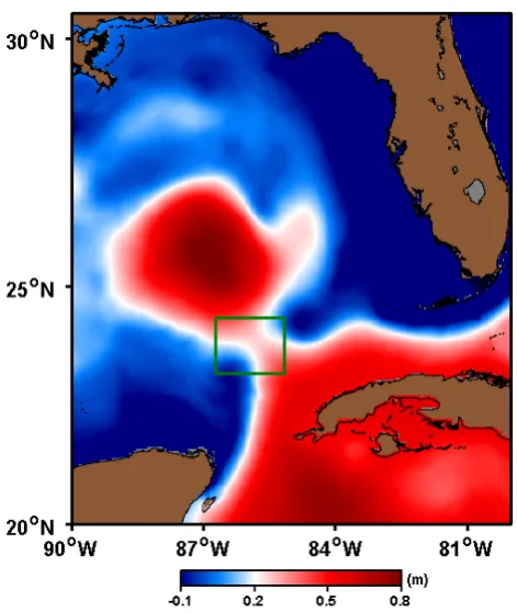
and may have diameters exceeding 200 km. Indest et al. (1989), Lewis et al. (1989), Forristall et al. (1992), and Glenn and Ebbesmeyer (1993) provided early comprehensive sum-maries of the characteristics of these structures. See Sturges et al. (2005) and Schmitz et al. (2005) for recent synopses of these features and their roles in the general circulation of the Gulf. Figure 1 gives an example of the sea surface height anomaly (SSHa) around the time of one LCR formation.
Fig. 1. Sea surface height anomaly (SSHa) of the Loop Current in
the Gulf of Mexico during a ring formation event on 10 June 2010. The saddle region in the small box is the focus of this study.
Peripheral cyclones are known to be contributing factors to the formation of LCRs (Chérubin et al., 2006; Schmitz, 2005; Oey et al., 2005). Less attention has been paid to the saddle structure character of the SSHa field. The premise of this study is that the hyperbolicity of the pinch-off region, such as the one shown in Fig. 1, rather than just the cyclonic components, is fundamental to LCR formation, since distin-guished material transport boundary surfaces are known to live in these regions. Support for this conjecture comes from the comprehensive analysis of Andrade-Canto et al. (2013), which showed these surfaces to be important LCR forma-tion diagnostics. It follows that detailed descripforma-tions of these two-dimensional material surfaces as they evolve in time are essential for improved understanding of the dynamical pro-cesses during the separation period. We also connect this La-grangian characterization with Eulerian snapshots of more easily observed quantities, in particular the temperature field. The analysis relies on a dynamical systems theory method-ology commonly called Lagrangian coherent structures (LCS). Nearly all LCS studies in geophysical fluid dynam-ics (GFD), and particularly oceanography, delineate mate-rial boundaries of adjacent vortices. Moreover, most analyses in oceanography are restricted to single layers at prescribed times. In reality, LCS are time-varying two-dimensional sur-faces embedded in a three-dimensional ocean. Thus, the first question addressed here is what is the time-evolving
three-dimensional picture of the LCS associated with the for-mation of a LCR?
Our focus is on the birth of Eddy Franklin in 2010. This event was extensively documented as it occurred during the Deepwater Horizon tragedy. Nonetheless, the exact date of eddy detachment is somewhat uncertain and dependent on the criteria applied. Published estimates range from late May 2010 to mid-June 2010 (Liu et al., 2011; Hamilton et al., 2011; Walker et al., 2011). Herein we consider the period 5– 10 June 2010.
In LCS theory, identification of “hyperbolic” regions in the flow field is fundamental. This notion is typically defined with the Okubo–Weiss criterion and based on the eigenvalues of the velocity gradient tensor. Hyperbolic two-dimensional flow requires that the eigenvalues are real or that the square of the total deformation is greater than the square of the vor-ticity.
There is a substantial body of literature on LCS kinematic descriptions of GFD flows but a paucity of studies that relate the kinematics to dynamical processes. In order to do so, ob-servations of other contemporaneous fields are needed. Un-like observations of the velocity field that typically require substantial mobilization of resources and subsequent sophis-ticated analysis, many scalar fields are easily observable in near real time and involve minimal processing time. Tem-perature, in particular, is readily observed from airborne or satellite surveys and is a standard surrogate for the mass field in the midlatitude open ocean.
For flows in near geostrophic balance, temperature gradi-ent structures are closely connected to those in the velocity field. In steady flow, the intersection of stable and unstable LCS coincides with a stagnation point in the velocity field. If the flow is also in geostrophic balance, a saddle point in the temperature field will also coincide with these two points. However, in unsteady flow, the stagnation point and the LCS intersection will be distinct (Haller and Poje, 1998; Kirwan, 2006), and separation of the temperature saddle point from the stagnation point is a measure of ageostrophy.
Here, we explore the relationship between LCS kinematics and ocean dynamics using model velocity and temperature fields and attempt to answer two additional related questions: how does hyperbolicity in the flow field relate to hyperbolic-ity (saddle structure) in the temperature field? and what does this relationship indicate about the role of ageostrophic flow during LCR formation?
material advective transport boundaries (Branicki and Wig-gins, 2010).
We compare three critical points: FTLE ridge intersec-tions, velocity stagnation points, and saddle points of the temperature field. Separation of the temperature saddle point and the stagnation point indicates a departure from geostro-phy. Separation of the stagnation point and the FTLE ridge intersection indicates either unsteady flow or a separation be-tween the material transport barriers and the FTLE ridges.
Note that a number of methods for delineating LCS are available. FTLEs were used by Pierrehumbert (1991) in a pioneering study of large-scale mixing in the atmosphere. Haller (2001) popularized their use in oceanography. Sub-sequently, finite-scale Lyapunov exponents (FSLE) (Joseph and Legras, 2002; d’Ovidio et al., 2004, e.g.,), minimal tra-jectories (Mendoza and Mancho, 2010), mesohyperbolicity (Mezi´c et al., 2010), complexity (Rypina et al., 2011), and geodesic surfaces (Haller and Beron-Vera, 2012) have all been used to identify LCS. Boffetta et al. (2001) compared FTLE and FSLE; the other methods have generally been compared to FTLEs by their authors when first introduced (see the citations above). Their results suggest that our con-clusions would be unaffected if any of these descriptors were used here. Since it has the longest history and is the most commonly cited technique, we use FTLEs in this analysis.
The velocity and temperature fields used here are produced by a Gulf of Mexico regional implementation of the HYbrid Coordinate Ocean Model. Relevant model details are given in the next section. Section 3 provides an overview of the FTLE methods used for the analysis.
To address the issue of delineating material advective boundaries with FTLE ridges, we evolved forwards and backwards in time small circular fluid blobs initialized along the stable and unstable LCS on 5 June and 10 June 2010, re-spectively, at each of four depths from the surface to 200 m. The results are presented in Sect. 4.
In addition to investigating the LCS associated with the eddy pinch-off, in Sect. 5 we provide, for the first time, a comprehensive description of the hyperbolic character of both the temperature and velocity fields near the LCR de-tachment, which can be traced over a good portion of the water column. Note that this hyperbolicity in fact persisted longer than the study period of 5–10 June 2010. We analyze the vertical structure of the temperature field and compare the location of the saddle point in this field with the stagna-tion point in the velocity field as well as with FTLE ridge intersections for 10 June 2010 from the surface to 200 m.
The paper concludes with a summary and a discussion of the dynamical implications of the findings.
2 Gulf of Mexico Hybrid Coordinate Ocean Model
The temperature, velocity, and SSHa fields used in the anal-yses are from a Gulf of Mexico forecast system based on
the HYbrid Coordinate Ocean Model (HYCOM) (Bleck, 2002; Chassignet et al., 2007). The implementation used here has≈4 km horizontal resolution and 20 layers in the verti-cal. The surface forcings (winds and heat fluxes) are taken from the 0.5◦ Navy Global Atmospheric Prediction System (Rosmond, 1992), the open lateral boundary conditions are extracted from a multiyear North Atlantic HYCOM configu-ration, and the K-profile parameterization is used for vertical mixing (Large et al., 1994). See Prasad and Hogan (2007) for specific details of these implementations. The forecast system assimilates satellite altimeter and temperature data as well as all available in situ surface and profile observations of temperature and salinity via the Navy Coupled Ocean Data Assimilation System (Cummings, 2005). This system has been generating three-dimensional forecasts of temperature, salinity, and velocity on a daily basis since September 2009.
3 Finite-time Lyapunov exponents
Lyapunov exponents were originally devised to characterize the stability of solutions to differential equations. Later they were introduced in dynamical systems theory to describe dis-persive behavior in infinite time of continuously defined sys-tems. FTLEs are analogues that are applied to systems either not defined in infinite time or not stationary (Haller, 2001). They are widely used in fluid mechanics to characterize ex-ponential separation of initially adjacent particles. As such they capture the magnitude of dispersion along the main axis of separation. Ridges (curves of local maxima) of the FTLE field can, under certain conditions (Branicki and Wiggins, 2010), be used as surrogates for repelling and attracting man-ifolds that form distinguished material transport barriers. It is in this sense that we apply FTLEs here in the context of LCR formation.
FTLEs are defined as a function of the leading singular value of the strain tensor F, σ. In particular, the FTLE is given by
FTLE=log(σ )/1t, (1)
where1t is the integration time. In the analysis here, this is 10 days. See Lapeyre (2002) for a discussion of the effects of the choice of1t.
In three-dimensional flows, the manifolds are two-dimensional surfaces, and FTLEs should be computed from the full 3×3 strain matrix:
F= ∂x
∂x0
= ∂x ∂x0 ∂x ∂y0 ∂x ∂z0 ∂y ∂x0 ∂y ∂y0 ∂y ∂z0 ∂z ∂x0 ∂z ∂y0 ∂z ∂z0
, (2)
wherex denotes the position at timet0+1t of a particle
with initial position x0 at time t0. This poses problems in
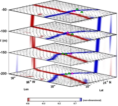
Fig. 2. FTLEs computed from 10 day trajectories and scaled by the
maximum value within each layer, stagnations points (magenta bul-lets), nearby temperature saddle points (green bulbul-lets), and velocity field for 10 June 2010 at depths 50, 100, 150, and 200 m. The blue and red curves denote the stable and unstable ridges of the FTLEs, respectively, derived from forwards, respectively backwards, in time computations.
and are often not well resolved in general circulation models. In the case at hand, vertical velocities can at best be derived from the continuity equation, which relies on noisy derivative estimates. Consequently, we rely here on the 2×2 submatrix
F= ∂x
∂x0
=
"∂x
∂x0
∂x
∂y0
∂y
∂x0
∂y
∂y0
#
, (3)
neglecting vertical motion, as is commonly done. Sulman et al. (2013) provides justification that the manifold location is adequately captured with this approximation.
In the computations presented here, an explicit, adaptive-step, fourth order Runge–Kutta scheme is used to solve the system of ordinary differential equations:
dx
dt =v, t∈ [t0, t0+1t], (4)
with trilinear interpolation in space and time of the model velocitiesv. All derivatives are estimated using second-order centered differencing. The singular values of F are deter-mined using the known analytic expression for 2×2 matrices.
4 FTLEs as surrogates for attracting and repelling manifolds
A cube plot of FTLEs calculated over 10 days in both for-ward and backfor-ward time is shown in Fig. 2. Forfor-ward-time FTLEs are shown in red, those in backward-time in blue. The ridges are easily discerned in these fields. Note that for plot-ting purposes, the FTLE field in each layer has been scaled
by the maximum value achieved in that layer within the re-gion of interest. Clearly, this does not affect the ridge loca-tion. The forward-time ridges near the intersection are the “stable” LCS, as they approximate the unstable manifold. Similarly, the backward-time ridges near the intersection are the “unstable” LCS, as they approximate the stable manifold. To simplify the language, we will refer to these as “unstable and stable FTLE ridges”. Strong FTLE ridges with a per-sistent intersection are generally good surrogates for these manifolds, with the critical trajectory coinciding with the in-tersection (Peacock and Dabiri, 2010; Branicki and Wiggins, 2010).
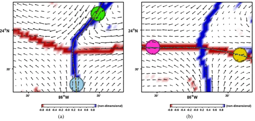
Before analyzing the relationship between the FTLE, ve-locity, and temperature fields (see Sect. 5), we consider the issue whether the FTLE ridges associated with the LCS separation truly depict the attracting and repelling mate-rial surfaces. The strategy to show this is to evolve circu-lar fluid blobs that straddle the stable and unstable ridges. On 5 June 2010 two blobs were initialized along the stable (blue) ridge at 50 m near the edge of the domain as shown in panel (a) in Fig. 3. By 10 June 2010, these blobs develop into thin curves lying along the unstable (red) ridge, as shown in panel (b). Similarly, the two circular blobs shown in panel (b) straddling the unstable (red) ridge were evolved backwards for 5 days, at which time, as seen in panel (a), they align along the middle of the stable (blue) ridge. Figures 4 through 6 show the results of similar calculations at 100, 150, and 200 m.
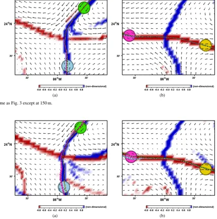
At the three shallower depths, shown in Figs. 3–5, the ad-vected blobs collapse to lines that fall on top of each other along the appropriate FTLE ridge. A minor exception occurs at 150 m, where a small separation between the two curves can be seen at the southern edge on 5 June 2010 and on the western edge on 10 June 2010. At 200 m, on the other hand, two of the four blobs continue to exhibit non-zero area at the end of the integration. The alignment with each other and with the FTLEs is also degraded. This discrepancy seems large by comparison with results at the other levels, but in fact the curves deviate at most by about 3 km, a level of agreement we originally anticipated at all depths.
(a) (b)
Fig. 3. Ridges in the scaled FTLE field at depth 50 m for (a) 5 June 2010 and (b) 10 June 2010. The green and aqua circles in panel (a) depict
the fluid blobs that were advected forwards 5 days and shown in the curve lying in the unstable (red) FTLE ridge on 10 June 2010. Similarly the magenta and yellow circles in panel (b) were advected backwards 5 days and shown in the curves lying in the stable (blue) FTLE ridge on 5 June 2010.
(a) (b)
Fig. 4. Same as Fig. 3 except at 100 m.
5 Connecting hyperbolicity in the temperature and flow fields
Now that we have established that the FTLEs are excellent surrogates for transport barriers in this region, attention is turned to the relationship between the LCS and the structure of the temperature field as it varies with depth. As noted ear-lier, no such description exists in the literature.
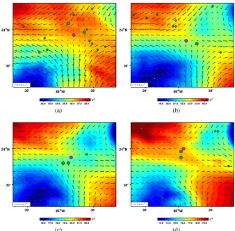
Figure 7 shows the temperature field at 50, 100, 150, and 200 m for the boxed region shown in Fig. 1 along with the velocity field at these depths on 10 June 2010. Also shown
(a) (b)
Fig. 5. Same as Fig. 3 except at 150 m.
(a) (b)
Fig. 6. Same as Fig. 3 except at 200 m.
computed using second-order centered differencing. Saddle points within 20 km of the stagnation point are plotted with larger symbols. The saddle structure of the temperature field is clearly evident at all depths, even though small-scale varia-tions in the field generate many additional local saddle points in the upper layers. Along the northwest–southeast axis the temperature reaches a minimum near 85.6◦W, 23.8◦N.
Along the northeast–southwest axis this same region is a maximum. As seen in the figure, the stagnation points are lo-cated near saddle points, and their geographic location varies little with depth.
The FTLE cube plot in Fig. 2 also depicts the veloc-ity field, the stagnation points, and those saddle points within 20 km of the stagnation points. In agreement with
the theoretical analysis of Haller and Poje (1998) for slowly varying flows, all three occur within a few kilometers of each other. Moreover, all three are nearly vertical within the depth region analyzed here. As evident from the colored streaks on the vertical planes in the figure, both LCS drop nearly verti-cally through the water column as well.
The analysis was repeated for 5 June 2010 with similar re-sults (not shown). The critical points are roughly 25 km to the southwest at approximately 85.9◦W, 23.7◦N, but the
(a) (b)
(c) (d)
Fig. 7. Plots of the contours and saddle points (green bullets) of the temperature field, together with the velocity field and the stagnation points
(magenta bullets) for 10 June 2010 at depths (a) 50, (b) 100, (c) 150, and (d) 200 m. Saddle points further than 20 km from the stagnation points are marked with smaller symbols and do not appear in Fig. 2.
6 Summary and discussion
The FTLEs revealed a resilient intersection of the stable and unstable ridges in the vicinity of 86◦W, 23.8◦N. We were able to track this feature at 50 m from 13 May to 15 June 2010 by daily maps of the FTLE field (not shown), a period of 34 days. The analysis here focuses on the period 5–10 June 2010, a period when Eddy Franklin was observed to pinch off from the Loop Current.
Our analysis of the model temperature and velocity fields showed that during the period of interest stagnation and tem-perature saddle points were found within 4 to 8 km of the FTLE ridge intersection. Moreover, all these features were tracked in a nearly vertical line from the surface to 200 m over the 5 day period. This gives an incontrovertible answer to the first two questions posed in the Introduction: one, the LCS as derived from the FTLE fields are nearly vertical sur-faces. This structure does not change significantly over the 5 day interval studied, but rather is translated and rotated as a whole by the flow. Two, at every level the FTLE ridge in-tersection and the saddle points of the temperature field were
within two grid cells of each other. The close proximity in-dicates that for mesoscale features, such as the one studied here, mere observations of the temperature field can locate the hyperbolic critical point of the velocity field.
To show that the FTLE ridges are indeed surrogates for the attracting and repelling manifolds, we evolved circular blobs of fluid, initialized along the stable ridges on 5 June 2010, for 5 days and found that they lay along the unstable ridges on 10 June 2010. When blobs were initialized along the unstable FTLE ridges on 10 June 2010 and then advected backwards in time, they coincided with the stable ridges on 5 June 2010. In the vicinity of the intersection of FTLE ridges there is now convincing evidence that these are indeed excellent surro-gates for distinguished manifolds. However, the slight devi-ation of the FTLEs from the advected blobs at 200 m shows this is not always the case and that care must be taken when interpreting FTLE ridges as manifold surrogates.
200 m of the water column. This, however, is not consistent with the generally accepted view that the density structure of mesoscale eddies is lens shaped. Consequently, Branicki and Kirwan (2010) speculated that vertical structure of the transport barriers could be attributed to an artifact of their general circulation model. However, three different studies using three different general circulation models with varying resolutions studying two quite different parts of the world’s oceans have now reported essentially the same vertical struc-ture for transport barriers. It would seem then that this is a common characteristic of mesoscale transport barriers and not model artifacts. We emphasize that the vertical structure is not likely to be a universal feature, however. Multipole cir-culations spanning the mixed layer, with smaller deformation radii, and under the influence of topographic features most likely will exhibit pronounced vertical skewing of material transport surfaces.
The close proximity of the stagnation points and the FTLE ridge intersections, although satisfying, is not unexpected. Haller and Poje (1998) showed that in slowly evolving flows, if there is a stagnation point, there should be a distinguished hyperbolic trajectory nearby. As noted in the Introduction, for steady flows these points coincide. Their analysis was purely kinematic and thus did not provide any criteria on how close these features might be. Toner et al. (2003) used the neighborhood trait of distinguished hyperbolic trajecto-ries and stagnation points to find material lines governing the evolution of chlorophyll patterns in the eastern Gulf of Mexico. Thus, there is prior observational confirmation of the close proximity of these features. For the feature studied here this distance is at most 8 km.
The nearness of the temperature field saddle point to the FTLE ridge intersection and stagnation point has dynamical implications. First, the fact that there is some displacement from the intersection is indicative of non-stationarity in the flow. Using the temperature as a surrogate for the geopoten-tial, the proximity of the saddle points in this field with the stagnation points in the velocity field demonstrates answers to the third question posed in the Introduction: geostrophy is the dominant dynamical balance in this region. Since the velocities are quite small near the intersection yet increase substantially outwards, and the velocity gradients are close to the local value of the Coriolis parameter in magnitude a near-geostrophic balance was not apparent at the outset. In fact, we do not anticipate such near-geostrophic balance to hold more generally away from the pinch-off region.
It is noteworthy that over the 5 day period of this study the saddle region comprising the intersections of stable and un-stable FTLE ridges, the stagnation point, and the temperature saddle point remained essentially vertical as it was advected 25 km. This can be deduced from Figs. 3–6. Such persis-tence of vertical structure was surprising since the flow here is strongly hyperbolic with exponential stretching of fluid el-ements.
The FTLE ridges extend out for over 100 km on either side of the intersection, and the FTLE values along the ridges may vary. However, away from the stable–unstable intersections, FTLE ridges become porous and are not necessarily reliable indicators of material transport barriers. Moreover, since the flow is time-dependent, the extent of impermeability is deter-mined by processes remote from the small region analyzed here. Until these issues are satisfactorily resolved, the pre-cise role this saddle region plays in the formation of LCRs is unknown.
Acknowledgements. Support for this research came from the
Office of Naval Research through grants N00014-10-1-0522 and N00014-11-10081 to the University of Delaware, the Office of Naval Research MURIOCEAN 3D+1 grant N00014-11-1-0087, a grant from BP/The Gulf of Mexico Research Initiative, and the Mary A. S. Lighthipe endowment to the University of Delaware. The ICMAT Severo Ochoa project SEV-2011-0087 provided support for publication of this research. The authors wish to thank two anonymous reviewers for their helpful comments.
Edited by: A. Turiel
Reviewed by: two anonymous referees
References
Andrade-Canto, F., Sheinbaum, J., and Zavala Sansón, L.: A La-grangian approach to the Loop Current eddy separation, Nonlin. Processes Geophys., 20, 85–96, doi:10.5194/npg-20-85-2013, 2013.
Bettencourt, J. H., López, C., and Hernández-García, E.: Oceanic three-dimensional Lagrangian coherent structures: A study of a mesoscale eddy in the Benguela upwelling region, Ocean Model., 51, 73–83, doi:10.1016/j.ocemod.2012.04.004, 2012. Bleck, R.: An oceanic general circulation model framed in
hy-brid isopycnic-Cartesian coordinates, Ocean Model., 4, 55–88, doi:10.1016/S1463-5003(01)00012-9, 2002.
Boffetta, G., Lacorata, G., Radaelli, G., and Vulpiani, A.: Detecting barriers to transport: a review of different techniques, Physica D, 159, 58–70, doi:10.1016/S0167-2789(01)00330-X, 2001. Branicki, M. and Kirwan, Jr, A. D.: Stirring: The Eckart
paradigm revisited, Int. J. Eng. Sci., 48, 1027–1042, doi:10.1016/j.ijengsci.2010.08.003, 2010.
Branicki, M. and Wiggins, S.: Finite-time Lagrangian transport analysis: stable and unstable manifolds of hyperbolic trajecto-ries and finite-time Lyapunov exponents, Nonlin. Processes Geo-phys., 17, 1–36, doi:10.5194/npg-17-1-2010, 2010.
Chassignet, E. P., Hurlburt, H. E., Smedstad, O. M., Halli-well, G. R., Hogan, P. J., Wallcraft, A. J., Baraille, R., and Bleck, R.: The HYCOM (HYbrid Coordinate Ocean Model) data assimilative system, J. Marine Syst., 65, 60–83, doi:10.1016/j.jmarsys.2005.09.016, 2007.
Cummings, J. A.: Operational multivariate ocean data assimilation, Q. J. Roy. Meteor. Soc., 131, 3583–3604, doi:10.1256/qj.05.105, 2005.
d’Ovidio, F., Fernández, V., Hernández-García, E., and López, C.: Mixing structures in the Mediterranean Sea from finite-size Lyapunov exponents, Geophys. Res. Lett., 31, L17203, doi:10.1029/2004GL020328, 2004.
Forristall, G. Z., Schaudt, K. J., and Cooper, C. K.: Evolution and Kinematics of a Loop Current Eddy in the Gulf of Mex-ico During 1985, J. Geophys. Res.-Oceans, 97, 2173–2184, doi:10.1029/91JC02905, 1992.
Glenn, S. M. and Ebbesmeyer, C. C.: Drifting Buoy Observations of a Loop Current Anticyclonic Eddy, J. Geophys. Res.-Oceans, 98, 20105–20119, doi:10.1029/93JC02078, 1993.
Haller, G.: Distinguished material surfaces and coherent struc-tures in three-dimensional fluid flows, Physica D, 149, 248–277, doi:10.1016/S0167-2789(00)00199-8, 2001.
Haller, G. and Beron-Vera, F. J.: Geodesic theory of transport bar-riers in two-dimensional flows, Physica D, 241, 1680–1702, doi:10.1016/j.physd.2012.06.012, 2012.
Haller, G. and Poje, A. C.: Finite time transport in aperiodic flows, Physica D, 119, 352–380, doi:10.1016/S0167-2789(98)00091-8, 1998.
Hamilton, P., Donohue, K. A., Leben, R. R., Lugo-Fernandez, A., and Green, R. E.: Loop Current Observations During Spring and Summer of 2010: Description and Historical Per-spective, in: Monitoring and Modeling the Deepwater Hori-zon Oil Spill: A Record-Breaking Enterprise, edited by: Liu, Y., MacFadyen, A., Ji, Z.-G., and Weisberg, R. H., vol. 195 of Geophys. Monogr. Ser., 117–130, AGU, Washington, DC, doi:10.1029/2011GM001116, 2011.
Hurlburt, H. E. and Thompson, J. D.: A Numerical Study of Loop Current Intrusions and Eddy Shedding, J. Phys. Oceanogr., 10, 1611–1651, doi:10.1175/1520-0485(1980)010<1611:ANSOLC>2.0.CO;2, 1980.
Indest, A. W., Kirwan, Jr., A. D., Lewis, J. K., and Reiners-man, P.: A Synopsis of Mesoscale Eddies in the Gulf of Mex-ico, in: Mesoscale/Synoptic Coherent structures in Geophysi-cal Turbulence, edited by: Nihoul, J. C. J. and Jamart, B. M., vol. 50 of Elsevier Oceanography Series, 485–500, Elsevier, doi:10.1016/S0422-9894(08)70203-4, 1989.
Joseph, B. and Legras, B.: Relation between Kinematic Boundaries, Stirring, and Barriers for the Antarctic Polar Vortex, J. Atmos. Sci., 59, 1198–1212, doi:10.1175/1520-0469(2002)059<1198:RBKBSA>2.0.CO;2, 2002.
Kantha, L. H.: Development, testing and implementation of a real-time nowcast/forecast capability for the Gulf of Mexico, Kaiyo Monthly (Japan), 37, 239–256, 2005.
Kirwan, Jr., A. D.: Dynamics of “critical” trajectories, Prog. Oceanogr., 70, 448–465, doi:10.1016/j.pocean.2005.07.002, 2006.
Lapeyre, G.: Characterization of finite-time Lyapunov exponents and vectors in two-dimensional turbulence, Chaos, 12, 688–698, doi:10.1063/1.1499395, 2002.
Large, W. G., McWilliams, J. C., and Doney, S. C.: Oceanic vertical mixing: A review and a model with a nonlocal boundary layer parameterization, Rev. Geophys., 32, 363–403, doi:10.1029/94RG01872, 1994.
Lewis, J. K., Kirwan, Jr, A. D., and Forristall, G. Z.: Evo-lution of a Warm-Core Ring in the Gulf of Mexico: La-grangian Observations, J. Geophys. Res., 94, 8163–8178, doi:10.1029/JC094iC06p08163, 1989.
Liu, Y., Weisberg, R. H., Hu, C., Kovach, C., and Riethmüller, R.: Evolution of the Loop Current System During the Deep-water Horizon Oil Spill Event as Observed With Drifters and Satellites, in: Monitoring and Modeling the Deepwater Hori-zon Oil Spill: A Record-Breaking Enterprise, edited by: Liu, Y., MacFadyen, A., Ji, Z.-G., and Weisberg, R. H., vol. 195 of Geophys. Monogr. Ser., 91–101, AGU, Washington, DC, doi:10.1029/2011GM001127, 2011.
Mendoza, C. and Mancho, A. M.: Hidden Geome-try of Ocean Flows, Phys. Rev. Lett., 105, 038501, doi:10.1103/PhysRevLett.105.038501, 2010.
Mezi´c, I., Loire, S., Fonoberov, V. A., and Hogan, P.: A New Mixing Diagnostic and Gulf Oil Spill Movement, Science, 330, 486–489, doi:10.1126/science.1194607, 2010.
Oey, L.-Y., Ezer, T., and Lee, H.-C.: Loop current, rings and re-lated circulation in the Gulf of Mexico: A review of numerical models and future challenges, in: Circulation in the Gulf of Mex-ico: Observations and Models, edited by: Sturges, W. and Lugo-Fernandez, A., vol. 161 of Geophys. Monogr. Ser., 31–56, AGU, Washington, DC, doi:10.1029/161GM04, 2005.
Peacock, T. and Dabiri, J.: Introduction to Focus Issue: Lagrangian Coherent Structures, Chaos, 20, 017501, doi:10.1063/1.3278173, 2010.
Pierrehumbert, R. T.: Large-scale horizontal mixing in planetary atmospheres, Phys. Fluids A, 3, 1250–1260, doi:10.1063/1.858053, 1991.
Prasad, T. G. and Hogan, P. J.: Upper?ocean response to Hurri-cane Ivan in a 1/25◦nested Gulf of Mexico HYCOM, J. Geophys. Res., 112, C04013, doi:10.1029/2006JC003695, 2007.
Rosmond, T. E.: The Design and Testing of the Navy Operational Global Atmospheric Prediction System, Weather Forecast., 7, 262–272, doi:10.1175/1520-0434(1992)007<0262:TDATOT>2.0.CO;2, 1992.
Rypina, I. I., Scott, S. E., Pratt, L. J., and Brown, M. G.: Investi-gating the connection between complexity of isolated trajectories and Lagrangian coherent structures, Nonlin. Processes Geophys., 18, 977–987, doi:10.5194/npg-18-977-2011, 2011.
Schmitz, Jr., W. J.: Cyclones and westward propagation in the shedding of anticyclonic rings from the loop current, in: Cir-culation in the Gulf of Mexico: Observations and Models, edited by: Sturges, W. and Lugo-Fernandez, A., vol. 161 of Geophys. Monogr. Ser., 241–261, AGU, Washington, DC, doi:10.1029/161GM18, 2005.
Schmitz, Jr., W. J., Biggs, D. C., Lugo-Fernandez, A., Oey, L.-Y., and Sturges, W.: A Synopsis of the Circulation in the Gulf of Mexico and on its Continental Margins, in: Circulation in the Gulf of Mexico: Observations and Models, edited by: Sturges, W. and Lugo-Fernandez, A., vol. 161 of Geophys. Monogr. Ser., 11–29, AGU, Washington, DC, doi:10.1029/161GM03, 2005. Sturges, W., Evans, J. C., Welsh, S., and Holland, W.:
Separation of Warm-Core Rings in the Gulf of Mex-ico, J. Phys. Oceanogr., 23, 250–268, doi:10.1175/1520-0485(1993)023<0250:SOWCRI>2.0.CO;2, 1993.
of Mexico: Observations and Models, edited by Sturges, W. and Lugo-Fernandez, A., vol. 161 of Geophys. Monogr. Ser., 1–10, AGU, Washington, DC, doi:10.1029/161GM02, 2005.
Sulman, M. H. M., Huntley, H. S., Lipphardt, Jr., B. L., and Kirwad, Jr., A. D.: Leaving Flatland: Diagnostics for Lagrangian coher-ent structures in three-dimensional flows, Physica D, 258, 77–92, doi:10.1016/j.physd.2013.05.005, 2013.
Toner, M., Kirwan, Jr., A. D., Poje, A. C., Kantha, L. H., Müller-Karger, F. E., and Jones, C. K. R. T.: Chlorophyll dispersal by eddy-eddy interactions in the Gulf of Mexico, J. Geophys. Res., 108, 3105, doi:10.1029/2002JC001499, 2003.