Entropy production of soil hydrological processes and its maximisation

(1)

Earth Syst. Dynam., 2, 179–190, 2011 www.earth-syst-dynam.net/2/179/2011/ doi:10.5194/esd-2-179-2011

Earth System

Dynamics

Entropy production of soil hydrological processes and its

maximisation

P. Porada, A. Kleidon, and S. J. Schymanski

Max Planck Institute for Biogeochemistry, P.O. Box 10 01 64, 07701 Jena, Germany Received: 17 December 2010 – Published in Earth Syst. Dynam. Discuss.: 28 January 2011 Revised: 13 July 2011 – Accepted: 14 August 2011 – Published: 2 September 2011

Abstract. Hydrological processes are irreversible and

pro-duce entropy. Hence, the framework of non-equilibrium ther-modynamics is used here to describe them mathematically. This means flows of water are written as functions of gra-dients in the gravitational and chemical potential of water between two parts of the hydrological system. Such a frame-work facilitates a consistent thermodynamic representation of the hydrological processes in the model. Furthermore, it allows for the calculation of the entropy production associ-ated with a flow of water, which is proportional to the product of gradient and flow. Thus, an entropy budget of the hydro-logical cycle at the land surface is quantified, illustrating the contribution of different processes to the overall entropy pro-duction. Moreover, the proposed Principle of Maximum En-tropy Production (MEP) can be applied to the model. This means, unknown parameters can be determined by setting them to values which lead to a maximisation of the entropy production in the model. The model used in this study is parametrised according to MEP and evaluated by means of several observational datasets describing terrestrial fluxes of water and carbon. The model reproduces the data with good accuracy which is a promising result with regard to the appli-cation of MEP to hydrological processes at the land surface.

1 Introduction

The analysis and modelling of soil hydrological processes on a global scale is a challenging task, mostly due to in-teractions of the mechanisms involved combined with spa-tial heterogeneity at many scales. Although single processes (e.g. infiltration or bare soil evaporation) are well understood, a unifying quantitative framework to describe hydrological

Correspondence to: P. Porada ([email protected])

behaviour at catchment or larger scales is still missing (Siva-palan, 2005). It is therefore in general not possible to make correct predictions about a certain catchment or region based on a model that has been designed for another catchment. This paper presents an alternative approach to model hy-drological processes. Instead of describing each single pro-cess by a standard empirical theory, the framework of non-equilibrium thermodynamics is used. Thermodynamic meth-ods have already been used by Edlefsen and Anderson (1943) to characterise soil moisture relations and they are the theo-retical basis of common hydrological state variables, such as the matric potential of soil water. Gradients in matric po-tential between two locations can then be used to quantify the tendency of the water to move from high to low poten-tials, e.g. from wet to dry soil. Later, Leopold and Lang-bein (1962) introduced the concept of entropy production into soil hydrology, using the analogy of a thermodynamic heat engine. Similar to heat moving along a temperature gra-dient towards the cooler temperature, the authors formulated runoff as a function of the gradient in the gravitational po-tential of water, which results from topography. By flowing downhill, the water moves from high to low gravitational po-tential, thereby converting potential energy of water into ki-netic energy which is then dissipated into heat by friction. The entropy production of runoff is then proportional to the product of the flow of water and the gradient in gravitational potential. It corresponds to the amount of heat generated by the flow divided by temperature.

(2)

180 P. Porada et al.: Entropy production in soil hydrology system. All exchange flows of water can then be formulated

as functions of gradients in the combined chemical and grav-itational potential of water. In the following, these combined potentials will be denoted by the term “water potential” and they will be expressed by the symbol for chemical poten-tial (µ, e.g. Eq. 1). The implementation of the thermody-namic framework described above into a simple land surface-vegetation model is one main motivation for this paper.

Having formulated flows of water as functions of gradi-ents in water potential, it is straightforward to quantify an entropy budget of the most important soil hydrological pro-cesses. This can be used to illustrate the relative contribu-tions of different processes to the overall dissipation at the land surface.

Another advantage of a thermodynamic formulation of hy-drological processes is the possibility to apply the principle of Maximum Entropy Production (MEP) to the respective models (Kleidon and Schymanski, 2008). This is explained using the example of root water uptake at the global scale. The flow of water from soil to roots is formulated as a linear function of the gradient between soil and root water poten-tial, with a proportionality constantc. The value ofc com-prises all factors affecting the speed of water movement at the root-soil interface such as soil type, macropore density, root density, hydraulic conductivity, etc. which are highly variable at the global scale. In theory, the value ofc at a certain place at a certain time is then determined by all these measurable soil and vegetation properties. However, the re-lation between these properties andcis so unpredictable at the spatio-temporal scale of our model, thatcis characterised by a very large range of values. This is also the reason to as-sume a linear relation between the flow and the gradient in water potential, since it is the simplest model possible, given that not much is known about howc is related to soil and vegetation properties at the scale of this model. At steady state, a maximum in the entropy production associated with root water uptake then results from a trade-off between the flow and the gradient which is driving it: in the presence of alternative pathways (e.g. runoff or bare soil evaporation), high values ofclead to a strong dissipation of the gradient and consequently to a large flow at a small gradient (Schy-manski et al., 2009). Conversely, small values ofclead to a large gradient but a small flow. Since the entropy production is proportional to the product of gradient and flow, it shows a maximum at intermediate values ofc. MEP predicts that the value ofcwhich leads to maximum entropy production is the most probable one, given the model structure and forc-ing. For reviews about MEP see Martyushev and Seleznev (2006); Ozawa et al. (2003).

MEP and other approaches dealing with the dissipation of free energy have been recently used in hydrology and ecol-ogy to predict various properties of land surface systems, ranging from the spatial distribution of biomass in semiarid regions (Schymanski et al., 2010) to preferential flow on hill-slopes (Zehe et al., 2010). The aim of the present paper is to

determine parameter values of a global land surface model (JESSY/SIMBA, Porada et al., 2010) by MEP. In a second step, the model output based on these parameter values is compared with empirical data to test whether the MEP-based prediction leads to realistic results.

This paper is structured as follows: Sect. 2 contains a de-scription of the most important parts of the model used in this study, followed by the model setup in Sect. 3. In Sect. 4, the results of this study are presented, including a parametri-sation of the model according to MEP, an entropy budget of the hydrological cycle at the land surface and an evaluation of the model performance. The paper closes with a discus-sion and an outlook.

2 Model description

The model used in this study simulates terrestrial biogeo-chemical processes in a simple way at the global scale. It consists of a soil model called JESSY (JEna Surface SYs-tem model) and a vegetation model, SIMBA (SIMulator of Biospheric Aspects). JESSY and SIMBA use global grid-ded climate data as input to predict fluxes of carbon and wa-ter at the land surface, including evapotranspiration, runoff and Net Primary Productivity (NPP). Furthermore, reservoirs such as soil water, biomass and soil carbon can be quantified. The models use a global rectangular grid with a resolution of 2.8125 degrees (this corresponds to the T42 resolution).

JESSY and SIMBA are designed to run independently, which means that each of the models can be coupled to other models and they do not have to be run together. JESSY, for instance, needs the value of the vegetation water potential to compute root water uptake. This value can be provided by any vegetation model or it could be prescribed as a boundary condition. This increases the applicability of the two models to biogeochemical questions.

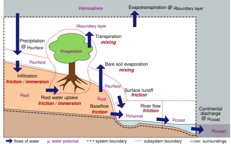
Since the models are described in detail in Porada et al. (2010), only the model parts which have been extended or added for quantifying the entropy production of soil hydro-logical processes are explained here. In JESSY, the entropy production of surface runoff, infiltration, bare soil evapora-tion, root water uptake and baseflow is quantified for each grid cell of the model using the local potentials of water. Soil water storage is represented by a bucket approach. Transpira-tion by the vegetaTranspira-tion and the associated entropy producTranspira-tion is calculated in SIMBA, also for each grid cell. Figure 1 gives an overview of the entropy producing processes considered in the model.

(3)

P. Porada et al.: Entropy production in soil hydrology 181

14 P. Porada et al.: Entropy production in soil hydrology

Infiltration

friction / immersion

Surface runoff

friction

Baseflow

friction µvegetation

µ: water potential

flows of water µ_soil

Root water uptake

friction / immersion

Transpiration

mixing

Bare soil evaporation

mixing

µ_channel

system boundary

River flow

friction µ_surface

subsystem boundary µ_coast

µ_ocean µ_surface

µ_soil

Precipitation @ µsurface

µatmosphere

µboundary layer

surroundings

Continental discharge

@ µ_coast

Evapotranspiration @ µboundary layer

Fig. 22. Overview of the flows of water (black text, regular) and the associated entropy producing dissipative processes (red text, italics) quantified in JESSY and SIMBA. The grey shaded areas correspond to the surroundings of the system.

Fig. 1. Overview of the flows of water (black text, regular) and the associated entropy producing dissipative processes (red text, italics) quantified in JESSY and SIMBA. The grey shaded areas correspond to the surroundings of the system.

between the atmosphere and the surface water reservoirs (rivers, lakes) was not considered since the model does not contain an explicit formulation of the river network. Hy-draulic redistribution cannot be properly described with the simple bucket model used here and is therefore not included. Water flow from the river channel back to the soil does not seem to play a large role at the scale of a model grid cell and is neglected.

Note that all entropy production terms considered in the model are due to processes within the system “land surface”. Since the system is assumed to be in steady state, the entropy produced in the soil or the vegetation is completely exported to the surroundings (Kondepudi and Prigogine, 1998, p. 387). Hence, the external entropy exchange flows are not consid-ered explicitly in our calculation. The assumption of steady state also means that the reservoirs of the hydrological cy-cle at the land surface such as the soil water storage do not change if averaged over long time periods (several decades). A list of the most important model variables and param-eters can be found in Table A1. All model parameter val-ues are globally uniform, which is reasonable considering the simplicity of the model. More complex parametrisations of parts of the model such as different soil types, for instance, would represent an increase in complexity not matched by the other parts of the model, e.g. the vegetation model.

Fur-thermore, the model is not very sensitive to the parameter soil type, probably due to its simplicity.

2.1 The potential of water in different parts of the hydrological system

The potential of water vapour in the atmospheric boundary layer is written as (Kleidon and Schymanski, 2008): µboundary layer = Rspec,vapTair ln(8) +g z (1) whereRspec,vap is the specific gas constant of water vapour, Tair is the temperature of the atmospheric boundary layer, 8is the relative humidity of the air, g is the gravitational acceleration andzis the height above mean sea level.

(4)

equilibrium distribution

soil moisture water table

potential matric potential

gravitational potential

µsoil

0 zc

bedrock zs

0

Fig. 23. Left: Equilibrium distribution of soil water inside the bucket,zs andzc correspond to the height of the surface and the

channel, respectively. Right: Soil water potentialµsoilas a function

of height.

Fig. 2. Left: equilibrium distribution of soil water inside the bucket, zsandzccorrespond to the height of the surface and the channel, respectively. Right: soil water potentialµsoilas a function of height.

van-Genuchten soil water retention curve (van Genuchten, 1980; Mualem, 1976). The value of9M(z)is negative and decreases with decreasing saturation degree. This means that the more unsaturated the soil is, the more work has to be performed to extract water from the soil matrix. The matric potential is written as:

9M(z) = − g αvg

₂

soil(z) 2soil,max

− 1

mvg ₋₁

_n1

vg

(3)

2soilis defined as m3extractable water m−3soil. The rela-tion to saturarela-tionSis:S=2soil/2soil,max=(θ−θr)/(θs−θr) where2soil,max is the relative extractable water content at saturation. θ is the volumetric relative water content of the soil in m3water m−3soil,θris the residual relative soil wa-ter content andθs is the relative water content at saturation as defined in van Genuchten (1980). In the model used in this studyθr andθs are set to values corresponding to the soil type sandy loam (Carsel and Parrish, 1988) which can be found in Table A1. mvg,nvg, andαvgare the parameters of the van-Genuchten soil water retention curve and their values correspond to the soil type sandy loam, too. Under saturated conditions,9M(z)is replaced by the hydraulic head (Atkins, 1998).

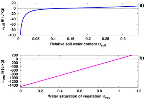
To obtain the value of µsoil for the whole soil column, it is assumed that the water reaches a vertical equilibrium distribution in each time step of the model. Consequently, the soil water potential is constant across the soil profile, µsoil(z)= const. This, however, requires a vertically non-uniform distribution of the water in the soil column (see Fig. 2). Each possible value ofµsoil(z)= const is then as-sociated with a different vertical equilibrium distribution of water. To assign the correct value ofµsoilto a given relative water content of the soil2soil the equilibrium soil moisture distribution whose integral is equal to the value of2soil is calculated. The relationship ofµsoil and water content2soil is shown in Fig. 3.

a)

b)

Fig. 24. a) Soil water potentialµsoilas a function of relative water

content of the soil,Θ_soiland b) vegetation water potentialµvegas a function of the water saturation of the vegetation,Θ_veg.

Fig. 3. (a) Soil water potentialµsoilas a function of relative water

content of the soil,2_soiland (b) vegetation water potentialµvegas a function of the water saturation of the vegetation,2veg.

The height of the soil surface is denoted byzs. The po-tential of free water at the soil surfaceµsurfaceis then set to the gravitational potential atzs since rain is free water. The potential of free water in the river channel,µchannel, is set to the gravitational potential at the heightzcof the channel.

The potential of water in the vegetation,µvegis described by:

µveg = (2veg −1.0) 9PWP (4)

where9PWP is the permanent wilting point which is set to a value of 1471.5 J kg−1_{. This value results from} multiply-ing the wiltmultiply-ing point (150 m, based on Hillel, 1998, p. 144 ff) with the gravitational acceleration. 2veg is the relative wa-ter content of the vegetation (see Fig. 3). µveg decreases linearly with plant available water content (Roderick and Canny, 2005; Schymanski, 2007) to the minimum possible root water potential at the wilting point.

2.2 Calculation of entropy production by flows of water

Root water uptake is described in JESSY as a function of the gradient in water potential between the soil and the vegeta-tion according to:

qroot = croot µsoil −µveg (5) whereµsoilis the soil water potential,µvegis the potential of water in the vegetation andcrootis an effective conductivity at the soil-root interface (see Table A1 and Eqs. 4 and 2). The entropy production of root water uptake is formulated as: σroot = qrootρ

µsoil −µveg Tsoil

(5)

P. Porada et al.: Entropy production in soil hydrology 183 Baseflow is expressed as:

qbase = cbase(µsoil −µchannel) (7) whereµchannel is the potential of water in the river channel andcbasecorresponds to the effective conductivity of the in-terface between the soil and channel. The entropy production of baseflow is calculated as:

σbase = qbaseρ

µsoil −µchannel Tsoil

(8) Bare soil evaporationqevapand transpirationqtransare cal-culated by the minimum of atmospheric demandqepot and the amount of water which is available for evaporation from the soil and the vegetation during a day:

qevap = min

qepot,

2soil1S 1t

(9)

qtrans = min

qepot,

2veg1V

1t

+qroot

(10)

1S and1V are the “bucket depths” of soil and vegetation, respectively, and1t is the model time step which is set to a day. The demandqepotis quantified by an equilibrium evap-oration approach (McNaughton and Jarvis, 1983):

qepot = ds dT ds dT +γ

fnet,0 !

/λ (11)

with ds dT =

epvp1 zT p_vp2+zT

pvp1pvp2pvp3

pvp2 +zT

2 ρ

where zT corresponds to (surface temperature in K – melt-ing temperature of water),fnet,0 is net radiation and _dTds is the slope of the saturation vapour pressure versus tempera-ture relationship. The values of the parametersλ,pvp1,pvp2, pvp3,ρandγ can be found in Table A1. To account for the decrease in hydraulic conductivity at lower soil water con-tents, bare soil evaporation takes place only as long as the difference between the maximum relative soil water content and the actual one is smaller than 0.01. This value is chosen such that, assuming a vertical equilibrium soil water distri-bution, the decrease in hydraulic conductivity at the top of the soil column is approximately 2 orders of magnitude (van Genuchten, 1980). Since bare soil evaporation is small on vegetated surfaces, it is constrained to the fraction of bare soil in each grid cell. The entropy production of bare soil evaporation and transpiration is written as:

σevap =qevapρ

µsoil −µboundary layer Tsurf

(12)

σtrans = qtransρ

µveg −µboundary layer Tsurf

(13)

whereµboundary layer is the water vapour potential of the at-mospheric boundary layer andTsurf is the surface tempera-ture.

Surface runoff is described as saturation excess flow and is consequently controlled by the bucket size (see Table A1). The entropy production of surface runoff is then calculated as:

σsurf =qsurfρ

µsurface −µchannel Tsurf

(14) whereµsurfaceandµchannelare used because free water flows from the soil surface into the nearest river channel. The en-tropy production of the river dischargeqriverinto the oceans, which consists of water from surface runoff and baseflow, is then written as:

σriver = (qsurf+qbase) ρ

µchannel −µmsl

Tsurf

(15) whereµmslcorresponds to the potential of free water at mean sea level, which is set to zero. Since the gradientsµsurface− µchannelandµchannel−µmslare constant, bothσsurfandσriver vary only with the flow rate.

Additionally, entropy is produced during the infiltration of water into the soil, which is formulated as:

σinf = (qrain −qsurf) ρ

µsurface −µsoil Tsoil

(16) where qrain−qsurf is the amount of infiltrated water and µsurface−µsoil is the gradient between free water at the sur-face and bound water in the soil.

3 Model setup

JESSY and SIMBA are run on a global rectangular T42 grid (2.8125 degree resolution) with a climate data set (1971 to 2006; Sheffield et al., 2006) that consists of shortwave ra-diation, downwelling longwave rara-diation, precipitation, av-erage temperature and minimum temperature at 2 m height on a daily basis. Terrestrial longwave radiation and relative humidity are derived from these variables (see Porada et al., 2010 for further information). The model is run until all vari-ables are in a dynamic steady state. The model output is then obtained by averaging over the last 10 yr of the simulation.

3.1 Observational datasets to test the model

JESSY and SIMBA are evaluated by comparing the model output to datasets containing runoff, evapotranspiration, Net Primary Productivity (NPP) and soil carbon. This method has already been used to evaluate the basic version of the model (Porada et al., 2010).

(6)

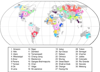
184 P. Porada et al.: Entropy production in soil hydrology to a certain basin. The discharge data is taken from Dai and

Trenberth (2002). An overview of the basins can be found in Fig. A1.

In a second test, modelled evapotranspiration for each grid cell is compared with the one predicted by the empirical Budyko curve (Budyko, 1974). The Budyko-curve estimates evapotranspiration as a function of a climate index, which is calculated from net radiation and precipitation. These are taken from the climate input dataset. The climate index is then calculated for each of the 35 largest river basins as a function of the mean net radiation and precipitation over the basin.

In a third test, the NPP and soil carbon content predicted by SIMBA is compared against global datasets. NPP-data is provided by Cramer et al. (1999) and includes the mean of the NPP-estimates of 17 different vegetation models. In this way, the coupled JESSY/SIMBA model can be compared to other recent global vegetation models. Soil carbon estimates for the first meter of the soil column are taken from IGBP-DIS (1998). The comparison is performed using latitudinal profiles of NPP and soil carbon.

3.2 Determining the MEP-state of root water uptake and baseflow

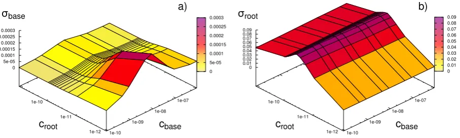
JESSY and SIMBA contain several unknown parameters, which had to be tuned previously (Porada et al., 2010). In this study, two influential parameters,croot andcbase(see Eqs. 6 and 8 and Table A1) are instead determined by MEP. This means they are set to values which lead to a maximisation of the entropy production of the flows they control, namely root water uptake and baseflow. Since all model parameters are global, we maximise the global entropy production of one flow, meaning the sum of all model grid cells, to determine the associated parameter.

Maximising the entropy production of both root water up-take and baseflow requires an iterative approach, since the value of one parameter, e.g.cbase, may affect the MEP-state with respect to the other parameter, e.g.croot, sincecbase de-termines a boundary condition for root water uptake. Hence, a stepwise approach is chosen to find the MEP-states of root water uptake and baseflow: first,cbaseis set to a fixed value and the MEP-state of root water uptake is determined by varyingcroot over several orders of magnitude (see Fig. 4). Then,cbaseis set to another value and another MEP-state of root water uptake is determined. Thus, an MEP-value ofcroot is assigned to each value ofcbase. Finally, the pair of cbase andcrootwhich corresponds to an MEP-state of baseflow is selected (see Fig. 4). This is then used for parametrising the model and evaluating it by comparison with the observational data mentioned in Sect. 3.1.

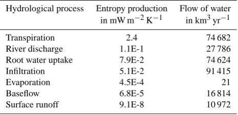
Table 1. Global land surface mean values of entropy production averaged over 10 yr of simulation with the JESSY/SIMBA model which is parametrised according to MEP.

Hydrological process Entropy production Flow of water in mW m−2K−1 in km3yr−1

Transpiration 2.4 74 682

River discharge 1.1E-1 27 786

Root water uptake 7.9E-2 74 624

Infiltration 5.1E-2 91 415

Evaporation 4.5E-4 21

Baseflow 6.8E-5 16 814

Surface runoff 9.1E-8 10 972

4 Results

By varying the two unknown model parameters croot and cbase, the values corresponding to maximum entropy produc-tion of the flows root water uptake and baseflow are deter-mined (see Sect. 3.2). These are croot= 3.5E-11 s m−1 and cbase= 8.6E-9 s m−1(see Fig. 4). The model output obtained by this parametrisation is then evaluated.

4.1 Model evaluation

To evaluate JESSY and SIMBA, the model output is com-pared to observational data described in Sect. 3.1. All vari-ables contained in the datasets are affected by the parameters croot andcbase that are optimised according to MEP. While runoff and evapotranspiration are directly controlled by root water uptake and baseflow, NPP and soil carbon are influ-enced through the effect of root water uptake on the produc-tivity of vegetation. The results of the evaluation are shown in Fig. 5.

The model output shows reasonable agreement with ob-servational data. Both general patterns and absolute val-ues of runoff, evapotranspiration, NPP and soil carbon pre-dicted by the model are close to observations. Considering the Budyko-curve, modelled runoff in the northern temper-ate regions seems to be slightly too high. In comparison with runoff data, however, the model seems to slightly underes-timate runoff in these regions. A possible reason to explain both mismatches is underestimation of precipitation in the model input data of the northern regions, as discussed in Po-rada et al. (2010).

4.2 Entropy budget of soil hydrological processes

The results of the entropy budget of the hydrological cycle (Eqs. 6 to 16) are shown in Fig. 6 and in Table 1. Note the different scale ranges below each plot.

(7)

croot cbase croot cbase

a) b)

σroot

σbase

1e-10 1e-09

1e-08 1e-07

1e-12 1e-11 1e-10 0 5e-05 0.0001 0.00015 0.0002 0.00025 0.0003

0 5e-05 0.0001 0.00015 0.0002 0.00025 0.0003

1e-10 1e-09

1e-08 1e-07

1e-12 1e-11 1e-10 0 0.01 0.02 0.03 0.04 0.05 0.06 0.07 0.08 0.09

0 0.01 0.02 0.03 0.04 0.05 0.06 0.07 0.08 0.09

Fig. 25. Entropy production of (a) baseflow and (b) root water up-take as a function of the two model parameterscbaseandcroot. The

combined MEP-state of baseflow and root water uptake lies at the intersection of the two “ridges” in (a) and (b), the corresponding values can be found in Table A.

Fig. 4. Entropy production of (a) baseflow and (b) root water uptake as a function of the two model parameterscbaseandcroot. The combined

MEP-state of baseflow and root water uptake lies at the intersection of the two “ridges” in (a) and (b), the corresponding values can be found in Table A1.

is the large share of transpiration on the global water bal-ance combined with a strong gradient between vegetation and atmosphere. The latter also leads to a relatively high entropy production of bare soil evaporation compared to the small contribution of evaporation to the water balance (3 or-ders of magnitude smaller than other flows). The gradients associated with root water uptake and infiltration are much smaller, thereby leading to smaller values of the correspond-ing entropy production. While baseflow and surface runoff contribute little to the entropy budget due to the very small gradients in water potential associated with these processes, river discharge results in a relatively high entropy production, especially in mountainous regions characterised by high po-tential energy of water and high runoff.

5 Discussion

Non-equilibrium thermodynamics provides an additional constraint for the formulation of soil hydrological processes, which is usually not considered explicitly. Flows of water are not only constrained by the mass balance, but they are also driven by gradients in water potential between two loca-tions. The formulation of flows and gradients then directly leads to the quantification of the entropy production of hy-drological processes. The entropy production characterises the irreversibility of these processes. This is illustrated in Table 1: although root water uptake is of the same order of magnitude as baseflow, it is much more irreversible due to the strong gradient in water potential between soil and atmo-sphere.

Apart from extending the theoretical basis of a hydrolog-ical model, the thermodynamic approach also makes possi-ble the testing of the Principle of Maximum Entropy Produc-tion (MEP). By applying MEP to the JESSY/SIMBA model, the values of two unknown model parameters that otherwise would have to be tuned can be determined. In spite of the simplicity of the model, the output of the MEP-parametrised

JESSY/SIMBA agrees well with observational data. This suggests that MEP can be used in this case to determine un-known parameter values instead of tuning them. In the scope of behavioral modeling (Schaefli et al., 2011), this means that MEP can be used as an organising principle in soil hydrology at the global scale. The identification of organising principles such as MEP potentially plays a large role for improving hy-drological models, since these principles are assumed to be generally valid and independent of changes in the forcing or in the structure of the system. Using a model as a tool to identify the underlying organising principles thus represents a new approach to modelling hydrological processes and an alternative to parameter tuning.

The reason why deriving model parameter values by MEP leads to realistic predictions is still a matter of discussion. One possible explanation could be that MEP is a physical principle and systems “vary” their properties (expressed by parameters such ascroot andcbase) to achieve maximum en-tropy production. Alternatively, MEP can be interpreted as an algorithm to objectively “guess” some outcomes of a model given the information contained in that model. Hence unknown parameters such ascroot andcbase can be derived since the remaining model structure is sufficient to correctly represent all important processes (Dewar, 2009).

(8)

1e-10 1e-09 1e-08 1e-07

Data from 35 largest river basins [m/s]

Model output from 35 largest river basins [m/s] 0

0.2 0.4 0.6 0.8 1 1.2

0 0.5 1 1.5 2

ET / Epot

P / Epot

a)

b)

c)

d)

P / Epot

E

T

/

E

p

o

t

Model output from 35 largest river basins [m/s]

D

a

ta

f

ro

m

3

5

la

rge

s

t

ri

v

e

r

b

a

sin

s [

m

/s]

N

P

i

n

[

k

g/m²/y

r]

Latitude

S

oil

C

a

rb

o

n

i

n

[

k

g/m

²]

Latitude

Fig. 26. (a) Modelled evapotranspiration averaged over a basin plot-ted against the theoretical Budyko-curve (magenta, dashed) for the 35 world’s largest river basins. (b) Scatterplot of modelled runoff and measured runoff for the 35 largest river basins of the world. •corresponds to humid tropical,humid subtropical,⊡temperate, >_{cold continental and} _×_{(semi) arid climate regions. (c)} Latitu-dinal pattern of modelled NPP (blue, solid) and the mean NPP of 17 global vegetation models (magenta, dashed) latitudinal pattern of modelled (blue, solid) and measured soil carbon (magenta, dashed), both accumulated over the first meter of the soil. All shown model estimates are derived from a MEP-based parametrisation. They are average values over the last 10 years of a simulation.

Fig. 5. (a) Modelled evapotranspiration averaged over a basin plotted against the theoretical Budyko-curve (magenta, dashed) for the 35 world’s largest river basins. (b) Scatterplot of modelled runoff and measured runoff for the 35 largest river basins of the world.• corre-sponds to humid tropical,humid subtropical, temperate,>cold continental and×(semi) arid climate regions. (c) Latitudinal pattern of modelled NPP (blue, solid) and the mean NPP of 17 global vegetation models (magenta, dashed) latitudinal pattern of modelled (blue, solid) and measured soil carbon (magenta, dashed), both accumulated over the first meter of the soil. All shown model estimates are derived from a MEP-based parametrisation. They are average values over the last 10 yr of a simulation.

(see Eq. 11). In the current implementation, this gradient is represented only indirectly by the saturation vapour pressure versus temperature relationship_dTds. Not only flows of water, but also carbon fluxes could be described in thermodynamic terms. MEP could be useful here since the parametrisation of diverse vegetation is difficult and often arbitrary. More-over, additional entropy producing hydrological processes at the land surface could be included in the model. Among these are heat diffusion associated with temperature changes of soil water, irreversible chemical reactions of water with other substances within the soil and physical transformations of the soil, including frost heaving and soil erosion.

(9)

P. Porada et al.: Entropy production in soil hydrology

19

Fig. 27. The global distribution of the entropy production of the

most important soil hydrological processes is shown, quantified by the MEP-based JESSY/SIMBA model: Transpiration, root water uptake, surface runoff, baseflow, river discharge and infiltration. All model estimates are average values over the last 10 years of a sim-ulation.

Fig. 6. The global distribution of the entropy production of the most important soil hydrological processes is shown, quantified by the MEP-based JESSY/SIMBA model: Transpiration, root water uptake, surface runoff, baseflow, river discharge and infiltration. All model estimates are average values over the last 10 yr of a simulation.

production could change on smaller scales. Hence, the con-clusions of this study are restricted to large-scale hydrologi-cal processes. Further errors could arise from the time step of the model: since the potential depends on the water content the gradient is usually reduced by the flow of water during a time step. Hence, the equations that includeµsoil,µveg and µboundary layer may overestimate entropy production by the respective processes since the value of the potential is kept

(10)

188 P. Porada et al.: Entropy production in soil hydrology river discharge are of the same order of magnitude as the ones

calculated by JESSY/SIMBA.

Hence, considering the limitations of the model presented here and the possibilities for future applications, this study can be seen as a first step towards a description of earth system processes which is based on general principles and which is not heavily relying on calibrated parameters.

6 Conclusions

In this study a simple model of water and carbon fluxes at the land surface, JESSY/SIMBA, which contains a ther-modynamic formulation of soil hydrological processes, is used. This framework describes flows of water as functions of gradients in the combined chemical and gravitational

potential of water. It allows for the quantification of an entropy budget of the hydrological cycle at the land surface and also for the testing of the principle of Maximum Entropy Production (MEP). This principle can be used to determine unknown model parameters. Hence, the model is parametrised according to MEP and is then evaluated by comparing the model output with observational data. The results of the evaluation are reasonable which shows that MEP can be successfully applied to the model. Con-sequently, the approach presented here could be used as a basis for further applications of thermodynamics to land surface and vegetation models, leading to increased physical consistency and reliability of these models. This is crucial for understanding and predicting interactions and feedbacks at the land surface resulting from global change.

Appendix A

10 P. Porada et al.: Entropy production in soil hydrology

Appendix B

Overview of river basins.

(11)

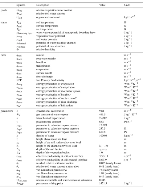
Table A1. Description of model variables and parameters.

Symbol Description Value Units

pools 2veg relative vegetation water content 2soil relative soil water content

Csoil organic carbon in soil kg C m−2

states Tsoil soil temperature K

Tsurf surface temperature K

Tair air temperature K

µboundary layer water vapour potential of atmospheric boundary layer J kg−1

µveg vegetation water potential J kg−1

µsoil soil water potential J kg−1

µchannel potential of water in a river channel J kg−1

µsurface potential of rain at surface J kg−1

8 relative humidity

rates qrain rainfall m s−1

qroot root water uptake m s−1

qbase baseflow m s−1

qtrans transpiration m s−1

qevap evaporation m s−1

qsurf surface runoff m s−1

qriver river discharge m s−1

NPP Net Primary Productivity kg C m−2yr−1

σevap entropy production of evaporation W m−2K−1

σtrans entropy production of transpiration W m−2K−1

σroot entropy production of root water uptake W m−2K−1

σbase entropy production of baseflow W m−2K−1

σsurf entropy production of surface runoff W m−2K−1

σ_river entropy production of river discharge W m−2K−1

σinf entropy production of infiltration W m−2K−1

parameters g gravitational acceleration 9.81 m s−2

RV gas constant of water vapour 461.5 J kg−1K−1

λ latent heat of vaporization 2.45E6 J kg−1

γ psychometric constant 65.0 Pa K−1

pvp1 parameter to calculate vapour pressure 17.269

pvp2 parameter to calculate vapour pressure 237.3 K

pvp3 parameter to calculate vapour pressure 610.8 Pa

ρ density of water 1000.0 kg m−3

z height above mean sea level m

zs height of the soil surface above sea level m

zc height of the channel above sea level zs−1.0 m

1S depth of the soil bucket zs−zc m

1V depth of the vegetation bucket 1.0 m

croot effective conductivity at soil-root interface 3.5E-11 s m−1 cbase effective conductivity at soil-channel interface 8.6E-9 s m−1 θr residual relative soil water content 0.065 (sandy loam)

θs relative soil water content at saturation 0.41 (sandy loam)

αvg van Genuchten parameterα 7.5 (sandy loam)

nvg van Genuchten parametern 1.89 (sandy loam)

mvg van Genuchten parameterm 0.47 (sandy loam)

2soil,max relative extractable soil water content at saturation 0.345

(12)

Acknowledgements. The authors are thankful to Fabian Gans for useful discussions about the topic. We thank the Helmholtz Alliance “Planetary Evolution and Life” for funding and two anonymous reviewers for helpful comments.

Edited by: R. Niven

The service charges for this open access publication have been covered by the Max Planck Society.

References

Atkins, P. W.: Physical Chemistry, 6th Edn., Oxford University Press, Oxford, 1998.

Budyko, M.: Climate and life, Academic Press, New York, 1974. Carsel, R. F. and Parrish, R. S.: Developing Joint Probability

Dis-tributions of Soil Water Retention Characteristics, Water Resour. Res., 24, 755–769, doi:10.1029/WR024i005p00755, 1988. Cramer, W., Kicklighter, D. W., Bondeau, A., Moore III, B.,

Churkina, G., Nemry, B., Ruimy, A., and Schloss, A.: Com-paring global models of terrestrial Net Primary Productiv-ity (NPP): overview and key results, Global Change Biol., 5, 1– 15, doi:10.1046/j.1365-2486.1999.00009.x, 1999.

Dai, A. and Trenberth, K. E.: Estimates of Freshwater Dis-charge from Continents: Latitudinal and Seasonal Vari-ations, J. Hydrometeorol., 3, 660–687, doi:10.1175/1525-7541(2002)003<0660:EOFDFC>2.0.CO;2, 2002.

Dewar, R. C.: Maximum Entropy Production as an Inference Al-gorithm that Translates Physical Assumptions into Macroscopic Predictions: Dont Shoot the Messenger, Entropy, 11, 931–944, doi:10.3390/e11040931, 2009.

Edlefsen, N. E. and Anderson, A. B. C.: Thermodynamics of Soil Moisture, Hilgardia, 15, 31–298, 1943.

Hillel, D.: Environmental Soil Physics, Academic Press, 1998. IGBP-DIS: SoilData(V.0), A program for creating global

soil-property databases, IGBP Global Soils Data Task, France, 1998. Kleidon, A. and Schymanski, S.: Thermodynamics and optimality of the water budget on land: A review, Geophys. Res. Lett., 35, L20404, doi:10.1029/2008GL035393, 2008.

Kleidon, A., Schymanski, S. J., and Stieglitz, M.: Thermodynam-ics, Irreversibility, and Optimality in Land Surface Hydrology, in: Bioclimatology and Natural Hazards, edited by: St˘relcová, K., Mátyás, C., Kleidon, A., Lapin, M., Matejka, F., Bla˘zenec, M., ˘Skvarenina, J., and Holécy, J., Springer, Berlin, Germany, 107–118, doi:10.1007/978-1-4020-8876-6 9, 2009.

Kondepudi, D. and Prigogine, I.: Modern thermodynamics – from heat engines to dissipative structures, Wiley, Chichester, 1998. Leopold, L. B. and Langbein, W. L.: The concept of entropy in

landscape evolution, US Geol. Surv. Prof. Pap., 500-A, 20, 1962. Martyushev, L. M. and Seleznev, V. D.: Maximum entropy produc-tion principle in physics, chemistry and biology, Phys. Rep., 426, 1–45, doi:10.1016/j.physrep.2005.12.001, 2006.

McNaughton, K. G. and Jarvis, P. G.: Predicting effects of vegeta-tion changes on transpiravegeta-tion and evaporavegeta-tion, in: Water Deficits and Plant Growth, edited by: Kozlowski, T. L., Academic Press, New York, 7, 1–47, 1983.

Mualem, Y.: A new model for predicting the hydraulic conductivity of unsaturated porous media, Water Resour. Res., 12, 513–522, doi:10.1029/WR012i003p00513, 1976.

Ozawa, H., Ohmura, A., Lorenz, R. D., and Pujol, T.: The second law of thermodynamics and the global climate system – a review of the maximum entropy production principle, Rev. Geophys., 41, 1018, doi:10.1029/WR012i003p00513, 2003.

Porada, P., Arens, S., Buend´ıa, C., Gans, F., Schymanski, S. J., and Kleidon, A.: A simple global land surface model for bio-geochemical studies, Technical Reports, Max-Planck-Institut f¨ur Biogeochemie, Jena, Germany, 18, 2010.

Roderick, M. L. and Canny, M. J.: A mechanical interpretation of pressure chamber measurements – what does the strength of the squeeze tell us?, Plant Physiol. Biochem., 43, 323–336, doi:10.1016/j.plaphy.2005.02.014, 2005.

Schaefli, B., Harman, C. J., Sivapalan, M., and Schymanski, S. J.: HESS Opinions: Hydrologic predictions in a changing environ-ment: behavioral modeling, Hydrol. Earth Syst. Sci., 15, 635– 646, doi:10.5194/hess-15-635-2011, 2011.

Schymanski, S. J.: Transpiration as the Leak in the Carbon Fac-tory: A Model of Self-Optimising Vegetation, Ph.D. thesis, The University of Western Australia, Perth, Australia, 2007. Schymanski, S. J., Kleidon, A., and Roderick, M. L.:

Eco-hydrological Optimality, in: Encyclopedia of Hydrologi-cal Sciences, edited by: Anderson, M. G. and McDon-nell, J. J., John Wiley & Sons, Ltd, New York, USA, doi:10.1002/0470848944.hsa319, 2009.

Schymanski, S. J., Kleidon, A., Stieglitz, M., and Narula, J.: Maxi-mum Entropy Production allows simple representation of hetero-geneity in arid ecosystems, Philos. T. Roy. Soc. B, 365, 1449– 1455, doi:10.1098/rstb.2009.0309, 2010.

Sheffield, J., Goteti, G., and Wood, E. F.: Development of a 50-yr high-resolution global dataset of meteorological forc-ings for land surface modeling, J. Climate, 19, 3088–3111, doi:10.1175/JCLI3790.1, 2006.

Sivapalan, M.: Pattern, Process and Function: Elements of a Uni-fied Theory of Hydrology at the Catchment Scale, in: En-cyclopedia of Hydrological Sciences, edited by: Anderson, M. G., John Wiley & Sons, Ltd, New York, USA, 193–219, doi:10.1002/0470848944.hsa012, 2005.

van Genuchten, M. T.: A closed-form equation for predicting the hydraulic conductivity of unsaturated soils, Soil Sci. Soc. Am. J., 44, 892–898, 1980.

V¨or¨osmarty, C., Fekete, B., Meybeck, M., and Lammers, R.: Geomorphometric attributes of the global system of rivers at 30-minute spatial resolution, J. Hydrol., 237, 17–39, doi:10.1016/S0022-1694(00)00282-1, 2000.