Open Plot Project: an open-source toolkit for 3-D structural data analysis

(1)

www.solid-earth.net/2/53/2011/ doi:10.5194/se-2-53-2011

Solid Earth

Open Plot Project: an open-source toolkit for 3-D structural

data analysis

S. Tavani, P. Arbues, M. Snidero, N. Carrera, and J. A. Mu ˜noz

Geomodels, Departament de Geodinamica i Geofisica, Facultat de Geologia, Universitat de Barcelona, Barcelona, Spain Received: 12 November 2010 – Published in Solid Earth Discuss.: 6 December 2010

Revised: 28 April 2011 – Accepted: 3 May 2011 – Published: 25 May 2011

Abstract. In this work we present the Open Plot Project, an open-source software for structural data analysis, includ-ing a 3-D environment. The software includes many clas-sical functionalities of structural data analysis tools, like stereoplot, contouring, tensorial regression, scatterplots, his-tograms and transect analysis. In addition, efficient filtering tools are present allowing the selection of data according to their attributes, including spatial distribution and orientation. This first alpha release represents a stand-alone toolkit for structural data analysis.

The presence of a 3-D environment with digitalising tools allows the integration of structural data with informa-tion extracted from georeferenced images to produce struc-turally validated dip domains. This, coupled with many im-port/export facilities, allows easy incorporation of structural analyses in workflows for 3-D geological modelling. Ac-cordingly, Open Plot Project also candidates as a structural add-on for 3-D geological modelling software.

The software (for both Windows and Linux O.S.), the User Manual, a set of example movies (complementary to the User Manual), and the source code are provided as Supplement. We intend the publication of the source code to set the foun-dation for free, public software that, hopefully, the structural geologists’ community will use, modify, and implement. The creation of additional public controls/tools is strongly en-couraged.

1 Introduction

In the last years the rising availability of new technologies and high-quality 3-D seismic data has implied the increasing use of truly 3-D geological models. Due to this,

methodolo-Correspondence to: S. Tavani ([email protected])

gies have been developed to integrate surface and sub-surface geological data to build geologically constrained 3-D models (e.g. Fern´andez et al., 2004; Frank et al., 2007; Calcagno et al., 2008; Suzuki et al., 2008; Carrera et al., 2009; Caumon et al., 2009; Jessel et al., 2010). However, the information used for building 3-D models commonly includes a limited suite of available data, particularly for data collected in the field. The geometries of geological surfaces, like faults and layers, are by far considered the most important data. Methodolo-gies for the construction of geological models rarely incor-porate other information, like the attributes of the deforma-tion pattern, which can be crucial for extrapolating data into the undersampled portions of the aimed model (e.g. Thor-bjornsen and Dunne, 1997; Tavani et al., 2006). Tools for structural data analysis implemented in commonly used 3-D CA3-D-like geological modelling software, like GoCad (by Paradigm), Dmove (by Midland Valley Exploration) or 3-DGeoModeller (by Intrepid Geophysics and BRGM), are neither free nor open-access, and can have limitations in the interactive structural data selection, managing and sub-sequent analysis. This also affects the managing of bedding attitude data. Robust methodologies for 3-D reconstruction based on consistent bedding data interpolation and extrapola-tion require the use of in-house developed tools (e.g. Carrera et al., 2009). In addition, widely used software for struc-tural data analysis does not incorporate 3-D tools (or these are quite basic) and the “communication” between the 3-D modelling software and the structural data analysis tools is frequently neither simple nor direct. Therefore, the whole process of 3-D reconstruction requires frequent and time-consuming passages between different CAD-like tools, soft-ware for structural data analysis, and in-house developed rou-tines (e.g. Fern´andez, 2004).

(2)

modelling and structural data analysis tools, and (2) provid-ing an advanced toolkit for structural data analysis. The software is entirely written in RealBasic 2009r2 (RealSoft-ware Inc, 2009), a multi-platform basic language (running on Linux, Windows and Mac), which includes a 3-D con-trol and represents an optimal compromise between speed, 3-D graphic quality and programming easiness. The last point is particularly important to us, as the main intent of the Open Plot project is to provide an open source code (the code is here provided as Supplement). A set of functionali-ties are provided in this first release. These have, however, the main purpose of inviting the structural geology commu-nity to modify/implement the code, returning it to the com-munity.

2 Summary of software architecture and functionalities

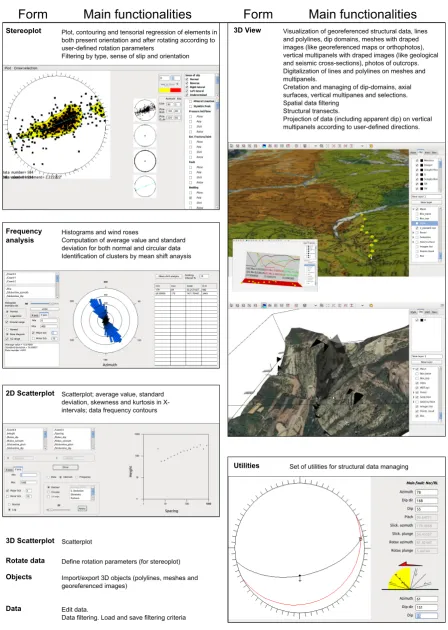
The main functionalities of the software are described in Fig. 1. These include classical tools, like stereoplot, contour-ing, histograms and structural transects, which are present in other non-commercial software for structural data analysis (e.g. GEOrient by Holcomb, 2010; OXSStereonet by Car-dozo and Allmendinger, 2011; Daisy by Salvini, 2011). In addition, a 3-D environment is present in Open Plot Project, allowing the management of georeferenced structural data (like bedding, fault, joints, mineral lineations etc.) and 3-D objects like meshes, polylines, vectors, dip-domains, etc. Many of these 3-D objects can be directly created within the 3-D framework of Open Plot and “structural” attributes are assigned to them.

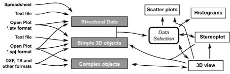
The complete description of functions and procedures for importing, saving, managing and exporting data is illustrated in the User Manual, which is attached to this work. In this section we summarise the internal workflow of the software. The working philosophy of Open Plot project is schemat-ically illustrated in Fig. 2. Three different types of data can be loaded, converted into the Open Plot format (eventually saved) and plotted. Structural data, basic 3-D objects and complex objects:

– Structural data are punctual objects, like bedding sur-faces, mesofaults, mineral lineations, AMS tensor, and include lineations, planes (eventually with slickenlines), and tensors. For these elements, each record can include user-defined attributes. As an example, a joint with as-sociated spacing, orientation, author, date, lithological information, etc., is a structural datum.

– Basic 3-D objects include “simple” 3-D surfaces (i.e. planar polygons and vertical panels/multipanels), polylines, vectors and triangles. The record associated with vectors, triangles, polygons and polylines can in-clude user-defined attributes and, in all the cases, ori-entation data are computed for them. On the contrary, vertical multipanels are purely geometrical objects with

no attributes. These are used to create and save selec-tions, drape images (like seismic sections or geological cross sections), and to project structural data (including apparent dip) along the multipanel trace (i.e. to create structural transects, e.g. Wise and McCroy, 1982; Ta-vani et al., 2006).

– Complex objects include triangular meshes and im-ages. In particular, three types of images can be loaded. (1) Textures: non-georeferenced images, which can be draped on vertical panels. (2) Maps: georeferenced images, which can be draped on meshes. (3) Image lists: arrays of images (typically photos of outcrops). Structural data and basic 3-D objects can be saved in both *.stv and *.spj format. Complex objects can be saved only in *.spj format. The first format is, in a few words, a NxM matrix of strings with an initial header where the number of columns and rows are specified. Such a format allows easy import of a *.stv file in a spreadsheet, modification and re-import in the Open Plot project (with a simple copy and paste procedure). Data editing and modification in external spread-sheets is thus recommended, although a data editing tool is provided within the software. The structure of *.spj files is, in its first part (where structural data and basic 3-D objects are stored), identical to that of *.stv files. In the second part of the file, points and triangles of meshes (if present) are listed, and then, in binary format, all the images.

Structural data and basic 3-D objects can be selected by fil-tering their attributes and then plotted in five windows: Fre-quency analysis, 2-D Scatterplot, 3-D Scatterplot, Stereoplot and 3-D View. In the first three cases, a new matrix including only the selected portion of the dataset is generated. This new matrix is sent to the corresponding plotting window, just for data displaying and analysis, not for editing or modification. In the case of stereoplot, the corresponding temporary matrix is linked to the main one and many operations can be per-formed on the selected portion of the dataset. These include the selection of a new sub-dataset, the assignment of new at-tributes, and the “storage” of directions that can be used in the 3-D View window to create new data. The functionalities of the 3-D View window are much more complex. Structural data, basic 3-D objects and complex objects can be displayed in this window. Similarly to the Stereoplot window, the dis-played objects are linked to the main matrix. Basic 3-D ob-jects can be created/erased here (also with the aid of tools present in the Stereoplot window) and many operations can be performed on the selected dataset. These operations in-clude the projection of data along panels and the selection of sub-dataset, which can be directly sent to the other plotting windows.

(3)

Form

Stereoplot Plot, contouring and tensorial regression of elements in both present orientation and after rotating according to user-defined rotation parameters

Filtering by type, sense of slip and orientation

Histograms and wind roses

Computation of average value and standard deviation for both normal and circular data Identification of clusters by mean shift anaysis Frequency

analysis

Scatterplot; average value, standard deviation, skewness and kurtosis in X-intervals; data frequency contours 2D Scatterplot

Scatterplot 3D Scatterplot

Visualization of georeferenced structural data, lines and polylines, dip domains, meshes with draped images (like georeferenced maps or orthophotos), vertical multipanels with draped images (like geological and seismic cross-sections), photos of outcrops. Digitalization of lines and polylines on meshes and multipanels.

Cretation and managing of dip-domains, axial surfaces, vertical multipanes and selections. Spatial data filtering

Structural transects.

Projection of data (including apparent dip) on vertical multipanels according to user-defined directions. 3D View

Define rotation parameters (for stereoplot) Rotate data

Import/export 3D objects (polylines, meshes and georeferenced images)

Objects

Edit data.

Data filtering. Load and save filtering criteria Data

Set of utilities for structural data managing Utilities

Main functionalities

Form

Main functionalities

(4)

Structural Data

Spreadsheet Text file Open Plot *.stv format

DXF, TS and other formats

Simple 3D objects

Text file Complex objects Open Plot *.spj format Data Selection Histograms Scatter plots Stereoplot 3D view

Fig. 2. Schematic working philosophy of Open Plot.

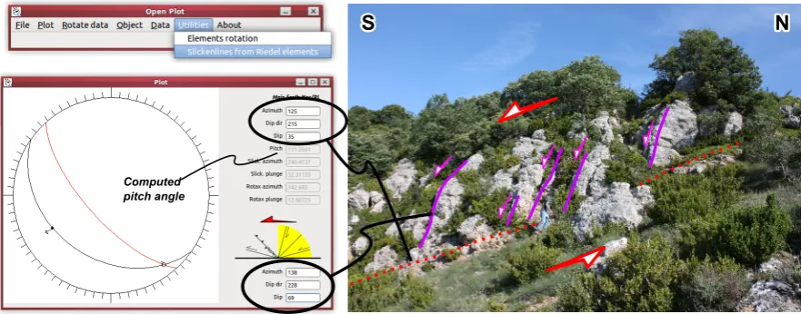
Additional functionalities, which do not require the load-ing of data, are present in Open Plot as, for example, the com-putation of fault slip direction from Riedel structures (Riedel, 1929).

3 Case study

In this section we illustrate the application of Open Plot project to the Poza de la Sal Diapir case study. Two addi-tional short examples are in the Supplement. Firstly, we sum-marise the geological setting of the study structure (for its full description see Quinta et al., 2011) and then we describe the procedures we used for data collection and analysis.

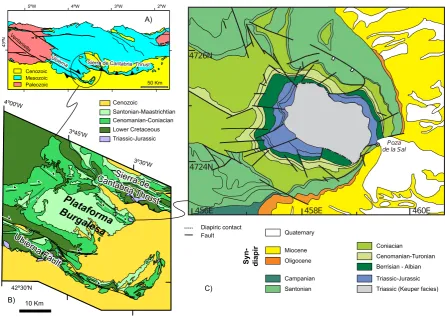
The Poza de la Sal diapir is a slightly elliptical structure lo-cated in the Cantabrian Mountains (Western Pyrenean Belt, Spain) (Fig. 3). This portion of the belt resulted from the Cenozoic inversion of an Upper Jurassic to Lower Creta-ceous basin, which developed during an extensional stage associated with the opening of the of the North Atlantic and Bay of Biscay (Le Pichon and Sibuet, 1971; Garc´ıa-Mond´ejar, 1996; Mu˜noz, 2002). The Poza de la Sal Di-apir is located at the eastern termination of an open anticline striking about WNW-ESE (Fig. 3b). This anticline hosts WNW-ESE striking right-lateral faults (resulting from the reactivation of inherited late-rifting extensional faults) and forms part of the Plataforma Burgalesa domain, which is a slightly folded area where Upper Cretaceous post-rift sed-iments are exposed. The Sierra de Cantabria far-travelled Frontal Thrust and the Ubierna right-lateral Fault System bind the Plataforma Burgalesa domain to the north and to the south, respectively, both of them striking about WNW-ESE in the study area. Oligocene and Miocene growth strata indi-cate the alpine origin of the Poza de la Sal Diapir but, due to the proximity of major structures having different kinemat-ics, two hypotheses exist about the tectonics framework re-sponsible for the development of the study structure. (1) The diapir represents part of the contractive framework and has developed due to the squeezing of Triassic evaporites in the core of the WNW-ESE striking anticline; (2) the diapir be-longs to the right-lateral strike-slip system and has developed at the eastern extensional horsetail termination of the WNW-ESE striking fault system. Field data were integrated with orthophotos interpretation to provide insights about the evo-lution of the diapir.

3.1 Step 1 field data collection

Mesostructural data collected in the field can be directly in-troduced in Open Plot Pj., together with photographs and sketches of outcrops (Fig. 4), or introduced in a spreadsheet and later imported into Open Plot. Both procedures were used in the Poza de la Sal Diapir, where 77 bedding sur-face, 408 joints, 341 faults (69 of them having slickenlines) and 37 fault-related deformation structures (i.e. Riedel’s ele-ments) where measured. Joints were mostly measured in the western portion of the study area while faults were collected in the entire diapir. The Slickenlines from Riedel function were used to compute the slip direction of faults having as-sociated deformation structures but no slickenlines (Fig. 5). Consequently, the number of faults with a pitch angle was increased to 97. The azimuth and dip of the reference bed-ding were collected for each datum, although these are not software-defined fields. This allowed rotation of the bedding to the horizontal and analysis of the pre-tilting orientation (and kinematics) of mesostructural data. The rotation func-tion of Open Plot is mainly designed for this purpose. To restore a dataset to the pre-tilting attitude, the reference bed-ding azimuth must be set as a rotation axis strike, the rotation axis plunge field must be empty, and the reference bedding dip must be set as rotation angle (Fig. 6). It is important to re-mark that reference bedding azimuth must be expressed with the right-hand rule.

3.2 Step 2 data analysis

(5)

20

Poza de la Sal

4724N 4726N

460E

456E 458E

Cenozoic

Santonian-Maastrichtian Cenomanian-Coniacian Lower Cretaceous Triassic-Jurassic

10 Km

Diapiric contact

Fault Quaternary

Miocene Oligocene

Campanian Santonian

Coniacian Cenomanian-Turonian Berrisian - Albian

Triassic-Jurassic Triassic (Keuper facies)

S

yn

-diapir

4º00'W

3º45'W

3º30'W

42º30'N

5ºW 4ºW 3ºW 2ºW

43ºN

50 Km

Sierra de Cantabria Thrust

Ub ierna

Ventan iella

Cenozoic Mesozoic Paleozoic

A)

B)

C) Plataf

orma Bu

rgales a

Ub ierna

Fau_lt

Sierra de Cantab

ria Th_rust

Sierra de Cantabria Thrust

Ub ierna

Fau_lt

Sierra de Cantab

ria Th_rust

Fig. 3. Geological maps. (a) Western Pyrenean Belt. (b) Southern portion of the Cantabrian Mountains. (c) Poza de la Sal Diapir.

Create a new file and define fields Edit the dataset and, eventually, add new records

In the 3D view mouse right-click to add a new datum or a set of images in the selected position

Fig. 4. Procedures to introduce data and photos of outcrops in Open Plot Pj.

In outcrops characterised by steeply dipping beds, prob-lems exist for defining the relative chronology between tilt-ing and the development of many elements. In the followtilt-ing we illustrate, as an example, how we managed normal faults

(6)

S

N

S

N

Computed pitch angle

Fig. 5. How to use the Slickenlines from Riedel elements utility to get the fault pitch angle.

the red colour to normal faults having rotaxes striking WNW-ESE. The stereoplot window was then reloaded (to make ef-fective the colour change) and fault data were analysed in their present orientation. This revealed that, in their present orientation, right-lateral faults having NE-SW striking slick-enlines mostly include “red” elements. Similarly, N-S strik-ing left-lateral faults mostly include “red” elements. This im-plies that NE-SW striking right-lateral faults and N-S strik-ing left-lateral faults probably represent a tilted conjugated normal fault system.

A similar problem affects reverse faults having rotaxes striking about NNW-SSE. These few elements are at a high angle to bedding and are not present in the unrotated anal-ysis (Fig. 8). Following the above-described procedure we recognised that in the unrotated projection, these elements are steeply-dipping normal faults. A consistent interpretation is that NNW-SSE striking normal faults include both pre and post-tilting elements and, accordingly, these could be syn-diapir. NNW-SSE striking joints, which run parallel to the above described extensional fault set, would be syn-diapir too. The same is for WSW-ENE striking normal faults and joints, which are characterised by ambiguous crosscutting relationships with the WSW-ENE striking extensional ele-ments. Accordingly, the working hypothesis is that the diapir has developed within a stress field having a positive near ver-ticalσ1 and two negative components oriented NNW-SSE and WSW-ENE.

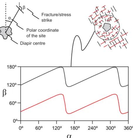
As explained in Quint`a et al., (in press), the interaction be-tween doming-related and regional stress fields is expected to produce variations of the orientation of the local stress field (and accordingly of the strike of syn-diapir elements), which depend on the polar coordinates with respect to the diapir centre (Fig. 10). To evaluate if NNW-SSE and WSW-ENE striking extensional elements were characterised by az-imuthal variations around the diapir, we proceeded as

fol-lows: The dataset was imported in a spreadsheet and the co-ordinate of each element with respect to the diapir centre was computed. Another field was created corresponding to the azimuth computed in the 0–180◦ _{range. This new file was}

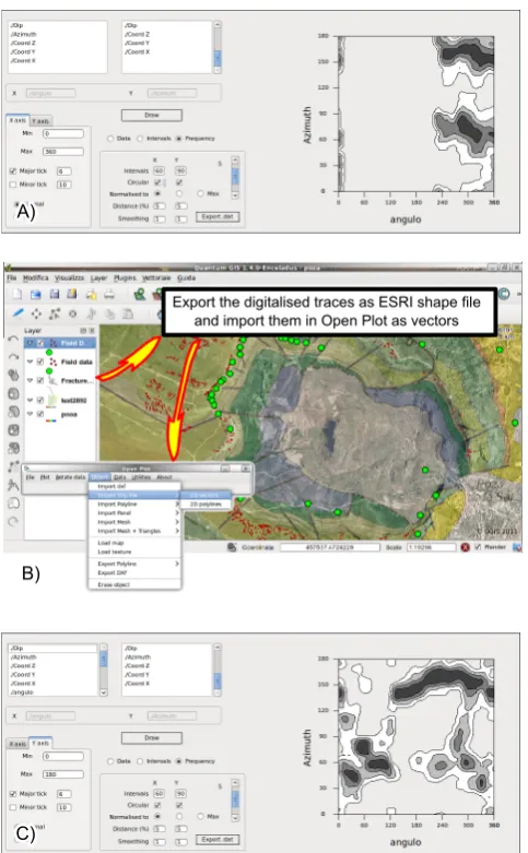
then reimported in Open Plot (using the copy and paste pro-cedure illustrated in the User Manual). As joints are much more abundant than faults (and have been specifically col-lected for this analysis) we analysed joints azimuth around the diapir. In particular, data from the western portion of the diapir were analysed (377 joints data), their position is closely spaced. The few joints collected in the other portions of the diapir were not used, due to their sparse spatial distri-bution. To do this, joints were selected in the data selection window and then in the 2-D scatterplot window their polar angle (X-axis) vs. their azimuth in the 0–180◦range (Y-axis) was plotted (Fig. 11a). Slight but significant variations of the joints’ azimuth were observed at different polar angles. However, the joints were mostly located in the western por-tion of the diapir (due to exposure condipor-tions), which affects the reliability of the result.

(7)

Define rotation parameters

Plot data rotated according to the previously defined parameters

Fig. 6. How to use the rotation function to later project data in their unfolded attitude.

trends of joints (which ensures that most of fracture traces belong to joints) but in a wider range (Fig. 11c). The conclu-sion is that NNW-SSE and WSW-ENE striking joints slightly change their orientation around the diapir, confirming that the regional stress field acting during the diapir growth was char-acterised by sub-horizontal minimum and intermediate stress components striking about WSW-ENE and NNW-SSE. The ambiguous crosscutting relationships and the overall poor quality of the outcrops did not allow a definition of which was the minimum stress component. However, the above-described analysis indicated that the most congruent inter-pretation is that the Poza de la Sal Diapir represents part of the right-lateral strike-slip assemblage. NNW-SSE strik-ing extensional elements would have developed perpendic-ular to a WSW-ENE orientedσ3, kinematically induced by the lateral movement along WNW-ESE oriented right-lateral faults (e.g. Sylvester, 1988). In the extensional horse-tail termination of this right-lateral fault system, an inversion

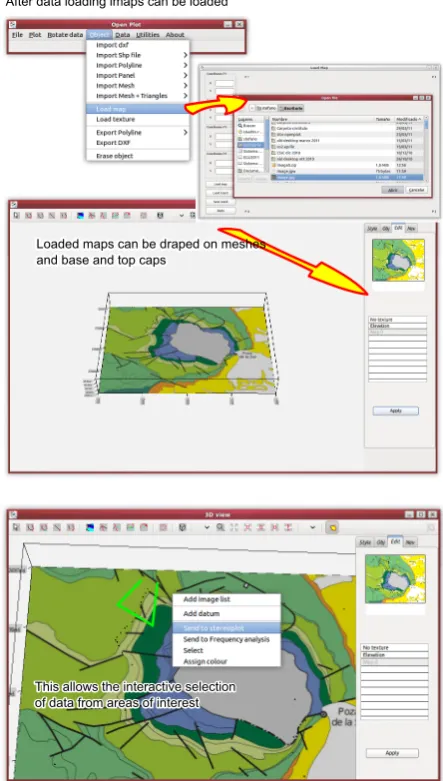
Loaded maps can be draped on meshes and base and top caps

This allows the interactive selection of data from areas of interest This allows the interactive selection of data from areas of interest After data loading lmaps can be loaded

Fig. 7. Procedure for loading maps, draping them on objects in the 3-D view window, and selecting data from an area of interest.

between s2 and s1 occurred, thus s2 oriented NNWSSE. Ac-cordingly, joints striking WSW-ENE have to be regarded as cross-joints (e.g. Gross, 1993) developed perpendicularly to

σ2.

(8)

DN = 408 DN = 408

DN = 23 DN = 27

DN = 12 DN = 21

DN = 33 DN = 20

DN = 10 DN = 10

P ol es t o joi nts R otaxe s no rm al fau lts Ro ta xes reve rse f aul ts S licken line s R.-la te ral fau lts S licken line s L.-la te ral fau lts

C.I. = 3% C.I. = 3%

C.I. = 4.5% C.I. = 3%

C.I. = 3% C.I. = 3%

C.I. = 4% C.I. = 4%

Present orientation After bedding dip removal

Fig. 8. Stereoplots of mesostructural data collected in the Poza de la Sal Diapir. DN and C.I. indicate the data number and the contouring interval, respectively.

data collected in the field and fracture traces easily imported from GIS software. The results obtained in the Poza de La Sal using Open Plot could have been obtained using other software as well. This, however, would have required sev-eral time-consuming passages and, in many cases,

one-by-one data selection in a spreadsheet.

4 System requirements

Open Plot project derives from a basic software developed for work in the field with the first low-cost netbooks. Open Plot project preserves the capability of its ancestor of run-ning on computers with low-cost components (tested down to 900 Mhz Intel Celeron M processor, 512 MB of RAM, In-tel GMA 900 graphic card) and with both Window XP and Ubuntu8.04 or higher OS (it “should” also run on other Linux distributions, provided GTK +2.8 is installed and the window version runs on Linux under Wine). The version for Mac OS is not provided. However,Mac users can easily compile the code. Although the most part of the windows are correctly displayed on 800×480 screens, a minimum screen resolu-tion of 1024×600 is recommended.

5 Concluding remarks

The possibility to easily import different data types from spreadsheets, text files, and other file formats, including meshes and polylines from DXF files, coupled with the sim-ple STV file structure and the presence of a DXF export fa-cility, allow to: (1) easily use Open Plot project as a sort of structural add-on of CAD software, (2) use Open Plot to-gether with other structural tools; (3) use it as a stand-alone toolkit.

In the first case, Open Plot project represents an external add-on allowing import from different sources and managing together both georeferenced structural data and 3-D objects (like meshes and polylines), thus enabling the limitations of much CAD-like software in the import and management of “structural” data to be bypassed. These limitations can in-clude, for example, the difficulties in making spatial or at-tribute queries, the difficulties in importing user-defined data attributes, the possibility of customizing the extraction of dip-domains from polylines, the handling of axial surfaces, and the definition of projection directions. These and others limitations can be partially (even totally) bypassed by acquir-ing specifically-developed add-ons that, however, in most of the cases are neither free nor open source. Consistent and structurally-validated dip-domains created within Open Plot Project can be exported as DXF meshes and then imported in CAD software, where tools not present in Open Plot project can be used to create and manage consistent volumetric mod-els from these and other information.

(9)

Rotaxes of normal faults in the rotated (after bedding dip removal) projection

Slickenlines of right-lateral faults in their present orientation

Slickenlines of left-lateral faults in their present orientation

Fig. 9. Procedure for assigning a colour to elements according to their orientation. In this example a red colour is assigned to faults that are normal in the rotated analysis and have rotaxes striking WNW-ESE. The projection of data in their present orientation (plots on the right) indicates that many strike-slip faults are tilted normal faults.

Diapir centre α

β

Polar coordinate of the site

Fracture/stress strike

180º

60º 120º

�

0º

0º 60º 120º 180º 240º 300º 360º

�

Fig. 10. Map view of the relationships between fracture/stress strike and polar coordinate in a diapir where the acting stress field results from the interaction between regional and doming-related compo-nents (See Quinta et al., 2011).

data inversion). Once a sub-dataset is selected, if data are saved as *.stv, the state (i.e. selected or deselected) of each datum will be written. Importing data in a spreadsheet al-lows us to manage data and export the desired portion of the dataset with the desired data fields. This sub-dataset, in turn, can be imported in structural software with specific analysis tools but less developed selection facilities.

On the other hand, the presence of widely-used data anal-ysis tools (stereonets, tensorial regression, histograms with frequency analysis tools, 2-D and 3-D scatter-plots with data density contouring, transect analysis), efficient and differ-ent filtering options, a 3-D environmdiffer-ent, fast import/export procedures coupled with the intrinsic advantages of an open source software, support the use of Open Plot project as the main platform for data management.

Supplement material related to this article is available online at:

(10)

A) A)

B)

Export the digitalised traces as ESRI shape file and import them in Open Plot as vectors

C) C)

Fig. 11. (a) Scatterplot of polar coordinate vs. azimuth (0–180◦) of joints. (b) Procedure for importing an ESRI shape file into Open Plot. (c) Scatterplot of polar coordinate vs azimuth of digitalised fracture traces.

Acknowledgements. This work was carried out with the financial

support of the Repsol-YPF, the MODES-4D (CGL2007-66431-C02-125 02/BTE) project, the “Grup de Recerca de Geodin`amica i An`alisi de Conques“ (2001SRG-126 000074) and INTECTOSAL (CGL2010-21968-C02- 01/BTE) projects. We thank S. Buiter for editorial handling and Bellahsen N., Ailleres L., and Griera A. for their constructive reviews.

Edited by: S. Buiter

References

Calcagno, P., Chil`es, J. P., Courrioux, G., and Guillen, A.: Geolog-ical modelling from field data and geologGeolog-ical knowledge: Part I. Modelling method coupling 3-D potential-field interpolation and geological rules, Phys. Earth Planet. In., 171, 147–157, 2008. Cardozo, N. and Allmendinger, R.: OXSStereonet, Ithaca, New

York, U.S.A, 2011.

Carrera, N., Mu˜noz, J. A., and Roca, E.: 3-D reconstruction of geo-logical surfaces by the equivalent dip-domain method: an exam-ple from field data of the Cerro Bayo Anticline (Cordillera Ori-ental, NW Argentine Andes), J. Struct. Geol., 31, 1573–1585, 2009.

Caumon, G., Collon-Drouaillet, P., Carlier, Le., de Veslud, C., Viseur, S., and Sausse, J.: Surface-based 3-D modeling of ge-ological structures, Math. Geosci., 41, 927–945, 2009.

Fern´andez, O.: Reconstruction of geological structures in 3-D. An example from the southern Pyrenees, PhD thesis, University of Barcelona, 2004.

Fernández, O., Muñoz, J. A., Arbués, P., Falivene, O., and Marzo, M.: Three-dimensional reconstruction of geological surfaces: An example of growth strata and turbidite systems from the Ainsa basin (Pyrenees, Spain), AAPG Bulletin, 88, 1049–1068, 2004.

Frank, T., Tertois, A.-L., and Mallet, J.-L.: 3-D-reconstruction of complex geological interfaces from irregularly distributed and noisy point data, Computers and Geosciences, 33, 932–943, 2007.

Garc´ıa-Mond´ejar, J.: Plate reconstruction of the Bay of Biscay, Ge-ology, 24, 635–638, 1996.

Gross, M. R.: The origin and spacing of cross joints: examples from the Monterey Formation, Santa Barbara Coastline, California, J. Struct. Geol., 15, 737–751, 1993.

Holcombe, R.: GEOrient, Tallai, Australia, 2010. Intrepid Geophysics and BRGM: 3-DGeoModeller, 2011. Jessell, M. W., Ailleres, L., and De Kemp, E. A.: Towards an

in-tegrated inversion of geoscientific data: What price of geology?, Tectonophysics, 490, 294–306, 2010.

Le Pichon, X. and Sibuet, J. C.: Western extension of boundary be-tween European and Iberian plates during the Pyrenean opening, Earth Planet. Sc. Lett., 12, 83–88, 1971.

Mu˜noz, J. A.: The Pyrenees, in: The Geology of Spain, edited by: Gibbons, W. and Moreno, T., Geological Society, London, 370– 385, 2002.

Paradigm Ltd.: GoCad 2011, George Town, Cayman Islands, 2011. Quint`a, A., Tavani, S., and Roca, E.: Fracture pattern analysis as a tool for constraining the interaction between regional and diapir-related stress fields. The example of the Poza de la Sal Diapir (Basque Pyrenees, Spain), in: Salt Tectonics, Sediments and Prospectivity, edited by: Alsop, I., Archer, S., Hartley, A., Grant, N., and Hodkinson, R., Geological Society of London, Special Publication, Erase, 2011.

Midland Valley Exploration Ltd.: 3-DMove, Glasgow, U.K., 2011. RealSoftware Inc.: Realbasic 2009r2, Austin, Texas, U.S.A, 2009. Riedel, W.: Zur mechanik geologischer brucherscheinungen,

Zen-tralblatt f¨ur Mineralogie, Geologie und Pal¨aontologie 1929B, 354–368, 1929.

(11)

Suzuki, S., Caumon, G., and Caers, J.: Dynamic data integration for structural modeling: model screening approach using a distance-based model parameterization, Computat. Geosci., 12, 105–119, 2008.

Sylvester, A. G.: Strike-slip faults, Geol. Soc. Am. Bull., 100, 1666–1703, 1988.

Tavani, S., Storti, F., Fernández, O., Muñoz, J. A., and Salvini, F.: 3-D deformation pattern analysis and evolution of the Añisclo anticline, southern Pyrenees, J. Struct. Geol., 28, 695–712, 2006.

Thorbjornsen, K. L. and Dunne, W. M.: Origin of a thrust-related fold; geometric vs kinematic tests, J. Struct. Geol., 19, 303–319, 1997.