www.nonlin-processes-geophys.net/13/151/2006/ © Author(s) 2006. This work is licensed
under a Creative Commons License.
Nonlinear Processes
in Geophysics
Spatio-temporal filling of missing points in geophysical data sets
D. Kondrashov1and M. Ghil1,2
1Department of Atmospheric and Oceanic Sciences and Institute of Geophysics and Planetary Physics, University of California, Los Angeles, USA
2Department of Geosciences and Laboratoire de M´et´eorologie Dynamique (CNRS and IPSL), Ecole Normale Sup´erieure, Paris, France
Received: 16 January 2006 – Revised: 6 March 2006 – Accepted: 17 March 2006 – Published: 24 May 2006
Abstract. The majority of data sets in the geosciences are
obtained from observations and measurements of natural sys-tems, rather than in the laboratory. These data sets are of-ten full of gaps, due to to the conditions under which the measurements are made. Missing data give rise to various problems, for example in spectral estimation or in specify-ing boundary conditions for numerical models. Here we use Singular Spectrum Analysis (SSA) to fill the gaps in seve-ral types of data sets. For a univariate record, our proce-dure uses only temporal correlations in the data to fill in the missing points. For a multivariate record, multi-channel SSA (M-SSA) takes advantage of both spatial and tempo-ral correlations. We iteratively produce estimates of missing data points, which are then used to compute a self-consistent lag-covariance matrix; cross-validation allows us to optimize the window width and number of dominant SSA or M-SSA modes to fill the gaps. The optimal parameters of our pro-cedure depend on the distribution in time (and space) of the missing data, as well as on the variance distribution between oscillatory modes and noise. The algorithm is demonstrated on synthetic examples, as well as on data sets from oceanog-raphy, hydrology, atmospheric sciences, and space physics: global sea-surface temperature, flood-water records of the Nile River, the Southern Oscillation Index (SOI), and satel-lite observations of relativistic electrons.
1 Introduction
Missing data are a common problem for geophysical data sets. This is always the case for geological and paleoclima-tological data from the remote past, as well as for histori-cal records, such as proxy data on precipitation, temperature or hydrological information. For instrumental data sets ob-Correspondence to: D. Kondrashov
tained in modern times, the uneven spatio-temporal coverage arises because of the way the measurements are obtained, e.g. in the case of satellite or ship measurements. Depending on the type of instrumentation, remote sensing is influenced by atmospheric conditions and can be hampered by clouds, aerosols, or heavy precipitation. For example, sea-surface temperature (SST) measurements in the infrared provide a relatively well-sampled data set for the global ocean, but the temporal coverage at a given point may be as low as 30% because of cloud cover. Instrument malfunction in extreme weather conditions, such as hurricanes, tornadoes or floods, may also give rise to data gaps.
Missing data are, in particular, a source of problems in cli-mate research, e.g., in the analysis and modeling of spatio-temporal variability. Standard spectral analysis tools re-quire regular sampling, although some methods do allow un-even sampling (MacDonald, 1989; Foster, 1996; Schultz and Mudelsee, 2002). Recently, Schoellhamer (2001) suggested a modified singular-spectrum analysis (SSA) algorithm to obtain spectral estimates from records with a large fraction of missing data. Analyzing the full extent of the climate time series, with the missing points filled in, allows for greater ac-curacy and better significance testing in the spectral analysis. The full record can also improve our knowledge on the evo-lution of the oscillatory modes in the gaps, and provide new information on changes in climate.
information about the spatio-temporal covariance structure of the data set and of the errors therein. The parameters on which this structure depends, and/or the EOFs to be used in the reconstruction, are then calculated from time intervals of dense data coverage.
Schneider’s (2001) parametric method uses expectation maximization (EM) and ridge regression to iteratively esti-mate the mean and covariance matrix of the analyzed data set. At each iteration step, missing values are filled in by regularized regression of variables with missing values on the variables with available values. Then the mean and co-variance matrix are updated using all the data. Schneider’s (2001) method has shown some improvement over tradi-tional OI (Smith et al., 1996; Kaplan et al., 1997; Mann et al., 1998) in estimating missing values for simulated SST data. However, this EM-based method, as well as the geostatisti-cal filling-in procedure of Johns et al. (2003), rely on the gaussianity of the data, as well as on the randomness in time of the missing values. Sherwood’s (2001) iterative universal kriging method also employs the EM approach to fit “sig-nal” patterns that are specified a priori. State-space methods (Mendelssohn et al., 2003) use the Kalman filter to estimate the trend, seasonal and noise components of a given time se-ries, with gaps fitted by the specified a priori model.
Recently, Beckers and Rixen (2003) proposed a nonpara-metric, EOF-based interpolation method to fill in missing data. Both the EOFs and the missing data are iteratively esti-mated, thus removing the need for a priori assumptions about the spatial form and parameters of the covariance matrix. Cross-validation is used to determine the optimum number of leading EOFs to be retained for filling. Alvera-Azc´arate et al. (2005) applied this method to satellite-derived SSTs of the Adriatic and showed it to be much faster than OI, while being comparable in accuracy. usually account for the low-frequency and large-scale variability, it is natural to use them to fill the missing data. This spatial-EOF–based reconstruc-tion, as well as Schneider’s (2001) EM method, however, utilize spatial correlations only, and are therefore less well suited to deal with data sets that exhibit relatively long, con-tinuous gaps.
In this work we apply a novel, iterative form of SSA for both univariate and multi-channel SSA (M-SSA). Our method utilizes temporal, as well as spatial correlations to fill in missing points; it thus generalizes Beckers and Rixen’s (2003) spatial-EOF–based reconstruction method and is par-ticularly useful for data sets that exhibit relatively long, con-tinuous gaps. Section 2 describes SSA and our iterative method to fill in the missing data. In Sect. 3 we use first synthetic time series, with and without noise, and then four actual data sets from distinct areas of the geosciences, to demonstrate the capabilities of SSA gap filling. Conclusions appear in Sect. 4.
2 Gap filling by iterative SSA
2.1 SSA review and notation
SSA is a data-adaptive, nonparametric method based on em-bedding a time series {X(t):t=1,N}in a vector space of di-mensionM. The SSA method proceeds by diagonalizing the M×M lag-covariance matrix CXofX(t )to obtain spectral
information on the time series (Colebrook, 1978; Fraedrich, 1986). The matrix CXcan be estimated directly from the data
as a Toeplitz matrix with constant diagonals, i.e., its entries cijdepend only on the lag|i−j|(Vautard and Ghil, 1989):
cij =
1 N− |i−j|
N−|i−j|
X
t=1
X(t )X(t+ |i−j|). (1)
Broomhead and King (1986) proposed computing CXby
us-ing theN0×Mtrajectory matrix D that is formed byM lag-shifted copies of X(t), which areN0=N−M+1 long; then
CX=
1 N0D
tD. (2)
Both methods of computing CXare implemented in the
SSA-MTM Toolkit (Dettinger et al., 1995; Ghil et al., 2002; see http://www.atmos.ucla.edu/tcd/ssa).
The eigenvectors Ek of lag-covariance matrix CX have
been called temporal EOFs by Fraedrich (1986) and by Vau-tard and Ghil (1989). The eigenvaluesλkof CXaccount for
the partial variance in the direction Ek and the sum of the
eigenvalues, i.e., the trace of CX, gives the total variance of
the original time seriesX(t ).
Projecting the time series onto each EOF yields the corre-sponding principal components (PCs) Ak:
Ak(t )= M X
j=1
X(t+j −1)Ek(j ). (3)
An oscillatory mode is characterized by a pair of nearly equal SSA eigenvalues and periodic eigenvectors that correspond to the same frequency. The window widthMdetermines the longest periodicity captured by SSA. Signal-to-noise separa-tion can be obtained by merely inspecting the slope break in a “scree diagram” of eigenvaluesλk or singular valuesλ1k/2
vs.k. A Monte-Carlo test (Allen and Robertson, 1996) is available to ascertain statistical significance of the oscilla-tions detected by SSA or M-SSA.
The entire time series or parts of it that correspond to trends, oscillatory modes or noise can be reconstructed by using linear combinations of these principal components and EOFs, which provide the reconstructed components (RCs)
Rk:
RK(t )=
1 Mt
X
k∈K Ut
X
j=Lt
here K is the set of EOFs on which the reconstruction is based. The values of the normalization factorMt, as well as
of the lower and upper bound of summationLtandUt, differ
between the central part of the time series and its endpoints (Ghil and Vautard, 1991; Ghil et al., 2002).
2.2 Iterative gap filling
For a univariate time series, our SSA gap filling procedure utilizes temporal correlations in the data to fill in the miss-ing points. For a multivariate data set, gap fillmiss-ing by M-SSA takes advantage of both spatial and temporal correlations. In either case: (i) we iteratively produce estimates of missing data points, which are then used to compute a self-consistent lag-covariance matrix CX and its EOFs Ek; and (ii) we use
cross-validation to optimize the window widthMand num-ber of dominant SSA modes to fill the gaps.
For many geophysical records, a few leading EOFs cor-respond to the record’s dominant oscillatory and/or trend modes, while the rest is noise (Ghil et al., 2002). Using this idea, we first center the original data by computing the un-biased value of the mean and set the missing-data values to zero. We start the inner-loop iteration by computing the lead-ing EOF E1of the centered, zero-padded record. Then we perform the SSA algorithm again on the new time series, in which the RC R1corresponding to that EOF alone was used to obtain nonzero values in place of the missing points and correct the record’s mean, the covariance matrix and EOFs. The reconstruction of the missing data is repeated with a new estimate of R1and tested against the previous one, until a convergence test has been satisfied. Next, we perform outer-loop iterations by adding a second EOF E2for reconstruc-tion, starting from the solution with data filled in by R1, and repeat the inner iteration.
To understand the flow of information from the known to the missing data, it is useful to consider SSA gap filling in terms of applying iteratively finite-impulse response filters (FIR). Each reconstruction filter
f=(f−M+1, f−M, ...f−1, f0, f1, ....fM−1)is symmetric, has a length of 2M−1, and represents the combined influence of the EOFs used so far in the outer-loop iteration (Varadi et al., 1999). These SSA-based filters are data adaptive. The reconstructed time seriesX∗(t )can be viewed as the original time seriesX(t )filtered with the weightsfn:
X∗(i)=
M−1
X
n=−(M−1)
X(i+n)fn. (5)
For gap filling, at each inner iteration, the values of X at miss-ing points are replaced with estimated X∗values. Then, the EOFs and the filter coefficientsfn are recalculated, and the
whole procedure is repeated until a convergence criterion is met for X∗ at missing points. Then the next EOF is added in the reconstruction, and so on. For a continuous gap, Eq. (5) shows that missing data are filled with information be-ing transfered inside the gap from adjacent portions of the
time series. Outer-loop iterations are stopped by optimizing a robust-estimation criterion described further below.
Beckers and Rixen (2003) have noted that, for their spa-tial EOF reconstruction method, both the shape of the EOFs and their variance will change so as to diminish the bias in-troduced by zeroing out the missing data. For example, the variance of the dominant modes will usually increase, while that of the noise modes will decrease. In addition, the dom-inant EOFs will rotate as well, to remove the contribution from “noise” modes. This increased separation of signal and noise accompanied the convergence of their algorithm. The same phenomenon was observed to occur for our SSA gap filling, as both procedures are cast similarly in terms of finding eigenvectors of an iterated sequence of covariance matrices; the only difference is that we now deal with tem-poral (spatio-temtem-poral for M-SSA) signal and noise modes. The (spatio-) temporal gap-filling algorithm proposed here always converges in our experience, for both synthetic and real-data examples.
The quality of the reconstruction, e.g. the closeness of its oscillatory and/or trend modes to those of the original, gappy time series, will of course depend on the amount of noise, as well as on the number and distribution of missing points. As the amount of noise increases, the significant EOFs will be “polluted” more, making it more difficult to remove the “noise” contributions. Increasing the number of missing data yields the same effect, with the worst-case scenario being, in our experience, continuous gaps. Even in this case, the pe-riod of the oscillation can be determined correctly, provided the gap is not larger than any significant spatio-temporal cor-relations present in the data, i.e. the time period of the slow-est oscillatory mode. In the latter, extreme case, reconstruc-tion in such a gap can no longer be trusted, while the phase of the reconstructed seriesX∗(t )in continuous gaps is always less reliable than the period.
Data sets with “red” spectra, where noisy modes con-tribute significantly to or even dominate the spectrum’s low-frequencies, present special challenges. In such cases it may be beneficial to skip the “noisy” modes associated with low frequencies and large amplitudes and use only oscillatory ones in a higher-frequency band; this strategy, though, was not thouroghly tested, and further tests are left for future re-search. The quality of the filled-in data can be evaluated by cross-validation experiments (see below) or by verification against independent data, if possible. The latter approach was tried for Tropical Pacific data in Sect. 3.3 below.
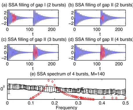
0 100 200
!2 0 2
(a) SSA filling of gap I 12 bursts)
t
0 100 200
!2 0 2
(c) SSA filling of gap II 13 bursts)
t
0 100 200
!2 0 2
t
(b) SSA filling of gap II 12 bursts)
0 0.1 0.2 0.3 0.4 0.5 100
(e) SSA spectrum of 4 bursts, M=140
Frequency
0 100 200
!2 0 2
(d) SSA filling of gap II 14 bursts)
t
Fig. 1. Gap filling of a time series with several identical oscillatory spells (as indicated; in each case only two bursts are shown) and gaps over the interval I: 20≤t≤40 (panel a), and II: 115≤t≤135 (panels b–d); blue line is the original data, red line is the filled-in data (nondimensional units). (e) SSA spectrum of signal with four oscillatory spells (panel d) and windowM=140; red diamonds show SSA eigenvalues, plotted against the dominant frequency as-sociated with the corresponding EOFs; black dots with error bars are the mean and confidence intervals corresponding to the 2.5% and 97.5% percentiles of a Monte Carlo significance test against red noise (Allen and Robertson, 1996).
presented in Section 3 we used 5% of available data and 30 experiments (unless specified otherwise), in order to obtain a smooth estimate of the cross-validation curve and accurate estimates of optimum SSA parameters, with sufficient statis-tical confidence. We will show that this procedure provides reliable estimates of the optimal parametersK∗andMwhen the pattern of missing data is random, though some issues remain in the case of continuous gaps.
To obtain the actual reconstruction, we repeat the inner-and outer-loop iterations, using the optimal parameters ob-tained by cross-validation, but with all the available points now being included in the process.
3 Results
The original idea for using SSA in filling data gaps (R. Vau-tard, pers. commun., 1992) was based on the fact that, in the Toeplitz form of the lag-covariance matrix CX(Vautard and
Ghil, 1989), the constant diagonalscij depend only on the
lag|i−j|and can thus be easily computed from the available data pairs alone. In practice, we have used the Broomhead and King (1986) method for constructing CXfrom the
trajec-tory matrix for all our tests herein. We did so mainly because, in the case of multivariate data, this method automatically includes Beckers and Rixen’s (2003) spatial-EOF–based
re-construction method. The latter corresponds toM=1 in our M-SSA gap filling method and we compare the two cases, of M=1 and M>1, in Sect. 3.2, for global SST data sets. We also carried out a few tests with the Toeplitz form of CX;
these tests did not show any significant difference in our re-sults, though more research can be done on the advisability of either form in various situations.
3.1 Univariate synthetic data
First, we consider a time series consisting of a sinusoidal carrier signal with several periodic, sawtooth-shaped bursts and with synthetic gaps to demonstrate the method’s capa-bilities and limitations on a pure signal without noise. The gap in Fig. 1a lies within the slowly decaying phase of the first sawtooth spell of a time series composed of two such spells, while the gap in Figs. 1b–d masks the rapid excita-tion of the second spell. The period of the carrier signal and the gap size are 5 and 20 sampling units, respectively. The time series plotted in Figs. 1a,b is 230 points long in Figs. 1a,b, while the three and four spells of the complete signals in Figs. 1c,d correspond to 345 and 460 points, respectively. The agreement between the data set filled in by our method and the original time series is almost perfect in Fig. 1a, while in Fig. 1b the period of the signal is captured very well, but not the timing, nor the sharpness of the second spell’s exci-tation. The cross-validated results for choosing SSA param-eters are quite similar in both cases (not shown): the opti-mum number of modes is equal to four; the optiopti-mum window M∗, though, is equal to 10 sampling intervals for the gap in Fig. 1a, and to 20 for Fig. 1b.
The poorer reconstruction result for gap II in Fig. 1b is not surprising, as the time series with two bursts only is too short to use an SSA window that is wide enough to capture the lag correlations required to reconstruct the gap-covering ex-citation phase. When the number of oscillatory bursts in time series increases, the reconstruction dramatically improves, as observed in Figs. 1c, d. The optimum SSA window also be-comes larger, reflecting the long-term periodicity of bursting, and is equal to 140 points for the reconstructions in Figs. 1c, d.
The Monte-Carlo SSA spectrum for the full time series in Fig. 1d (blue line) is shown in Fig. 1e. There is a highly sig-nificant SSA pair representing the main oscillatory mode at the correct frequency of 0.2 unit/cycle, surrounded by a few other pairs, apparently representing the shape of the modu-lated oscillations’ envelope.
For gap filling in Figs. 1b–d we usedK∗=20, which gave the best results and corresponds to the large number of modes necessary to capture the modulations of the spells.
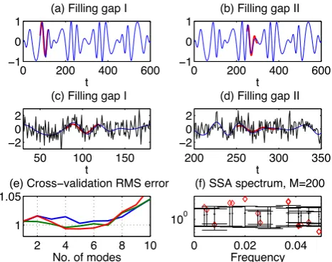
time series x(t) is the signal s(t) contaminated by additive white noise w=w(t), with a normal distribution and a stan-dard deviation equal to one:
x(t )=s(t )+w,
s(t )=sin(2π
200t )·cos( 2π
40t+ π 2sin
2π
120t ). (6)
We apply our SSA gap filling method to both the s(t) and x(t) time series and for intervals I={t:80≤t≤120} and II={t:250≤t≤300}, which correspond to two distinct phases of the nonlinear oscillation.
The filled-in data, shown by the heavy red line in Figs. 2a– d, are in very good agreement with the oscillatory signal s(t) in the gaps, both when noise is present (Figs. 2c, d) and with-out it (Figs. 2a, b). Note that the “noise” modes present in x(t) have been discarded in the reconstruction (Figs. 2c, d). The Monte-Carlo SSA spectra of x(t) in Fig. 2f show six signifi-cant components that correspond to the three pairs associated with the periods 40, 120 and 200; together they capture the nonlinear oscillation. The optimum SSA parameters for gap filling in x(t) are thus suggested by the SSA analysis to be M∗=200, required to capture the longest period present in the time series, andK∗ = 6. This choice is confirmed by the cross-validation in Fig. 2e, which yields a minimum er-ror for M∗=200 andK∗=6; these values turned to be the best choice for gap filling in s(t) as well. The estimate of rms error in reconstruction from the cross-validation is very close to its expected “true” value, equal to unity, which is the standard deviation of white noise in Eq. (6). We tried gaps in other places of the time series, and obtained results similar to those shown in Figs. 2a–d.
3.2 Multivariate geophysical data
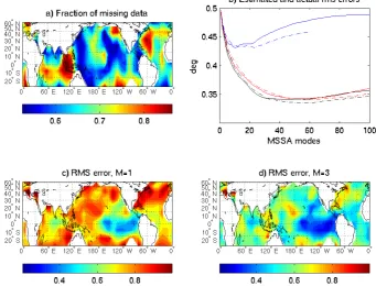
As a first multivariate example, we apply M-SSA gap fill-ing to the global data set of monthly SSTs from the Inter-national Research Institute for Climate and Society (IRI) for 1950–2004, from 30◦S to 60◦N, on a 10◦-latitude by 10◦ -longitude grid, with a total of 660·237=156 420 data points. We have randomly removed about 70% of the data, in a man-ner that is white in time and with spatial correlations that are consistent with the structure of the actually missing SST ob-servations; the fraction of missing observations at each grid point is shown in Fig. 3a. We then applied our iterative gap filling procedure to fill in the missing data, and computed both estimated errors from cross-validation experiments and actual errors in the reconstructed data set.
The cross-validation results in Fig. 3b indicate significant reduction of the rms error when using an optimum window ofM=3 vs.M=1; the latter corresponds to the spatial EOF reconstruction method of Beckers and Rixen (2003). This cross-validation result is verified in Figs. 3c, d by comparing relative error normalized by the standard deviation at each grid point; the errors are indeed much smaller forM=3. The pattern of data missing at random in observed SSTs favors
0 200 400 600
!1 0 1
(a) Filling gap I
t
0 200 400 600
!1 0 1
t
(b) Filling gap II
50 100 150
!2 0 2
t
(c) Filling gap I
200 250 300 350
!2 0 2
t
(d) Filling gap II
2 4 6 8 10
1 1.05
No. of modes
(e) Cross!validation RMS error
0 0.02 0.04
100
(f) SSA spectrum, M=200
Frequency
Fig. 2. Gap filling of (a, b) a nonlinear oscillatory signal s(t), and (c, d) of its noise-contaminated version x(t) (black line); see Eq. (6), units are nondimensional. Blue line is the oscillatory component s(t), red is the filled-in data. Gap I is over the interval 80≤t≤120, while gap II is over 250≤t≤300. (e) Cross-validation results for filling gap II in x(t); blue, green and red lines are for SSA windows ofM=160, 180 and 200, respectively. (f) Monte-Carlo SSA spectra of x(t) with windowM=200 (see caption to Fig. 1).
small M-SSA windows as optimal in reconstruction; we shall see that much larger values ofMare optimal for the substan-tial gaps found in the Nile River and electron flux data sets discussed below.
The influence of the spatial pattern of large signal ampli-tude on the quality of the reconstruction is evident in com-paring Fig. 3d with Fig. 3a: the relative error is uniformly small in the Central and Eastern Tropical Pacific, where the El-Ni˜no/Southern-Oscillation (ENSO) mode dominates seasonal-to-interannual climate variability, despite the low density of data available over part of this area. However, the signal-to-noise ratio is small in the Western Pacific, and the relative error there is larger, despite a comparable fraction of missing data. Estimated errors from cross-validation and the actual absolute errors in the filled-in data set are shown in Fig. 3b by solid and dashed lines, respectively. The curves in each pair are pretty close, thus confirming that the cross-validation procedure provides a good estimate of errors in this case. The rather small difference in absolute errors for M=3 and M=5, despite the large variations in relative er-rors observed in Figs. 3c, d forM=1 andM=3 is due to the higher signal variance in the Eastern Tropical Pacific.
Fig. 3. Reconstruction of missing SST anomaly data for the 50-year-long monthly IRI data set. (a) Fraction of missing data (%); (b) cross-validation results for choosing optimum M-SSA window and number of modes for filling of missing data. Dashed and solid lines are the actual and estimated errors, respectively; blue, black and red colors are for windows ofM=1,M=3, andM=5, respectively. (c, d) Root-mean-square (rms) SST error between the actual and reconstructed SST fields, computed and normalized by the standard deviation at each grid point: (c) for M-SSA windowM=1 and number of modesK∗=10; (d) for optimum M-SSA windowM∗=3 andK∗=50.
rule. Analyzing a complete 1300-yr record of Nile River floods, with the missing points filled in by iterative M-SSA, allowed Kondrashov et al. (2005a) to study the evolution of the record’s regularities over the most recent 450 years (A.D. 1471–1922). In particular, these authors found evidence for a novel source of interannual climatic variability for tropi-cal East Africa, namely changes in the North Atlantic ocean circulation.
Given the fact that high- and low-water records are not always missing the same year, both records were used in fill-ing the gaps in either one (Fig. 4b). Usfill-ing theK∗=9 leading EOFs and a window ofM=100 in the two-channel SSA of high- and low-water levels minimized the estimation error of 50 independent cross-validation experiments. Independent information on the signal-to-noise separation is obtained by inspecting the slope break in the “scree diagram” of SSA eigenvalues for the optimum window M∗=100 (Fig. 4c). There is clear separation between the nine “signal” EOFs that have been used in the reconstruction and the remaining modes, which represent the discarded “noise.”
Our third and last multivariate example is provided by daily measurements of high-energy electron fluxes in Earth’s inner magnetosphere (Fig. 5a) from the Combined Release and Radiation Effects Satellite (CRRES). These observa-tions are 100-day long, and have a total of 100·30=3000
data points, with missing data mainly in the first 80 days of record. In many magnetospheric observations, gaps are present across all the spatial channels, as seen in Fig. 5a on the 64th day; such gaps occur when satellite instruments switch into a different operational mode, or fail due to space hazards. Space physicists are interested in the build-up and relaxation of electron fluxes that coincide with strong, recur-ring geomagnetic disturbances coming from the Sun.
We tested the ability of our algorithm to fill the real gap, as well as three synthetic, continuous gaps of 1 day, 5 day and 3 days, respectively, which we added during strong magnetic storms (Fig. 5b). The reconstruction error for synthetic gaps, presented in Fig. 6, shows that the optimum M-SSA window width and number of modes is equal toM∗=30 andK∗=19, respectively.
!00 1000 1200 1400 1600 1!00 !4
!20 2 4
(a) O+,-,.a/ +0c2+34
50a+ 6A8)
!00 1000 1200 1400 1600 1!00
!4 !20 2 4
50a+ 6A8)
(b) :!;;A <,//03 ,.
0 5 10 15 20 25 >0
100
102
(c) :!;;A 4?0c@+AB 2< <,//03 N,/0 R,E0+ +0c2+34F :G100
N2. 2< B2304
Fig. 4. Extended records (A.D. 622–1922) of low-water (solid black curve) and high-water (solid red) levels: (a) original data; and (b) data with missing points filled in by M-SSA. The gap filling uses a window ofM=100 yr and two channels (the low- and high-water levels). The time series have been centered on the relevant mean and the amplitudes have been normalized by the standard devia-tion of the original time series (excluding missing data points). The mean of the high-water record is 907 cm, while it is 288 cm for the low-water record; the corresponding values for the variances are 6586 cm2 for the high-water record and 10 359 cm2 for the low-water record. (Panels (a) and (b) reproduced from Kondrashov et al., 2005a, by permission of the American Geophysical Union). (c) M-SSA spectrum of filled Nile River records,M∗=100 years. The optimum numberK∗=9 of modes corresponds to the break in the slope of the M-SSA spectrum.
When continuous gaps are present at all spatial locations over some time interval, using a window widthM>1 allows one to reduce the reconstruction error significantly in com-parison with purely spatial EOF reconstruction (M=1). In the latter case, missing data in the gaps are replaced with a constant time-mean value at a particular grid point. In con-trast, forM>1, cross-channel, time-lagged spatial correla-tions are taken into account. This feature of the method en-sures temporal variations and lower rms errors in the gaps.
Some challenges do remain in using cross-validation to choose optimum SSA parameters for the case of continuous gaps in multivariate data, as well as for time series with “red” temporal spectra (see Sect. 2.2). For example, the true recon-struction errors forM=1 will not depend on the number of EOFs retained, as shown in Fig. 6. Randomly deleting points for cross-validation may, however, not capture correctly the actual error level in continuous gaps. Filled-in data at ran-domly chosen points, at a given time moment, will take into account spatial correlations from existing values at other grid points, leading to the rms error being reduced as more signal modes are added in the reconstruction. Using gappy time in-tervals for cross-validation improves the estimate of actual
L
(a) Satellite data
10 20 30 40 50 60 70 80 90 100
10 20 30
!2 !1 0
L
(b) Satellite data with gaps added
10 20 30 40 50 60 70 80 90 100
10 20 30
!2 !1 0
Days
L
(c) M!SSA filled in
10 20 30 40 50 60 70 80 90 100
10 20 30
!2 !1 0
Fig. 5. CRRES satellite measurements of 1MeV high-energy elec-tron fluxes (sr·MeV·s·cm2)−1in Earth’s radiation belts as a func-tion of L-shell: (a) original data with missing values in white; (b) original data with a few synthetic gaps added; and (c) M-SSA filled-in. The L-shell parameter measures distance to the intersection be-tween a magnetic-dipole field line and the equatorial plane in Earth radii; it indicates how far trapped electrons are from the Earth.
0 10 20 30 40 50 60
0.25 0.3 0.35 0.4 0.45 0.5 0.55 0.6 0.65
M!SSA -o/es
(sr
!
Me4
!
s
!
c-2 )
!
1
7econstr:ction error for synthetic gaAs
M=1 M=20 M=30 M=40
Fig. 6. RMS reconstruction error for synthetic gaps in the CRRES satellite data set of electron fluxes (Fig. 5c), as a function of window widthMand numberKof M-SSA modes.
1"55 1"60 1"65 1"&0 1"&5 1""0
!6
!4
!2 0 2 4 6
)*a,
Index
/OA23 /R5
/OA23!33A//R5 /OA23!33A /R5!733A /OA23!733A
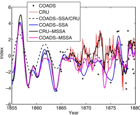
Fig. 7. Reconstruction of pre-1880 SOI time series. Different methods are applied to the COADS data set, with or without CRU data as well: original COADS data (asterisks), CRU SOI (red line); filled-in COADS: with SSA conditioned on CRU (black dashed line), with SSA of COADS data only (blue line), with M-SSA us-ing jointly the COADS and CRU data (solid magenta); and recon-structed CRU with optimal M-SSA parameters (solid black).
3.3 Comparison of different methods
To compare the performance of our iterative SSA method with other ways of filling gaps in time series, we consider for simplicity a univariate data set. This is provided by the monthly values of the Southern Oscillation Index (SOI) for 1854–1997, from the Comprehensive Ocean-Atmosphere Data Set (COADS; Woodruff, 1987), available from http:// tao.atmos.washington.edu/data/soicoads2/ and derived from ship observations. The SOI is based on the mean sea level pressure difference between Tahiti, French Polynesia, and Darwin, Australia (Tahiti-Darwin); the SOI represents the atmospheric signature of a coupled ENSO oscillatory mode. Many SOI data are missing, especially in the early part of the record (1854–1880), which we reconstruct using our SSA gap-filling procedure. Our reconstructions are then com-pared with the SOI time series from the Climatic Research Unit (CRU) at East Anglia University (1866–1997), available at http://www.cru.uea.ac.uk/ftpdata/soi.dat, and based on the Ropelewski and Jones (1987) data.
First, three data points with unreasonably large values (greater than 5) have been flagged as missing in the earlier part of the COADS data set. Then we tried different gap fill-ing strategies. First, we applied SSA reconstruction to the COADS data, but with the cross-validation error computed against CRU data, wherever it overlaps with missing COADS data, which is mainly during the 1870–1880 time interval. The minimum of the corresponding rms error occurs for a windowM∗=60 andK∗=2 modes. The filled-in time series
with these parameters is shown in Fig. 7 as a black dashed line.
Next we applied regular SSA reconstruction to the COADS data alone, as in the previous examples of Sects. 3.1 and 3.2. The minimum cross-validation error corresponds in this case to a windowM∗=100 andK∗=12 modes; the re-constructed data is shown by the blue line. Finally, we use the CRU and COADS time series together, and applied M-SSA reconstruction to take advantage of existing correlations be-tween the two time series. Cross-validation yields a window ofM∗=100 and K∗=27 modes as optimal M-SSA param-eters. The reconstruction is shown by the magenta line and the corresponding “CRU channel” of the M-SSA reconstruc-tion is shown by a black solid line; as expected, the latter follows quite closely the raw CRU data, except for its being somewhat smoother, due to the use ofK∗=27 modes.
All the COADS reconstructions in pre-1870 years are dominated by an oscillatory mode with a period of about 4 yr, and are in fairly good agreement with each other. Signifi-cant differences exist, however, during the years 1868–1878, depending on whether and how we used the CRU data in this time interval. Reconstruction with the minimum distance from CRU time series passes quite far from the few existing COADS points. On the other hand, the SSA reconstruction using only the COADS data passes closer to these points, as expected. The COADS reconstruction by two-channel M-SSA lies somewhere in the middle.
Fairly different reconstructions can thus be obtained when independent data sources exist, all of which may provide consistent fits to some portion of the data that the sources have in common. The question of which SOI reconstruction should be trusted more can only be settled as additional data or additional theoretical insights become available.
4 Conclusions
Iterative SSA is a new and promising method to fill gaps in a considerable variety of geophysical records. The gaps may be distributed at random in space and time, or they may con-tain patches of data missing in space, as well as windows of data missing in time. The accuracy and reliability of the method depend on the pattern of missing data, the relative length of the gaps with respect to the total length of the data set, and the fraction of variance captured by robust, oscilla-tory modes.
The SOI example in Sect. 3.3 involved extension of the time series into the past. It is clear, though, that our iterative SSA gap filling may be used just as well for extending the series into the future, i.e. for prediction. We plan to explore this aspect of the method’s capabilities further, comparing it with other statistical or mixed statistic-dynamical forecast methods (Ghil and Jiang, 1998; Kondrashov et al., 2005b). Acknowledgements. It is a pleasure to thank R. Vautard for the original suggestion of using the Toeplitz form of the lag-covariance matrix in the presence of data gaps. D. Percival and T. De Putter kindly provided several sets of Nile River records in digitized form; see Kondrashov et al. (2005a) for details. We are also grateful to Y. Shprits for providing the CRRES measurements and for useful discussions. This work is supported by NSF grant ATM00-81231.
Edited by: M. Thiel
Reviewed by: A. Y. Schumann and another referee
References
Allen, M. R. and Robertson, A. W.: Distinguishing modulated oscil-lations from coloured noise in multivariate datasets, Clim. Dyn., 12, 775–784, 1996.
Alvera-Azc´arate, A., Barth, A., Rixen, M., and Beckers, J. M.: Re-construction of incomplete oceanographic data sets using empiri-cal orthogonal functions: applications to the Adriatic Sea surface temperature, Ocean Modelling, 9, 325–346, 2005.
Beckers, J. and Rixen, M.: EOF calculations and data filling from incomplete oceanographic data sets, J. Atmos. Ocean. Technol., 20, 1839–1856, 2003.
Broomhead, D. S. and King, G. P.: Extracting qualitative dynamics from experimental data, Physica D, 20, 217–236, 1986. Colebrook, J. M.: Continuous plankton records: zooplankton and
environment, North-East Atlantic and North Sea, 1948–1975, Oceanol. Acta, 1, 9–23, 1978.
Dettinger, M. D., Ghil, M., Strong, C. M., Weibel, W., and Yiou, P.: Software expedites singular-spectrum analysis of noisy time series, Eos, Trans. American Geophysical Union, v. 76(2), p. 12, 14, 21, 1995.
Foster, G.: Wavelets for period analysis of unevenly sampled time series, Astronom. J., 112, 1709–1729, 1996.
Fraedrich, K.: Estimating the dimensions of weather and climate attractors, J. Atmos. Sci., 43, 419–432, 1986.
Ghil, M. and Vautard, R.: Interdecadal oscillations and the warming trend in global temperature time series, Nature, 350, 324–327, 1991.
Ghil, M. and Jiang, N.: Recent forecast skill for the El Ni˜no/Southern Oscillation, Geophys. Res. Lett., 25, 171–174, 1998.
Ghil, M., Allen, R. M., Dettinger, M. D., Ide, K., Kondrashov, D., et al.: Advanced spectral methods for climatic time series, Rev. Geophys. 40(1), 3.1–3.41, doi:10.1029/2000RG000092, 2002.
Johns, C., Nychka, D., Kittel, T., and Daly, C.: Infilling sparse records of spatial fields, J. Amer. Stat. Assoc., 98(464), 796–806, 2003.
Kaplan, A., Kushnir, Y., Cane, M., and Blumenthal, M.: Reduced space optimal analysis for historic data sets: 136 years of At-lantic sea-surface temperatures, J. Geophys. Res., 102, 27 835– 27 860, 1997.
Kondrashov, D., Feliks, Y., and Ghil, M.: Oscillatory modes of ex-tended Nile River records (A.D. 622–1922), Geophys. Res. Lett., 32, L10702, doi:10.1029/2004GL022156, 2005a.
Kondrashov, D., Kravtsov, S., and Ghil, M.: A hierarchy of data-based ENSO models. J. Climate, 18, 4425–4444, 2005b. MacDonald, G. J.: Spectral analysis of time series generated by
nonlinear processes, Rev. Geophys., 27, 449–469, 1989. Mann, M. E., Bradley, R. S., and Hughes M. K.: Global-scale
tem-perature patterns and climate forcing over the past centuries, Na-ture, 392, 779–787, 1998.
Mendelssohn, R., Schwing, F. B., and Bograd S. J.: Spatial structure of subsurface temperature variability in the Califor-nia Current, 1950–1993, J. Geophys. Res., 108(C3), 3093, doi:10.1029/2002JC001568, 2003.
Popper, W.: The Cairo Nilometer, 269 pp., University of California Press, Berkeley/Los Angeles, 1951.
Reynolds, R. W. and Smith, T. M.: Improved global sea-surface temperature analysis using optimum interpolation, J. Climate, 7, 929–948, 1994.
Ropelewski, C. F. and P. D. Jones: An extension of the Tahiti– Darwin Southern Oscillation Index, Mon. Wea. Rev., 115, 2161– 2165, 1987.
Schneider, T.: Analysis of incomplete climate data: Estimation of mean values and covariance matrices and imputation of missing values, J. Climate, 14, 853–871, 2001.
Schoellhamer, D.: Singular spectrum analysis for time series with missing data, Geophys. Res. Lett., 28(16), 3187–3190, 2001. Schulz, M. and Mudelsee, M.: REDFIT: estimating red-noise
spec-tra directly from unevenly spaced paleclimatic time series, Com-puters and Geosciences, 28, 421–426, 2002.
Sherwood, S.: Climatic signals from station arrays with missing data, and an application to winds, J. Geophys. Res., 105, 29 489– 29 500, 2000.
Smith, T. M., Reynolds R. W., Livezey R. E., and Stokes D. C.: Reconstruction of historical sea-surface temperatures using em-pirical orthogonal functions, J. Climate, 9, 1403–1420, 1996. Toussoun, O.: M´emoire sur l’histoire du Nil, M´emoires de l’Institut
d’Egypte, 18, pp. 366–404, Cairo, 1925.
Varadi, F., Pap, J. M., Ulrich, R. K., Bertello, L., and Henney, C. J.: Searching for signal in noise by random-lag singular spectrum analysis, Astrophys. J., 526, 1052–1061, 1999.
Vautard, R. and Ghil, M.: Singular spectrum analysis in nonlinear dynamics, with applications to paleoclimatic time series, Physica D, 35, 395–424, 1989.