2MARUM – Center for Marine Environmental Sciences, Bremen, Germany
3AWI – Alfred Wegener Institute for Polar and Marine Research, Bremerhaven, Germany Correspondence to:Nikolay V. Koldunov ([email protected])
Received: 3 January 2017 – Discussion started: 31 January 2017
Revised: 15 August 2017 – Accepted: 27 August 2017 – Published: 29 September 2017
Abstract. Satellite sea ice concentrations (SICs), together with several ocean parameters, are assimilated into a regional Arctic coupled ocean–sea ice model covering the period of 2000–2008 using the adjoint method. There is substantial im-provement in the representation of the SIC spatial distribu-tion, in particular with respect to the position of the ice edge and to the concentrations in the central parts of the Arctic Ocean during summer months. Seasonal cycles of total Arc-tic sea ice area show an overall improvement. During sum-mer months, values of sea ice extent (SIE) integrated over the model domain become underestimated compared to observa-tions, but absolute differences of mean SIE to the data are reduced in nearly all months and years. Along with the SICs, the sea ice thickness fields also become closer to observa-tions, providing added value by the assimilation. Very sparse ocean data in the Arctic, corresponding to a very small con-tribution to the cost function, prevent sizable improvements of assimilated ocean variables, with the exception of the sea surface temperature.
1 Introduction
The Arctic region is expected to experience a dramatic an-thropogenic temperature increase over the years to come (IPCC, Stocker et al., 2014). A major decline in Arctic sea ice is already observed (Kwok and Rothrock, 2009; Comiso et al., 2008) and climate change projections suggest that, due to rising temperatures, a complete disappearance of summer sea ice could occur as soon as 2050 (Overland and Wang, 2013). Obtaining an improved understanding of the
chang-ing Arctic Ocean, its transport properties of heat, freshwater and carbon and nutrients, and its interaction with sea ice and the overlying atmosphere is therefore of utmost importance.
Despite recent improvements in observing capabilities (Lee et al., 2010), the Arctic Ocean remains one of the least explored areas of the world ocean. This is due both to the harsh environmental conditions of the region and logisti-cal and politilogisti-cal difficulties in maintaining sustained Arctic-wide, ideally autonomous, ocean observations. Fortunately, many polar-orbiting satellites obtain important ocean and sea ice parameters over the sub-Arctic region, such as sea surface height (SSH), sea surface temperature (SST), ocean color and sea surface salinity (SSS). However, over sea-ice-covered re-gions satellite measurements of the ocean surface are lim-ited. To enhance our insight into the Arctic environment a joint analysis of observational efforts is therefore required. However, to understand large-scale circulation processes in the Arctic Ocean the community will have to rely on numeri-cal ocean circulation models due to the continued substantial undersampling of the Arctic under sea ice cover.
The representation of the Arctic Ocean circulation in ex-isting ocean models considerably improved during the last 10 years, to the point that today many models reproduce the variability of SSH reasonably well (Koldunov et al., 2014), while for the components of the freshwater balance the pic-ture is mixed (Jahn et al., 2012) and for circulation and wa-ter mass models show significant discrepancies (Proshutin-sky et al., 2011).
conclu-sions about variations in Arctic Ocean parameters on decadal scales and to reveal mechanisms which drive changes in Arc-tic circulation.
Stammer et al. (2016) described the state of ocean data as-similation in the context of climate research. As described there, ocean data assimilation became a mature field for the ice-free ocean. However, assimilation in coupled ocean–sea ice or fully coupled climate models is still at its infancy and needs considerable attention. This also includes the use of sea ice parameters to constrain coupled ocean–sea ice mod-els and to understand the coupling between sea ice and the underlying ocean and the atmosphere.
(Chevallier et al., 2016) recently reported results from the ORA-IP inter-comparison project for Arctic sea ice parame-ters using global ocean–sea ice reanalyses with and without assimilation of sea ice data. They found good agreement in the reconstructed concentration but a large spread in sea ice thickness (SIT) due to biases related to the sea ice model components.
The approaches to the sea ice assimilation are similar to the way ocean variables are assimilated in ocean models and range from nudging (e.g., Lindsay and Zhang, 2006; Ti-etsche et al., 2013) to the use of ensemble Kalman filter (e.g., Lisæter et al., 2003; Xie et al., 2016). The sea ice sensitivity study of Koldunov et al. (2013) was among the first prereq-uisites to a full data assimilation attempt in the Arctic with the adjoint method. The authors looked at the sensitivity of sea ice parameters to external atmospheric forcing parame-ters (see also Kauker et al., 2009). The former study revealed the impact of spring atmospheric temperatures on summer sea ice concentration (SIC) and extent. The study of Kauker et al. (2009) underlined that wind stress changes are impor-tant for changing summer SIT.
More recently, Fenty et al. (2015) studied the impact of assimilating SIC (and ocean) data into a global, eddy-permitting ocean circulation model using the adjoint method. In that study the circulation for the year 2004 was recon-structed. By comparing a setup with and without assimilation of SIC, the authors demonstrate that SIC data reduce model misfits in the Arctic with respect to upper ocean stratification and reduces ICESat-derived Arctic ice thickness errors.
The present study builds on the work of Fenty et al. (2015) and advances it by performing a multi-year data assimilation for the coupled Arctic Ocean–sea ice system. To be compu-tationally feasible, the study is based on a regional Arctic configuration, nested laterally into a North Atlantic–Arctic solution (Serra et al., 2010). The goal of the study is to inves-tigate the changes in the Arctic during the period of 2000– 2008. This period is characterized by significant changes in the Arctic Ocean and by increased amounts of Arctic obser-vations. This makes it a good test period for the assimilation system and can provide first scientific applications. At the same time, the consistency of the assimilated EUMETSAT sea ice data (OSI-SAF, 2015) with the used sea ice model is being tested, as are its impact on the estimate of the ocean
circulation and unobserved ice parameters such as sea ice thickness.
The remaining paper is structured as follows: after an in-troduction to the model configuration and the assimilation method in Sect. 2, the impact of the assimilation on the SIC is discussed in Sect. 3. Section 4 focuses on how the sea ice state is adjusted by changing the control variables and Sect. 5 summarizes the impact on the ocean state and the sea ice thickness. Concluding remarks follow in Sect. 6.
2 Methods
Our study is based on a regional configuration of the MIT-gcm coupled ocean–sea ice model (Marshall et al., 1997) and the respective ECCO adjoint framework. The model setup, the data assimilation and the optimization results are de-scribed in the following subsections.
2.1 Model setup
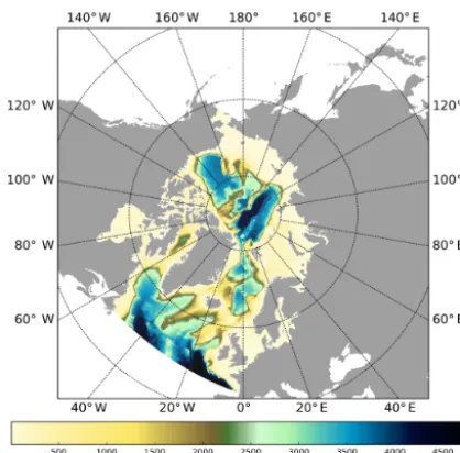
The model domain covers the northern North Atlantic and the Arctic Ocean (Fig. 1) with the model grid being curvi-linear and a subset of the 16 km resolution Atlantic–Arctic model (ATL06) reported in Serra et al. (2010). The model useszcoordinates and has 50 levels, with resolution varying from 10 m in the top layers of the water column to 550 m in the deep parts of the ocean. The bathymetry is based on the ETOPO2 database (Smith, 1997) with no artificial deepening or widening of the Nordic Seas’ passages being applied.
Figure 1.Model domain with bathymetry.
thermodynamic sea ice model. The thermodynamic part of the model is the so-called zero-layer formulation following Semtner (1976) with snow cover as in Zhang et al. (1998). The temperature profile in the ice is assumed to be linear, with constant ice conductivity. Such a formulation implies that the sea ice does not store heat, and, as a result, the sea-sonal variability of sea ice is exaggerated (Semtner, 1984). To reduce this effect we use the sub-grid-scale heat flux pa-rameterization following Hibler (1984). Moreover, we use the viscous–plastic rheology scheme of Hibler (1979) with an extended line successive over-relaxation (LSOR) method (Zhang and Hibler, 1997). A comparison of the effect of dif-ferent rheology schemes in MITgcm is provided by Losch et al. (2010). Recently, Nguyen et al. (2011) applied the cou-pled MITgcm in a regional Arctic Ocean study and reported values for many model parameters used in our study. 2.2 Adjoint data assimilation approach
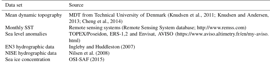
Similar to the work of Fenty et al. (2015), our assimilation also employs the ECCO adjoint methodology to bring the coupled sea ice–ocean general circulation model into con-sistency with assimilated data and prior uncertainties. The particular implementation used here builds on the setup of the GECCO2 synthesis (Köhl, 2015) but was extended to fa-cilitate the additional assimilation of sea ice parameters. A complete list of parameters assimilated and their sources is presented in Table 1. The collection of hydrographic obser-vational data in the Arctic Ocean used in the present work is not comprehensive and does not include, for example, ice-tethered profiler data (Toole et al., 2011; Krishfield et al., 2008). In the present pilot study we decided to stick to two well-structured data sets available at the time we started our efforts.
tween the first-guess initial condition and the model state at the beginning of the assimilation period (only for the first year), andumis the difference between the first-guess time mean atmospheric state and the optimized mean atmospheric state, ua(t ) is the difference between the first-guess time-varying atmospheric state and the optimized time-time-varying at-mospheric state. Additional weightsR(t )−1, P(0)−1, Q−1m and Qa(t )−1 control the relative contribution of different terms in the cost function. A more detailed description of the cost function and optimization procedure can be found in Fenty et al. (2015).
The MITgcm is suitable for the automatic generation of adjoint code by the Transformation of Algorithms in FORTRAN (TAF) source-to-source translator (Giering and Kaminski, 1998; Giering et al., 2005). Koldunov et al. (2013) used the MITgcm and its adjoint to perform an analysis of the Arctic-wide adjoint-based sea ice sensitivities to atmospheric forcing.
Table 1.Data sets used in the assimilation procedure.
Data set Source
Mean dynamic topography MDT from Technical University of Denmark (Knudsen et al., 2011; Knudsen and Andersen, 2013; Cheng et al., 2014)
Monthly SST Remote sensing systems (Remote Sensing System database; http://www.remss.com)
Sea level anomalies TOPEX/Poseidon, ERS-1,2 and Envisat, AVISO (https://www.aviso.altimetry.fr/en/my-aviso. html)
EN3 hydrographic data Ingleby and Huddleston (2007) NISE hydrographic data Nilsen et al. (2008)
Sea ice concentration OSI-SAF (2015)
In contrast to Köhl (2015), additional control variables are optimized and the frequency of the updates is enhanced to once per 3 days in order to reflect shorter timescales of sea ice variability. The final list of control variables is sur-face (2 m) air temperature, sursur-face (2 m) specific humidity, surface (10 m) zonal and meridional wind velocity, precipi-tation rate, downward shortwave radiation, and initial tem-perature and salinity for the first year of assimilation. For the atmospheric control variables, uncertainties were speci-fied as the maximum of the standard deviation of the NCEP fields for the 1948–2008 time period and the errors for the mean components of air temperature, humidity, precipita-tion, downward shortwave radiation and wind were specified as 1◦C, 0.001 kg kg−1, 1.5×10⁻⁸mm s−1, 20 W m−2 and 2 m s−1, respectively. For the downward shortwave radiation both mean and time-varying parts were set to 20 W m−2.
We employ the same uncertainty weights for hydrographic and satellite data as Köhl (2015), while for sea ice concen-tration we specify a constant error of 50 %. We verified the sensitivity of our results by using space–time-varying sea ice uncertainty estimates as they became available, as well as different values of a constant error. Results of the sea ice as-similation with variable uncertainties were very similar to the ones with a constant error value of 50 %.
The data assimilation is performed in 1-year chunks. The use of 1-year segments is related to technical reasons; we are not able to get useful sensitivities for the time period longer than a year for all years of our 2000–2008 assimilation pe-riod. We were successful in completing a 2-year assimilation at one occasion (2005–2004), but the results for sea ice area (SIA) and thickness were not noticeably different from the 1-year chunk assimilation.
Each of the iterative cost function reductions is performed until the cost function differs by less than 1 % in two consec-utive iterations. The cost is dominated by SIC and SST data, which easily respond to the surface controls, and the adjoint method quickly reduced the misfits of those data, so that the number of iterations was usually less than five (it is three iterations for 2000, 2003, 2004, 2005, 2006 and 2007, four iterations for 2002 and 2008 and five iterations for 2001). After the first year assimilation, we move to the next year
using the final state of the previous year’s successful itera-tion as initial condiitera-tions. Therefore, the iteraitera-tion termed 0 in the following makes already use of an improved initial con-dition from the assimilation in the previous year and is thus not equivalent to a free run starting from climatology. For the impact on the ocean circulation, we consider also the free run to demonstrate the impact of changing the initial conditions by assimilating data during the preceding year.
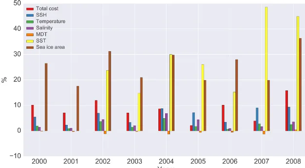
Figure 2 shows the percentage decrease in model–data dif-ferences. The red color indicates reduction in total model– data difference, while other colors indicate the reduction of the differences for individual variables. Negative values mean that there is an increase in model–data difference for that variable.
The largest total reduction (about 16 %) is obtained for the year 2008, while the smallest (about 2 %) is obtained for the year 2005. The average reduction for all years is about 9 %. The strongest cost reductions for individual variables is ob-tained for the SST and SIA, with an overall average of about 23 and 26 %, respectively. The least successful cost reduc-tion is obtained for the mean dynamic topography (MDT), with many years in which the model–data differences for this variable slightly increased. In 2004 the cost reduction of sea ice area was about 30 %, less than that reported by (Fenty et al., 2015) (49 %), which may partly be explained by dif-ferences in the first-guess solution.
Taking into account differences in the amount of sea ice concentration and sea surface temperature data compared to the amount of hydrography data, it is not surprising that most of the contributions to the total reduction of the cost function are from SIC and SST. Hence most of the improvements can be expected to happen in these fields, while changes in the state of the ocean is expected to be small.
In the following we concentrate mainly on results related to changes of the sea ice conditions, with only a brief discus-sion of ocean state changes later on.
3 Sea ice concentration changes
Figure 2.Total cost reduction and individual contributions to the reduction from different assimilated variables. During the first 2 years SST assimilation is not performed (no data).
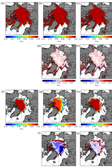
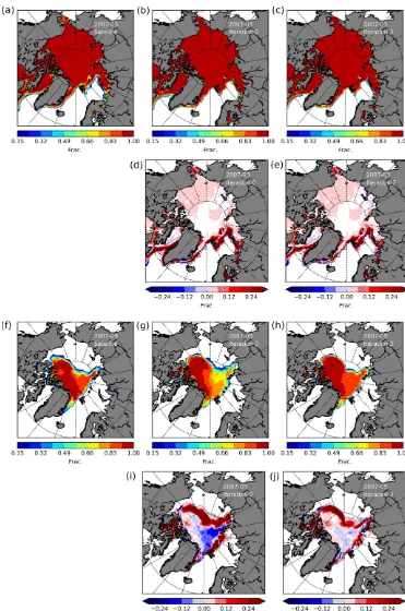
satellite and from model runs, before and after data assimi-lation, together with the changes of the latter two relative to observations. Since most of the Arctic Ocean is covered by sea ice with high concentrations, the largest improvements are in the position of the ice edge. Most noticeable is the de-crease in the SIC along the east coast of Greenland after data assimilation. During the initial run of the model, there is a tongue of the sea ice extending towards the open ocean. Af-ter data assimilation the tongue did not disappear completely, but it declined considerably.
During the summer period (September 2005), shown in the bottom two rows of Fig. 3, there are improvements both in the sea ice edge and in the SIC of the interior sea ice field. Initially, the sea ice edge was not very far from observations, but after data assimilation the match between model and data is improved. The SIC in the central parts of the Arctic Ocean increased and became closer to the satellite data. A direct comparison to the results by Fenty et al. (2015) is hindered by the fact that differences less than 15 % are blanked out in their study and by the different years analyzed.
In order to test the consistency of the estimate with the ob-servations and the uncertainties we compare the spatial dis-tribution of monthly mean sea ice concentration absolute dif-ferences before and after data assimilation to the maps of spatial distribution of monthly mean total standard error in the ESA SICCI sea ice concentration product (ESA SICCI, 2013). The latter provide daily spatially varying estimates of sea ice concentration errors. The absolute differences after assimilation correspond well to the total standard error spa-tially and by value with only few spots along the edges with very high absolute differences (not shown).
In contrast to 2005, identifying changes in the SIC for March 2007 (Fig. 4) is more challenging. Practically all the differences between simulations and satellite data are along the ice edge and there seems to be not much change between
the initial state of the model and the state after assimila-tion. For example, the noticeable negative anomaly around Franz Joseph Land is not developed further after SIC assim-ilation. This particular negative SIC anomaly is most prob-ably dynamical in nature and cannot be handled properly by the simplified ice dynamics scheme (free drift) used in the adjoint model to calculate changes of the model parame-ters. The spatial distribution of SIC during September 2007 (Fig. 4) already bears a good resemblance to the satellite data before the assimilation. Improvements are mostly visi-ble in the central parts of the Arctic Ocean, where the too-low SIC is increased. The ice edge also became closer to obser-vations, but the amount of sea ice in the Amerasian basin remains larger compared to observations. In this region the SIC in the unconstrained run is high (with also thicker sea ice), which is not easy to remove by thermodynamic correc-tions of the forcing and, due to the high SIC and thickness, not easy to move by changes in wind forcing. This possibly indicates some limitations of the approach, where the correc-tions mostly come from the thermodynamic forcing and the assimilation period is short.
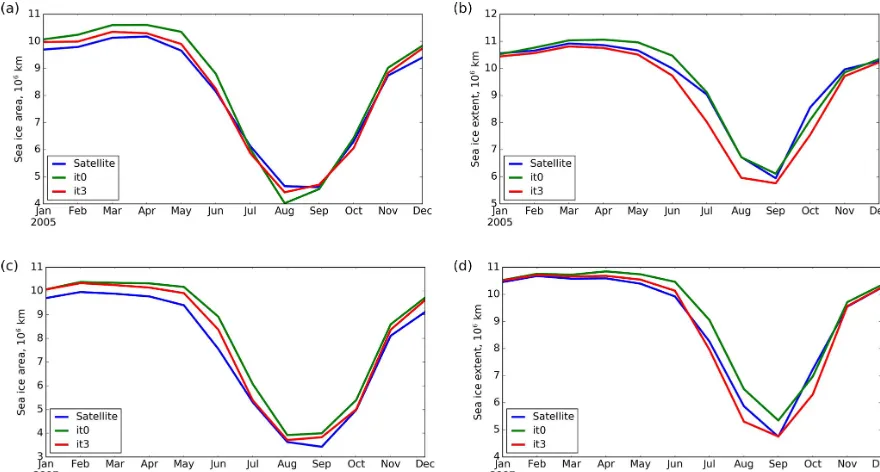
Figure 5.Monthly mean sea ice area(a, c)and extent(b, d)for the years 2005(a, b)and 2007(c, d). Assimilated satellite data is shown in blue, and model solution without corrections is shown in green and the result from the last iteration is shown in red.
For both years, SIA shows overall improvement during the whole year, but this is not the case for the SIE. In 2005 the SIE good match between initial iteration and satellite data during summer months disappears after assimilation, with considerable underestimation of SIE. In 2007 there is an overall SIE improvement after the assimilation, but there are again months with a considerable SIE underestimation. Both metrics suffer from the inability to guarantee that improve-ments in this metric also lead to an overall improved match in the spatial sea ice coverage, since a perfect total SIA or SIE evolution may still correspond to considerable differences to the data in their regional distribution. Chances of having SIE distribution close to observations with quite different spa-tial shape of the sea ice field are very high. This calls for changing the common practice of model evaluation by only comparing their ability to simulate present day SIE without considering the sea ice spatial distribution (e.g., Dukhovskoy et al., 2015).
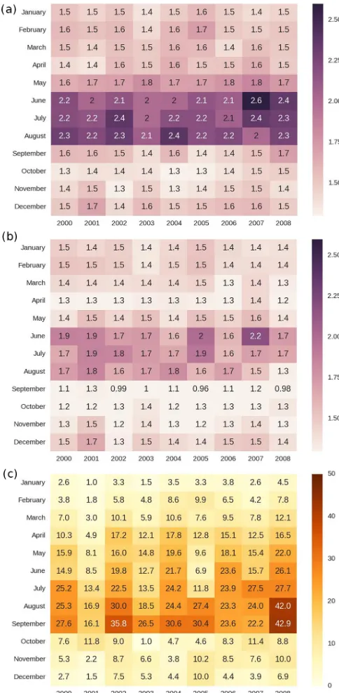
With respect to the model performance, two better met-rics are the sum of absolute differences (SoAD) for SIA and SIE, which at least to some extent consider differences in spatial distribution by penalizing positive and negative differences at every grid point. Monthly values of the SIA SoAD before assimilation, after assimilation and the respec-tive differences between the two (in percent) are shown in Fig. 6. Before assimilation, largest SoAD appear during sum-mer months (>2×10⁶km2), while in other seasons they are about 1.5×10⁶km2. Interesting to note, values of SoAD in March and September are quite similar, despite the large differences in ice cover in the 2 months. One of the
possi-ble reasons is that location of the ice edge in those extreme months is relatively stable compared to spring and fall when the ice pack is contracting and expanding. After the assimi-lation the most notable improvements also occur for summer months, but with the addition of September. After the assim-ilation, March values show only about 10 % improvement, while September values have about 25 % improvement on average. There is no clear indication that assimilation of SIC on the yearly basis gradually improves the simulated sea ice due to, for instance, better initial conditions in January. For some months the decrease in SIA SoAD after assimilation can be as little as 1 %, although it is always getting smaller. The same is not the case for the SIE SoAD.
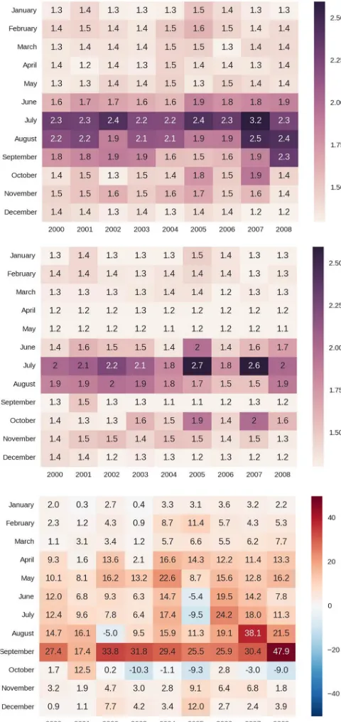
As expected, SIE SoAD values (Fig. 7) are larger, with a maximum in summer and September before the data assim-ilation. Assimilation is most effective for a reduction of SIE SoAD in September (about 25 % on average). After the as-similation October becomes, in addition to summer months, one of the months with relatively large SIE SoAD differ-ences. October is also a month when (during 5 out of 9 years) after assimilation the SIE SoAD increased. The SIE SoAD, similarly to the SIA SoAD, do not show any obvious ten-dency from the first year to the last.
4 Control variables
opti-Figure 6.Sum of the sea ice area absolute differences (SoAD) com-pared to assimilated sea ice at every grid location, for every month (in 106km2), before assimilation(a), after assimilation(b)and the percent difference between the two(c). Positive differences corre-spond to a decrease of SoAD.
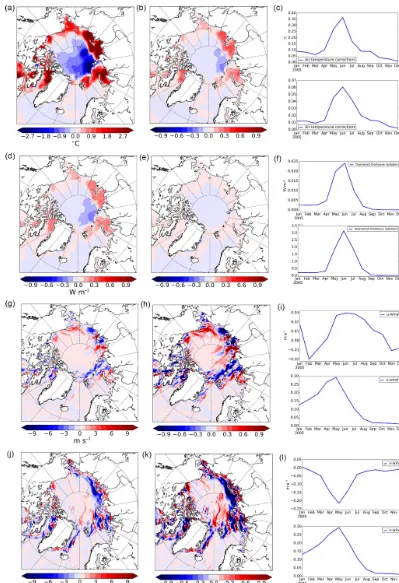
mization procedure changes the forcing and the initial con-ditions in order to bring the state of the model closer to the observed state. Figure 8 shows the area-mean temporal vari-ation of the corrections to several control variables over the year 2005 in absolute values and normalized by the
uncer-months (not shown).
The corrections to the downward shortwave radiation (Fig. 8, second row) show temporal variations and a spatial distribution similar to the SAT corrections, but the magni-tudes are quite small. Corrections to the zonal and merid-ional wind components (Fig. 8, third and last rows) are on average quite small in absolute values but locally can reach 10 m s−1. The wind corrections are mainly concen-trated along the shore and summer ice edge and, contrary to the SAT corrections, it is difficult to associate them with some particular large-scale sea ice change.
Dimensional values of the corrections do not directly pro-vide information about the relative importance of changes in the controls for bringing the model into consistency with ob-servations. However, due to the relatively small number of iterations, we can use values of the corrections normalized by uncertainties as a reasonable measure of the relative im-portance of changes in control parameters. Spatial distribu-tions and monthly means of absolute values of normalized corrections for the year 2005 are shown in Fig. 8.
Wind corrections seem to play integrally a larger role, with a maximum in May. This agrees well with results of Kauker et al. (2009), who used an adjoint sensitivity analysis to de-termine the relative contribution of different atmospheric and ocean fields to the September 2007 sea ice minimum and found that the May–June wind conditions are one of the main factors in setting up extremely low sea ice conditions in sum-mer 2007. The maximum contribution of air temperature cor-rections occurs in June and it is about a factor of 5 smaller than the contribution of the wind corrections. However, using free drift in the adjoint biases the sensitivities towards larger sensitivities of sea ice to wind changes. Since measuring the impact by the normalized corrections relies on the assump-tion of correct sensitivities, the results may be also biased to too large an impact by the wind.
Figure 7.Same as Fig. 6, but for the sea ice extent.
particularly since in the Arctic the NCEP reanalysis seems to perform well near the surface (Jakobson et al., 2012). For example, temperatures decreasing over areas with high SIC during summer months in order to grow ice and tempera-tures increasing over low SIC areas could be an attempt of the assimilation system to fix problems associated with the sea ice movement. However, it could equally also point to problems of the correct attribution of sea ice concentrations
from satellite data. In both cases, corrections to atmospheric control variables will not improve the quality of the original atmospheric forcing but may actually make it worse.
5 Improvements in sea ice thickness and ocean state
The adjoint assimilation leads to dynamically consistent model solutions, which along with directly assimilated vari-ables may considerably improve varivari-ables of the simulation for which no observations are available. In case of SIC assim-ilation, one obvious candidate for improvement is the SIT. We also consider changes in the ocean state which result from the combined effect of assimilating ocean parameters and indirectly of the SIC assimilation due to the coupled na-ture of the assimilation procedure and the forward model.
5.1 Sea ice thickness
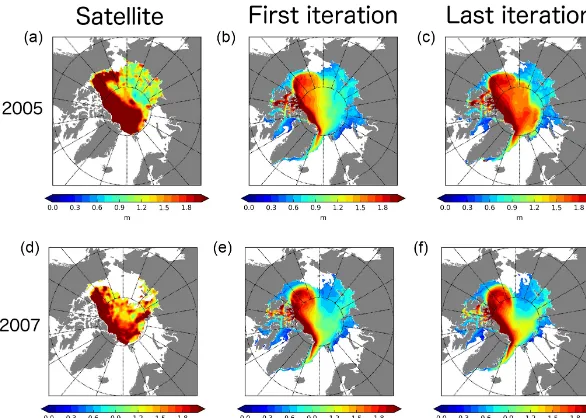
Changes in SIT as a result of SIC assimilation and compar-isons of the former with satellite data are shown in Fig. 9. The satellite ice thickness data are obtained from ICESat campaigns (Kwok et al., 2007), distributed on a 25 km grid and available from the NASA Jet Propulsion Laboratory (http://rkwok.jpl.nasa.gov/icesat/index.html). ICESat sea ice thickness estimates are considerably larger than those in the simulations, especially in the Canadian sector of the Arctic Ocean. One should note that the uncertainty for this observa-tional data is quite large (just better than 0.7 m; Kwok et al., 2007), while the spatial distribution of the thickness is prob-ably realistic (Kwok and Cunningham, 2008).
The ice in October–November 2005 became thicker in the Eurasian Basin of the Arctic Ocean after assimilation and in general became closer to the observed thickness distribu-tion. The thickness increase is considerable, reaching 0.5 m in some places. The shape of the region with the largest thick-ness increase in the Eurasian Basin resembles the shape of the September SIC distribution (Fig. 3) and because of its similarity in pattern it is probably a result of the control vari-able’s corrections that aim to thermodynamically increase SIC in this region. Results for October–November 2007 are similar, with improved thickness along the continental shelf of the Eurasian Basin. However, thickness increase is not as strong as for 2005, reaching only about 0.3 m. A general ten-dency of these improvements is an increase in thickness in the central Arctic and the Canadian Basin, while regions with thin ice over the shelf seas tend to decrease in thickness. This tendency was also shown by (Fenty et al., 2015) for the year 2004.
Figure 9.Sea ice thickness in October–November for years 2005(a–c)and 2007(d–f). Panels(a, d)present satellite data (ICESat, Kwok data);(b, e)are model results before assimilation (first iteration);(c, f)correspond to model results after assimilation (last iteration).
5.2 Ocean changes
Local changes of the SIC are caused by corrected atmo-spheric conditions (see above), which in the coupled sys-tem will also affect near-surface ocean parameters. To some extent changes can also come about through change in the ocean circulation, and we therefore want to investigate how large those changes are and to what extent they could con-tribute to the sea ice improvements.
Figure 10 shows differences in temperature and salinity between the initial and final iterations of the assimilation sys-tem for June and Sepsys-tember of year 2005. The month of June is chosen because corrections to thermodynamic control vari-ables during this month are largest (see above in Sect. 4). The sea surface temperature differences are mostly positive along the ice edge, where the model produces too much ice in the initial iteration (Fig. 3), and lower in magnitude in the central part of the Arctic Ocean. In June, considerable tem-perature differences cover a much smaller area compared to September, since most of the shelf seas are still covered by high concentrations of sea ice and most of the additional en-ergy resulting from the correction to thermodynamic control variables is spent directly in the sea ice melting.
The surface salinity (Fig. 10, right column) shows an in-crease in the Eurasian Basin, caused by additional sea ice production (or less melting). There is a decrease of salinity around the sea ice edge due to melting of excessive sea ice formed in the initial iteration. In September, however, there is a pronounced increase in salinity in most of the Arctic shelf seas. This might be a result of the local increase in sea ice production in areas which become free of ice due to the sum-mer corrections (e.g., Laptev Sea) but still have quite
nega-tive temperatures in the original forcing that are not corrected in September (corrections in September are quite small) at the onset of the freezing period.
Due to the relatively short assimilation periods (1 year) and to the extremely low amount of vertical temperature– salinity profile observations, improvements in the vertical distribution of temperature and salinity after 9 years of as-similation are quite small. Nevertheless, the positive bias in the Atlantic water layer temperature of the Eurasian Basin, which is characteristic for the forward run, has been slightly reduced (not shown). In contrast, changes in the upper part of the water column due to sea ice corrections, although hardly penetrating deeper than the first 50 m, may influence integral fluxes at the borders of the Arctic Ocean.
We have calculated volume, heat and freshwater fluxes (Table 2) through the main passages of the Arctic Ocean (ex-cept for Bering Strait, where fluxes are largely prescribed in the model by the boundary conditions). Along with the initial and final iterations, results for a no-assimilation for-ward simulation were analyzed in order to remove the effect of changing the initial conditions at the beginning of each assimilation year. These may lead to changes of long-term variability and may affect the fluxes towards the end of the assimilation period. We also show mean fluxes for August-September of year 2005 and compare them to the results of Tsubouchi et al. (2012), who applied an inverse model to data obtained in summer 2005 to calculate net fluxes of volume, heat and freshwater around the Arctic Ocean boundary.
Figure 10.Differences in ocean surface temperature(a, c)and salinity(b, d)between the first-guess and last iteration for June 2005(a, b) and September 2005(c, d).
Table 2.Mean values of different fluxes through Arctic Ocean passages.
Parameter Forward After Difference Forward After assimilation Tsubouchi et
and passage assimilation in % 2005 2005 al. (2015)
Volume flux (Sv)
Fram Strait −3.12 −3.12 −0.02 −4.0 −4.49 −1.6±3.9
Davis Strait −0.50 −0.55 4.72 0.44 0.03 −3.1±0.7
Barents Sea Opening 2.78 2.81 0.88 3.5 3.6 3.6±1.1
St. Anna Trough −2.01 −2.01 0.18
Heat flux (TW)
Fram Strait 38.76 38.62 −0.36 41.5 39.9 62±17
Davis Strait 7.94 7.69 −3.12 8.6 6.3 28±3
Barents Sea Opening 83.10 84.07 1.17 111.8 115.8 86±19
St. Anna Trough 1.02 0.20 −80.13
Freshwater flux (mSv)
Fram Strait −113.50 −109.80 −3.20 −173.0 −141.0 −70.0±40
Davis Strait −25.60 −27.27 6.50 13.5 −11.3 −119±14
Barents Sea Opening −21.81 −22.37 2.57 −22.5 −22.0 −31±13
Figure 11.Fluxes through the Fram and Davis straits of(a) vol-ume,(b)heat and(c)freshwater. Positive fluxes are into the Arctic Ocean. Results are shown for the forward run (red), for the run be-fore assimilation (blue) and for the run after assimilation (green).
above do not contribute considerably to changes in the ocean circulation. This is expected since the amount of sea ice con-centration data is much larger than the number of hydro-graphic observations in the Arctic Ocean, so that the assim-ilation system tries to change control variables in a way that will have larger impact on the sea ice. However, episodically, significant changes can be observed (for example in summer 2008) when modifications in the throughflows across Fram Strait are noticed, which are about 60 % larger than in the forward simulation without data assimilation (Fig. 11a).
Differences in the heat flux (Fig. 11b) at Fram and Davis straits can be episodically relatively large, but they do not show any particular tendency and may be related to the lo-cal heating or cooling in the vicinity of the sections. Table 2 summarizes the mean differences for the analyzed passages and, although hardly visible in the time series (not shown),
heat flux differences for the St. Anna Trough are the largest on average, reducing the heat export from the Arctic Ocean by about 80 %.
The freshwater flux differences (Fig. 11c) are most visible in the Fram Strait time series, but positive and negative dif-ferences remain comparable to the forward run and compen-sate each other, such that on average the relative difference is only about 3 %. Large relative differences again occur for the St. Anna Trough (Table 2), which is located in an area with strong atmospheric corrections during most of the years.
Considering Tsubouchi et al. (2012) to be a good approx-imation of observed values in August–September 2005, it is hard to definitely conclude if ocean fluxes become better or worse after the assimilation (Table 2). Some values, such as the volume flux through Davis Strait and the Barents Sea Opening or the freshwater flux in the Fram and Davis straits, have changed and became closer to the values of Tsubouchi et al. (2012). Other values moved even further away from their estimates.
From the combined analysis of Fig. 11 and Table 2 one can conclude that, while on average most of the transports are hardly affected by the assimilation, during some periods relative large differences between the simulations with as-similation and the forward run without asas-similation can be seen and may reach 60–100 % for major straits.
6 Concluding remarks
Results from a multi-year data assimilation attempt based on a coupled Arctic Ocean–sea ice system were presented. The largest improvements relative to simulations without data as-similation were seen for the SIC and SST. Most of the im-provements in the SIC happened during summer months and manifest themselves in a more realistic position of the sea ice edge and in SIC values closer to observations in the central Arctic.
the corresponding transports in simulations without assimi-lation. The latter can still be important for local process stud-ies or model validation against observations that are limited in time.
With the use of the adjoint assimilation technique, we pro-duced a model simulation that is considerably closer to ob-servations and at the same time dynamically consistent. This data can be used for further understanding of the reasons and consequences of changes in the Arctic Ocean.
Data availability. The MITgcm model is free, open source, and can be downloaded from http://mitgcm.org/. For this research version c63m is used. The data produced by the data assimilation system are available from the corresponding author upon request. Sources of assimilated data are listed in the Table 1.
Competing interests. The authors declare that they have no conflict of interest.
Acknowledgements. This work was funded in part by the Euro-pean Union 7th framework program through the MONARCH-A Collaborative Project, FP7-Space-2009-1 contract no. 242446. Nikolay V. Koldunov is also supported by the project S1 (“Climate models as metrics”) of the Collaborative Research Centre TRR 181 “Energy Transfer in Atmosphere and Ocean” funded by the German Research Foundation (DFG). The model integrations were performed at the Deutsches Klimarechenzentrum (DKRZ), Hamburg, Germany. We thank two anonymous reviewers for their constructive comments, which helped to improve the manuscript.
The article processing charges for this open-access publication were covered by the University of Bremen.
Edited by: Christian Haas
Reviewed by: three anonymous referees
Comiso, J. C., Parkinson, C. L., Gersten, R., and Stock, L.: Acceler-ated decline in the Arctic sea ice cover, Geophys. Res. Lett., 35, L01703, https://doi.org/10.1029/2007GL031972, 2008. Dukhovskoy, D. S., Ubnoske, J., Blanchard-Wrigglesworth, E.,
Hi-ester, H. R., and Proshutinsky, A.: Skill metrics for evaluation and comparison of sea ice models, J. Geophys. Res.-Oceans, 120, 5910–5931, https://doi.org/10.1002/2015JC010989, 2015. ESA SICCI: ESA SICCI project consortium: D2.6: Algorithm
The-oretical Basis Document (ATBDv1), ESA Sea Ice Climate Ini-tiative Phase 1, Tech. Rep. SICCI-ATBDv1-04-13, ESA, Paris, France, 2013.
Fekete, B., Vorosmarty, C., and Grabs, N.: Global, composite runoff fields based on observed river discharge and simulated water bal-ances, Technical Report, Global Runoff Data Center, Koblenz, Germany, 1999.
Fenty, I. and Heimbach, P.: Coupled Sea Ice–Ocean-State Estima-tion in the Labrador Sea and Baffin Bay, J. Phys. Oceanogr., 43, 884–904, https://doi.org/10.1175/JPO-D-12-065.1, 2013a. Fenty, I. and Heimbach, P.: Hydrographic Preconditioning for
Sea-sonal Sea Ice Anomalies in the Labrador Sea, J. Phys. Oceanogr., 43, 863–883, https://doi.org/10.1175/JPO-D-12-064.1, 2013b. Fenty, I., Menemenlis, D., and Zhang, H.: Global coupled
sea ice-ocean state estimation, Clim. Dynam., 49, 931–956, https://doi.org/10.1007/s00382-015-2796-6, 2015.
Giering, R. and Kaminski, T.: Recipes for adjoint code construction, ACM T. Math. Softw., 24, 437–474, https://doi.org/10.1145/293686.293695, 1998.
Giering, R., Kaminski, T., and Slawig, T.: Generating efficient derivative code with TAF adjoint and tangent linear Euler flow around an airfoil, Future Gener. Comp. Sy., 21, 1345–1355, https://doi.org/10.1016/j.future.2004.11.003, 2005.
Hibler, W. D.: Dynamic thermodynamic sea ice model, J. Phys. Oceanogr., 9, 815–846, https://doi.org/10.1175/1520-0485(1979)009, 1979.
Hibler, W. D.: Modeling a variable thickness sea ice cover, Mon. Weather Rev., 108, 1943–1973, 1980.
Hibler, W. D.: The role of sea ice dynamics in modeling CO2 in-creases, in: Climate processes and climate sensitivity, edited by: Hansen, J. E. and Takahashi, T., Vol. 29 of Geophysical Mono-graph, 238–253, AGU, Washington, D.C., 1984.
Jahn, A., Aksenov, Y., Cuevas, B., Steur, L., Häkkinen, S., Hansen, E., Herbaut, C., Houssais, M.-N., Karcher, M., Kauker, F., and Lique, C.: Arctic Ocean freshwater: How robust are model simulations?, J. Geophys. Res.-Oceans, 117, C00D16, https://doi.org/10.1029/2012JC007907, 2012.
Jakobson, E., Vihma, T., Palo, T., Jakobson, L., Keernik, H., and Jaagus, J.: Validation of atmospheric reanalyses over the central Arctic Ocean, Geophys. Res. Lett., 39, L10802, https://doi.org/10.1029/2012GL051591, 2012.
Kalnay, E., Kanamitsu, M., Kistler, R., Collins, W., Deaven, D., Gandin, L., Iredell, M., Saha, S., White, G., Woollen, J., Zhu, Y., Leetmaa, A., Reynolds, B., Chelliah, M., Ebisuzaki, W., Higgins, W., Janowiak, J., Mo, K. C., Ropelewski, C., Wang, J., Jenne, R., and Joseph, D.: The NCEP/NCAR 40-year reanalysis project, B. Am. Meteorol. Soc., 77, 437–471, 1996.
Kauker, F., Kaminski, T., Karcher, M., Giering, R., Gerdes, R., and Voßbeck, M.: Adjoint analysis of the 2007 all time Arctic sea-ice minimum, Geophys. Res. Lett., 36, L03707, https://doi.org/10.1029/2008GL036323, 2009.
Knudsen, P. and Andersen, O. B.: A Global Mean Ocean Circulation Estimation Using GOCE Gravity Models – The DTU12MDT Mean Dynamic Topography Model, in: 20 Years of Progress in Radar Altimetry, ESA publications (ESA SP-710), Venice, Italy, 2013.
Knudsen, P., Bingham, R., Andersen, O., and Rio, M.-H.: A global mean dynamic topography and ocean circulation estimation us-ing a preliminary GOCE gravity model, J. Geodesy, 85, 861–879, https://doi.org/10.1007/s00190-011-0485-8, 2011.
Köhl, A.: Evaluation of the GECCO2 ocean synthesis: transports of volume, heat and freshwater in the Atlantic, Q. J. Roy. Meteor. Soc., 141, 166–181, https://doi.org/10.1002/qj.2347, 2015. Köhl, A. and Stammer, D.: Variability of the meridional
over-turning in the North Atlantic from the 50-year GECCO state estimation, J. Phys. Oceanogr., 38, 1913–1930, https://doi.org/10.1175/2008JPO3775.1, 2008.
Köhl, A. and Willebrand, J.: An adjoint method for the assim-ilation of statistical characteristics into eddy-resolving ocean models, Tellus A, 54, 406–425, https://doi.org/10.1034/j.1600-0870.2002.01294.x, 2002.
Koldunov, N. V., Köhl, A., and Stammer, D.: Properties of adjoint sea ice sensitivities to atmospheric forcing and implications for the causes of the long term trend of Arctic sea ice, Clim. Dynam., 41, 227–241, https://doi.org/10.1007/s00382-013-1816-7, 2013. Koldunov, N. V., Serra, N., Köhl, A., Stammer, D., Henry, O., Cazenave, A., Prandi, P., Knudsen, P., Andersen, O. B., Gao, Y., and Johannessen, J.: Multimodel simulations of Arctic Ocean sea surface height variability in the pe-riod 1970–2009, J. Geophys. Res.-Oceans, 119, 8936–8954, https://doi.org/10.1002/2014JC010170, 2014.
Krishfield, R., Toole, J., Proshutinsky, A., and Timmermans, M.-L.: Automated ice-tethered profilers for seawater observations under pack ice in all seasons, J. Atmos. Ocean. Tech., 25, 2091–2105, 2008.
Kwok, R. and Cunningham, G.: ICESat over Arctic sea ice: Esti-mation of snow depth and ice thickness, Journal of Geophysical Research: Oceans, 113, 2008.
Kwok, R. and Rothrock, D. A.: Decline in Arctic sea ice thickness from submarine and ICESat records: 1958–2008, Geophys. Res. Lett., 36, L15501, https://doi.org/10.1029/2009GL039035, 2009.
Kwok, R., Cunningham, G. F., Zwally, H. J., and Yi, D.: Ice, cloud, and land elevation satellite (ICESat) over Arctic sea ice: Retrieval of freeboard, J. Geophys. Res., 112, C12013, https://doi.org/10.1029/2006JC003978, 2007.
Large, W. G., McWilliams, J. C., and Doney, S. C.: Oceanic vertical mixing: A review and a model with a nonlocal boundary layer parameterization, Rev. Geophys., 32, 363–403, https://doi.org/10.1029/94rg01872, 1994.
Lee, C., Melling, H., Eicken, H., Schlosser, P., Gascard, J.-C., Proshutinsky, A., Fahrbach, E., Mauritzen, C., Morison, J., and Polykov, I.: Autonomous platforms in the arctic observing net-work, Proceedings of Ocean Obs09: Sustained Ocean Observa-tions and Information for Society, 2, ESA Publication WPP-306, Venice, Italy, 2010.
Lindsay, R. W. and Zhang, J.: Assimilation of ice concentration in an ice-ocean model, J. Atmos. Ocean. Tech., 23, 742–749, https://doi.org/10.1175/JTECH1871.1, 2006.
Lisæter, K. A., Rosanova, J., and Evensen, G.: Assimilation of ice concentration in a coupled ice–ocean model, using the Ensemble Kalman filter, Ocean Dynam., 53, 368–388, https://doi.org/10.1007/s10236-003-0049-4, 2003.
Liu, C., Köhl, A., and Stammer, D.: Adjoint-based estimation of eddy-induced tracer mixing parameters in the global ocean, J. Phys. Oceanogr., 42, 1186–1206, 2012.
Losch, M., Menemenlis, D., Campin, J.-M., Heimbach, P., and Hill, C.: On the formulation of sea-ice mod-els. Part 1: Effects of different solver implementations and parameterizations, Ocean Model., 33, 129–144, https://doi.org/10.1016/j.ocemod.2009.12.008, 2010.
Marshall, J., Adcroft, A., Hill, C., Perelman, L., and Heisey, C.: A finite-volume, incompressible Navier Stokes model for studies of the ocean on parallel computers, J. Geophys. Res.-Oceans, 102, 5753–5766, https://doi.org/10.1029/96JC02775, 1997.
Nguyen, A. T., Menemenlis, D., and Kwok, R.: Arctic ice-ocean simulation with optimized model parameters: Approach and assessment, Journal of Geophysical Research, 116, C04 025+, https://doi.org/10.1029/2010JC006573, 2011.
Nilsen, J. E. O., Hátún, H., Mork, K. A., and Valdimarsson, H.: The NISE Dataset, Technical Report, Faroese Fisheries Laboratory, Tórshavn, Faroe Islands, 2008.
OSI-SAF: EUMETSAT Ocean and Sea Ice Satellite Applica-tion Facility. Global sea ice concentraApplica-tion reprocessing dataset 1978–2015 (v1.2), available at: http://osisaf.met.no/, last access: September 2015.
Overland, J. E. and Wang, M.: When will the summer Arctic be nearly sea ice free?, Geophys. Res. Lett., 40, 2097–2101, https://doi.org/10.1002/grl.50316, 2013.
Proshutinsky, A., Aksenov, Y., Clement Kinney, J., Gerdes, R., Gol-ubeva, E., Holland, D., Holloway, G., Jahn, A., Johnson, M., Popova, E., Steele, M., and Watanabe, E.: Recent Advances in Arctic Ocean Studies Employing Models from the Arctic Ocean Model Intercomparison Project, Oceanography, 24, 102–113, https://doi.org/10.5670/oceanog.2011.61, 2011.
Remote Sensing System database: Remote Sensing Systems, http: //www.remss.com/, last access: September 2014.
Boschung, J., Nauels, A., Xia, Y., Bex, V., and Midgley, P. M.: Climate change 2013: The physical science basis, IPCC, 2014. Tietsche, S., Notz, D., Jungclaus, J. H., and Marotzke, J.:
As-similation of sea-ice concentration in a global climate model – physical and statistical aspects, Ocean Sci., 9, 19–36, https://doi.org/10.5194/os-9-19-2013, 2013.