A Novel Technique for Solving Multiobjective Fuzzy Linear Programming Problems

Abstract–This study considers multiobjective fuzzy linear

programming (MFLP) problems in which the coefficients in the

objective functions are triangular fuzzy numbers. The study proposing a new technique to transform MFLP problems into the equivalent single fuzzy linear programming problem and then solving it via linear ranking function using the simplex method, supported by numerical example.

Index Terms—Triangular fuzzy numbers, Multiobjective fuzzy linear programming problems, Linear ranking function, Compromise solution.

I. Introduction

A basic linear programming (LP) problem deals only with a single linear objective function subject to a linear constraint set, and the assumption that parameters are known with certainty. LP problems involving more than

one possibly conflicting objective functions are called

multiobjective linear programming (MLP) problems. Multiobjective fuzzy linear programming (MFLP)

problems occur when the objective functions coefficients

are fuzzy numbers (FNs).

Tanaka, et al. (1974a) first introduced fuzzy linear

programming (FLP) problems, building on fuzzy environment presented by Bellman and Zadeh (1970). Zimmermann (1978) introduced the formulation of FLP problem and constructed a model of the problem also based on the fuzzy concepts of Bellman and Zadeh (1970). By the beginning of the current century, FLP problems have been used in broadly different real life problems (Iskander, 2002; Zhang, et al., 2005; Rong and Lahdelma, 2008; Chen and Ko, 2009; Peidro, et al., 2010; Hassanzadeh, et al., 2011).

Ebrahimnejad and Tavana (2014) classified FLP problems into five main groups based on findings of various researchers

(Zimmermann, 1987; Luhandjula, 1989; Inuiguchi, et al., 1990; Buckley and Feuring, 2000; Hashemi, et al.,

2006; Dehghan, et al., 2006; Allahviranloo, et al., 2008;

Hosseinzadeh Lotfi, et al., 2009; Kumar, et al., 2011). In a fully fuzzified LP problem where all the parameters

and variables are FNs, Buckley, and Feuring (2000) changed the problem of maximizing an FN, the objective function’s value into an MFLP problems. They proved that all undominated set to MFLP problems can be explored by

fuzzy flexible programming.

An interactive fuzzy programming was proposed by Sakawa, et al. (2000) to solve MLP problems with fuzzy parameters. After defuzzifying the fuzzy goals of the decision

makers (DMs), a satisfactory solution is derived efficiently by

updating the satisfactory degrees of the DMs at the topmost levels with respectfulness stable satisfactory among all levels.

MFLP vector optimization problems of a fuzzy nature were considered by Cadenas and Verdegay (2000) who assumed that all the objective functions involved come from

the same DM with FN coefficients and they can be defined

by different DMs.

Stanciulescu, et al. (2003) formulated a multiobjective

decision-making process in which the coefficients of the

objective functions and the constraints are fuzzy as MFLP problems. Their method uses fuzzy decision variables with a joint membership function instead of crisp decision variables. The lower bound fuzzy decision variables set up the lower bounds of the decision variables and generalize to lower-upper bound fuzzy decision variables that in turn set up the upper bounds of the decision variables too. The Optimal solutions (OSs) of the problem and their method supply to the DM regions containing potential satisfactory solutions around the OSs.

Cadenas and Verdegay (2000) used a ranking function in dealing with MFLP problems, multiobjective mathematical programming problems, vector optimization programming (VOP) problems, and Fuzzy Multiobjective Optimization problems. Ganesan and Veeramani (2006) introduced FLP with symmetric trapezoidal fuzzy numbers and proposed to solve this kind of problems using ranking function for FNs, without converting the problem to crisp LP problem. In the study of MFLP model for supplier selection in supply chain (Amid, et al., 2006), an MFLP model was developed with vagueness, imprecision of the goals, constraints, and parameters in which

the decision-making has been made difficult for such kind of

problems (Mahdavi-Amiri and Nasseri, 2006).

A Novel Technique for Solving Multiobjective Fuzzy

Linear Programming Problems

Abdulqader O. Hamadameen

Department of Mathematics, Faculty of Science and Health, Koya University, Danielle Mitterrand Boulevard, Koya KOY45, Kurdistan Region - F.R. Iraq

ARO-The Scientific Journal of Koya University Volume V, No 1(2017), Article ID: ARO.10064, 8 pages DOI: 10.14500/aro.10064

Received 11 January 2015; Accepted 13 September 2015 Regular research paper: Published 31 March 2017

Wu (2008a) derived the optimality conditions for LP

problems with fuzzy coefficients when considering the

orderings of the set of all FNs and proposed two solution approaches. Nondominated solution was proposed in the MLP problem by naturally eliciting the optimality conditions. To solve MFLP problems, Wu (2008b) converted the problem into a VOP problem by employing the embedding proposition

and using appropriate linear defuzzification functions.

In some MFLP models, both the objective functions and

the constraints are fuzzy. Furthermore, the coefficients of the

decision variables in the objective functions, constraints, and the right-hand sides of the constraints are assumed to be FNs with either triangular or trapezoidal membership functions. Iskander (2008) proposed to utilize possibilistic programming to transform such MFLP problems as previously modeled (Negi and Lee, 1993) into its equivalent crisp programming

according to the author’s modifications. Iskander (2002,

2008) used two main criteria with the same evaluation concept in MFLP: The global criterion method and the distance functions method.

Baky (2009) proposed fuzzy goal programming algorithm for solving decentralized MFLP problems in the form of bilevel programming problems to obtaining OS for the problem. In another paper, the researcher (Baky, 2010) presented two new algorithms to solve MFLP problems through the fuzzy goal programming approach.

Amid, et al. (2011) developed a weighted max–min method and used it to solve MFLP problems to help managers of supplier selection and allow them to assign the order quantities to each supplier based on supply chain strategies.

Gupta and Kumar (2012) studied Chiang’s method (Chiang, 2005) and pointed out the shortcomings in the latter’s method. Hence, they proposed a new method to overcome these weaknesses of the MFLP problems by

representing all the parameters in the system as (λ, ρ)

interval-valued FNs.

In their review paper, Hamadameen and Zainuddin (2013) focused on various kinds of MFLP problems. They discussed the main studies in the recent years comprehensively. They considered problems with fuzziness in both the objective functions and constraints and analyzed MFLP problems chronologically. They also described problem formulation and the various research methodologies in MFLP problems. In addition, they surveyed many transformation methods that have been used to convert MFLP problems into their corresponding equivalent deterministic MLP problems. Moreover, they also addressed OSs for the original problem in each study.

Luhandjula and Rangoaga (2014) presented a new approach in solving continuous optimization problems based on the nearest interval approximation operator for dealing with an MFLP problem. They established a Karush-Kuhn-Tucker (KKT) kind of pareto optimality conditions. There

were two crucial algorithms in the proposed method; the first

gave nearest interval approximation to a given FN, and the second provided KKT conditions to deliver a pareto OS.

In this study, we address the MFLP problems in which

objective functions’ coefficients are triangular fuzzy numbers

(T_rFNs). The study utilizes a linear ranking function through simplex method, in addition a new method to transform

the MFLP problems into single FLP problem and find a

compromise solution for the original problem, in which consists in minimizing the sum of distances from the

objective functions to predefined ideal values. This paper is organized as follows: Section 2 defines fuzzy concepts

and algebra properties of T_rFNs. Section 3 addresses linear ranking functions and the comparison of FNs. In addition, it gives the mathematical formulation of the T_rFNs. Section 4

defines the mathematical formulation for FLP problem and

MFLP problems. Section 5 addresses OS, simplex method, and compromise solution for MFLP problems. Solution algorithms are presented in Section 6. In Section 7, to illustrate the proposed method, a numerical example is solved. Conclusions are discussed in Section 8.

II. Preliminaries of Fuzzy Concepts

This study uses some of the concepts of fuzzy sets. We list

here some definitions and properties.

A. Basic Definitions

Fuzzy set: Let X be the universal set. à is called a fuzzy set in X if à is a set of ordered pairs à = {(x,μ_à (x))x ∈ X}; where μ_à (x) is the membership function of x ∈ à (Sakawa, 1993). Note that the membership function of à is a characteristic (indicator) function for à and it shows to what degree x∈ Ã.

α-level set: The α-level set of à is the set Ã_α={x∈R|μ_Ã(x)≥α}, where α ∈ [0,1]. The lower and upper bounds of α-level set à are finite numbers represented by inf

x ∈ Ã_α and sup x ∈ Ã_α, respectively (Wang, 1997; Sakawa, 1993; Yager and Filev, 1994).

Normal Fuzzy Set: The height of a fuzzy set is the largest membership value attained by any point. If the height of fuzzy set equals one, it is called a normal fuzzy set (Wang, 1997).

The core (modal): The core of a fuzzy set à of X is the crisp subset of X consisting of all elements with membership grade one, or core (Ã)=

{

x|Ã(x) = 1 and x ∈X

}

(Yager and File, 199).

The support: The support of a fuzzy set à is a set of elements in X for which Ã(x) is positive, that is, supp Ã={x∈X|µ_Ã(x)>0} (Wang, 1997; Sakawa, 1993).

Fuzzy convex set: A fuzzy set à is convex if

(

)

(

1

)

{

( )

,

( )

}, , [0,1]

A x y min A A x y x y X

  + − ≥   ∀ ∈ ∧∈

(Wang, 1997; Sakawa, 1993).

Convexity and fuzzy number (FN): A convex fuzzy set à on  is an FN if: one its membership function is piecewise continuous; two there exist three intervals [a, b], [b, c] and [c, d] such that à is increasing on [a, b], equal to 1 on [b

,

c]

,

decreasing on [c

,

d]

,

and equal to

₀

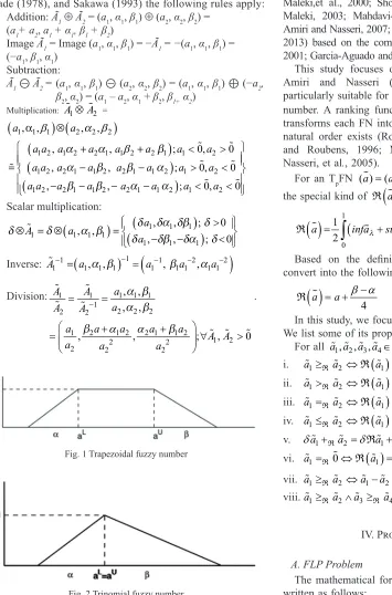
elsewhere ∀ a b c, ,  ∈ (Mahdavi-Amiri and Nasseri, 2006; Mahdavi-Amiri and Nasseri, 2007).

The trapezoidal fuzzy number (T_pFN): Let à = (aL_{, a}U_,

[aL _{− α, a}U _{+ β] its support part (Mahdavi-Amiri and Nasseri,} 2006; Mahdavi-Amiri and Nasseri, 2007) (Fig. 1).

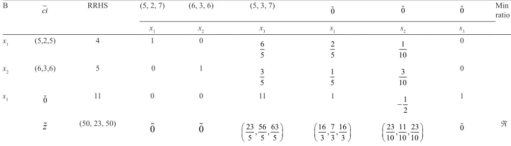
If a = aL _{= a}U _{∈ Ã then the T}

pFN is reduced to TrFN and

denoted by à = (a, α, β) (Fig. 2). Thus, à = (a, α, β) ⊂ (aL_{, a}U_{, α, β). Since the study is focused on MFLP problems} with T_rFNs, the next section lists algebra properties specific

to such FNs.

B. Algebra Properties of FNs

Let Ã₁, Ã₂ ∈ TrFNs, such that Ã₁ = (a₁, α₁, β₁) and Ã₂= (a₂, α₂, β₂), then based on Zadeh (1965), Dubois and Prade (1978), and Sakawa (1993) the following rules apply: 1. Addition: Ã₁ ⊕ Ã₂ = (a₁, α₁, β₁) ⊕ (a₂, α₂, β₂) =

(a₁+ a₂, a₁ + α₁, β₁ + β₂)

2. Image Ã₁ = Image (a₁, α₁, β₁) = −Ã₁ = −(a₁, α₁, β₁) =

(−a₁, β₁, α₁) 3. Subtraction:

Ã₁⊝ Ã₂ = (a₁, α₁, β₁) ⊝ (a₂, α₂, β₂) = (a₁, α₁, β₁) ⊕ (−a₂,

β₂, α₂) = (a₁ – a₂, α₁ + β₂, β₁₊ α₂)

4. Multiplication: A A₁⊗ ₂ =

(

) (

)

(

)

(

)

(

)

1 1 1 2 2 2

1 2 1 2 2 1 1 2 2 1 1 2

1 2 2 1 1 2 2 1 1 2 1 2

1 2 2 1 1 2 2 1 1 2 1 2

, , ,

, , ; 0, 0

, , ; 0, 0

, , ; 0, 0

a a

a a a a a a a a

a a a a a a a a

a a a a a a a a



  

   

   

α ⊗

+ +

= − −

− − − −

,



 

 





β β

β

 < > 

 

 _{> <} 

 

 _{< <} 

 

 

5. Scalar multiplication:

(

)

(

(

1 1 1

)

)

1 1 1 1

1 1 1

, , ; 0

, ,

, , ; 0

a

A a

a

   

   

   

⊗ = ⊗ =

− −

 _ > _

<

 

 

6. Inverse: 1

(

)

1

(

1 2 2

)

1 1, ,1 1 1 , 1 1 , 1 1

A− = a   − ₌ a a−  −  a−

7. Division: 1 1 1 1 1 1

2 2 2

2 2

1 2 1 2 2 1 1 2

1 2

2 2

2 2 2

, , , ,

, , ; , 0

A A a

a

A A

a a a a a _{A A}

a a a

   

 

 

 

  

α α

−

= =

 + + 

=_ _ ∀ >

 

.

Note that similar formulas hold when A1<0 ,A2 >0 or

   

A1>0,A2 <0

8. A1= ⇔0 A1=

(

0 0 0, ,

)

.

III. Ranking Functions and the Comparison of FN The first step in solving MFLP is to defuzzify the fuzzy

assertion. One of the several tools used to achieve this aim is a ranking function (Fang and Hu, 1996; Lai and Hwaang, 1992; Maleki,et al., 2000; Shoacheng, 1994; Tanaka, et al., 1974b; Maleki, 2003; Amiri and Nasseri, 2006; Mahdavi-Amiri and Nasseri, 2007; Ebrahimnejad, 2011; Ullah Khan,et al., 2013) based on the comparison of the FNs (Wang and Kerre, 2001; Garcia-Aguado and Verdegay, 1993; Maleki, 2003).

This study focuses on a ranking function by Mahdavi-Amiri and Nasseri (2007). This ranking function is particularly suitable for T_pFNs. It transforms the FN to a real number. A ranking function R:F R

( )

→is a map which

transforms each FN into its corresponding real line, where a

natural order exists (Roubens and Jacques, 1991; Fortemps

and Roubens, 1996; Mahdavi-Amiri and Nasseri, 2007; Nasseri, et al., 2005).

For an T_pFN ( )_a  ₌( ,_{a a} L U, ,_{ ), Yager (1981) proposed}

the special kind of R

( )

a� formulated as follows:



( )

1

(

)

0 1

2 2 4

L U

a a

a =

∫

infa+supa d = + + β−

R (1)

Based on the definition of TrFN, and TpFN, (1) can

convert into the following form for the TrFNs:



( )

a a= +β α₄−

R (2)

In this study, we focus only on the linear ranking function. We list some of its properties on FNs.

For all a a a a   1, 2, 3, 4∈�FNs, and δ∈ then:

i. a1≥R a2 ⇔R

( )

a1 ≥R

( )

a2

ii. a1>Ra2⇔R

( )

a1 >R a

( )

2

iii. a1=Ra2⇔R

( )

a1 =R

( )

a2

iv. a1≤R a2 ⇔R

( )

a1 ≤R

( )

a2

v. δa1+Ra2 =δRa1+R

( )

a2

vi. a1=R0⇔R

( )

a1 =R

( )

0 =0

vii. a1≥R a2 ⇔a a1−2 ≥R 0⇔ − ≥ −a2 R a1

viii. a1≥R a2∧a3≥Ra4� ⇔a a1+ 3≥R a2+a�4

IV. Problem Formulation

A. FLP Problem

The mathematical formulation of the FLP problem can be written as follows:

Fig. 1 Trapezoidal fuzzy number

( )

. . 0

Max z x cx

s t Ax b x



 =

≤ ≥

R

(3)

Where _cT_{, A and b are of dimentions (n, 1), (m, n) and}

(m, 1), respectively. A feasible solution for (3) is the vector x∈Rn _{which satisfies the constraints and their signs. In} addition, x

*

is an optimal feasible solution for (3) if and only if _cx* _{≥ cx } ,

R for all feasible solution x. On the other side of the constraints of (3), if Rank (A, b) = Rank (A) = m, then after partition and rearranging of the columns of A = [B, N], where the nonsingular matrix B = (m, m), and rank (B) = m where x_B = B−1 _{b, x}

N = 0; then, the basic solution point

(

T, T

)

T B N

x x x is called the basic feasible solution (BFS) for the system in (3), where band nare basic matrix, and non-basic matrix, respectively (Nasseri, et al., 2005).

B. MFLP Problem

The mathematical formulation of the MFLP problems can be written as follows:

( )

( )

1

1

; 1, ,

; 1, ,

. . 0 n

i ij j

j n

ij j j

Max Z x c x i r

Min Z x c x i r s

s t Ax b x

 _

 _

=

=

= = …

= = + …

≤ ≥

∑

∑

R

R i

(4)

Where _{c A b }T, , and _{xare as defined in (3).}

V. Simplex Method and Feasible Solution for FLP Problem

For the FLP problem in (3), after converting it to the standard form:

Maxz x c x c s s t Bx Ns b

x s

B N

B N

B N



( )

=  +

+ =

≥ R . .

, 0

(5)

Since,

(

)

1 1 _, 1 1 _.

B N B N N

x ₊ B Ns− ₌B b z c B N c s cB b − ₊  − ₋ ₌  −

R initially s_{N = 0} thus, 1 _, 1 _.

B B

x ₌B b z − ₌ c B b  −

R We can

express (3) in Table I.

In Table I, we have (Dantzig, 1963; Maleki, et al., 2000; Nasseri, et al., 2005; Mahdavi-Amiri and Nasseri, 2007; Sharma, 2012):

1. The fuzzy objective row, γ_j c B a_{B j} c_{j j B} j

=_R −

≠

−

(

1

)

continuous the γ_j=_R z_j−c_j for the nonbasic variables. 2. For the feasible OS, it should be γ_j= ≥ ∀ ≠_R 0, j B_i. 3. If, γ_k <_R0, k B∀ ≠ _i, then exchange x_Br by x_k. After that

satisfyingγ_k = B a− _k

R 1 .

4. If, γ ≤_{k R}0, then x_k is an unbounded solution for the problem.

5. If an m exist such that zm−cm<R0 and there exist a basic index i in which y_{im > 0}, then a pivoting row p can be found in which the pivoting y_pm yields a feasible tableau corresponding fuzzy objective value.

6. For any feasible solution to FLP problem, there are some columns not in the basic solution in which zm−cm<R0 and yim≤0,i= …1, ,sthen the problem is unbounded.

VI. Compromise Solution

Since many objectives of the system usually conflict with

each other, an improvement of one objective may mean the

sacrifice in another. A compromise solution lets the DMs specify partial preferences among conflicting objectives so

that there will be less alternative solutions. This can mean making adjustments to others.

A. A Compromise Solution for MFLP Problems

Since there may be conflicts among the multiple objectives

in the MFLP problems in (4) under the same set of

constraints, it is difficult to find a solution which satisfies all

of those objective functions. Thus, a compromise solution is most realistic and practical for such kinds of the problems. The decision variable may not be common to all OSs in

the presence of conflicts among objectives. However, the

common set of decision variables between objective functions is necessary to facilitate selection of the best compromise solution. The next section summarized the solution algorithm for the method used in this study.

B. Solution Algorithms

Let us now describe the algorithm step by step:

Step 1: Consider the problem as the mathematical form in (4). Step 2: Convert (4) into the standard form as:

( )

( )

1

1

( ); 1, ,

( ); 1, ,

. .

, 0

n

i ijB j ijN j j

n

i ijB j ijN j j

B N

B N

Max Z x c x c s i r

Min Z x c x c s i r s

s t Bx Ns b x s

 _{ }

 _{ }

=

=

= + = …

= + = + …

+ ≤

≥

∑

∑

R

R

(6) Step 3: Use the tableau notifications in Table I to solve each FLP

problem in the form of (5) by simplex method.

Step 4: Assign vi to the optimum value of the objective function Z i_i; = … …1, , ,r ,s.

Step 5: Convert (6) into its corresponding FLP problem as follows:

TABLE I

The FLP Problem

Objective function

value: z ̃ RHS Basic variable: xB

Nonbasic variable: SN

xB 0 1 B−1b B−1b

z ̃ 1 _{c B b}

B −1 �0 c B N cNB −1 −

( )

1, , 1

1, 1

[ ]

[ ] : 0

. .

, 0

n

ij j i i r j

n

ij j i i r s i j

B N

B N

Max Z x Max c x v

Max c x v v

s t Bx Ns b x s

 _{ }



  

= … =

= + … =

=

− ∀ ≠

+ ≤

≥

∑

∑

R 



(7) Step 6: Find an OS for (7) which will give the compromise

solution for the original problem in the (4).

VII. Numerical Example

Consider the following MFLP problems:

( )

(

)

(

)

(

)

( )

(

)

(

)

(

)

( )

(

)

(

)

( )

(

)

(

)

(

)

1 1 2 3

2 1 2 3

3 1 2 3

4 1 2 3

1 2 3

1 2

5,2,5 6,3,6 5,3,7

4,7,11 5,5,9 3,6,10

5

1,3,2 3,4,1 ,9,7

2

3,4,4 3,4,6 3,4,8

. .3 3 7

2 4

Max Z x x x x

Max Z x x x x

Min Z x x x x

Min Z x x x x

s t x x x

x x

 





= + +

= + +

−

 

= − + − _{+  }

 

= − + − + −

− + ≤

− +

R R

R

R

1 2 3

12

4 3 8 10

0, 1,2,3 j

x x x

x j

≤

− + + ≤

≥ = (8)

Solution: First, we solve each objective function subject to the constraints individually, as:

( )

(

)

(

)

(

)

1 1 2 3

3

1

1 2 3 1

1 2 2

1 2 3 3

5,2,5 6,3,6 5,3,7

0

. .3 3 7

2 4 12

4 3 8 10

, 0, 1,2,3

j j

j j

Max Z x x x x

s

s t x x x s

x x s

x x x s

x x j



 =

= + +

+

− + + =

− + + =

− + + + =

≥ =

∑

R

(9) From Table II, we have

{

(

z c_j− _j

)

}

(

) (

) (

)

{

5,5,2 , 6,6,3 , 5,7,3 ,0,0,0 ;   

}

j 1, ,6

=_R − − − = … .

j = 1.,6

Since,

{ }

{

( )

}

5 , 6 , 6,0,0,0 ,3 3

4 4

j j

γ =  = −_ − − _

 

R

j = 1.,6, thus, x₂ should enter the basic solution, and the leaving variable s₂.

The result is as shown in Table III. From Table III, we have

(

)

{

}

8,8,7 ,0, 5,7,3 ,0,

(

)

3 3 3, , ,0 ;

2 2 4 2

j j

z −c = __− _  −  _ _ _

   

 

R j = 1.,6

Since,

{ }

{

( )

}

9 ,0, 6,0,1 ,0 ,1 11 1, ,6

8 16

j j j

γ = γ = −_ − _ = …

 

R .

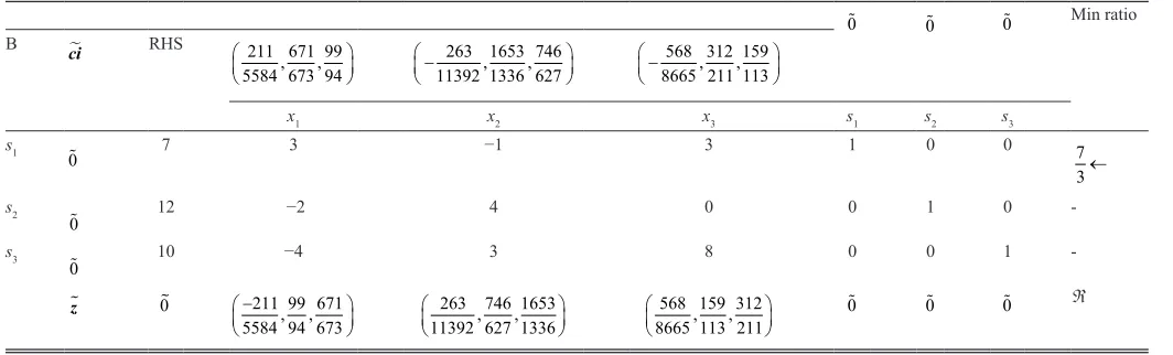
Thus, x₁ should enter the basic solution and the leaving variable s₁. The result is as shown in Table IV.

Now,

(

)

{

}

(

)

23 56 63

0,0, 5,7,3 ,0, , , ,

5 5 5

; 1, ,6

16 7 16_{, , ,} 23 11 23_{, , ,0}

3 3 3 10 10 10

j j

z c j

  

 



 ₋   

   

   

− = _{ } = …

   

 

   

_{   } 

 

R ,

and

{ }

{

( )

}

_0,0,419_{,6 ,2 ,0}1 3 _{0, 1, ,6} 20 12 5

j j j

γ = γ =_ _≥ = …

 

R .

Thus, according to the optimality feasible condition, no more variable can be found to enter the basis, and the OS for the problem (9) is;

(

)

{

z X x x x1; 1 1, ,2 3

}

=

{

(50,23,50) ; (4,5,0)X1

}

.

Using the solution algorithm in Section 6, one can find the

OSs for other z ii; = …2, ,4 as shown in Table V. X_i (x₁, x₂, x₃)

Now, by utilizing (7), the result is a single FLP problem as follows:

TABLE II

The Status of the Solution-1

B _ci RRHS (5,2,5) (6,3,6) (5,3,7) _{0 0 0} Min ratio

x1 x2 x3 s1 s2 s1

s1 0 7 3 −1 3 1 0 0 _

s2 0 12 −2 4 0 0 1 0 3←

s3 0 10 −4 3 8 0 0 1 ₃1

3



z� ₀ (−5,5,2) (−6,6,3) ↑ (−5,7,3) _{0 �0↓ 0} 

Table III

The Status of the Solution-2

B _ci RRHS (5,2,7) (6,3,6) (5,3,7) _{0 0 0} Min

ratio

x1 x2 x3 s1 s2 s1

s1 ₀ 10 3 0 3 1 1

4

0 4←

s2 (6, 3, 6) 3 −2 1 0 0 1

4

0

-s3 0 1 −4 0 8 0 −3

4

1 -

 z�(18 9 18, , )

−    8 8 7_

2 , , ↑ ��0

(-5,7,3) _{0↓ 3}

2 3 4

3 2 , ,

 

( )

{

(

)

(

)

(

)

}

(

)

(

)

(

)

(

)

(

)

(

)

1 2 3

1 2 3

1 2 3

1 2

5,2,5 6,3,6 5,3,7

50,23,50

{ 4,7,11 5,5,9 (3,6,10) } (41,53,89)] 5

1,3,2 3,4,1 ,9,7

2

O 19,32,13

3,4,4 3,4,6

x x x

Max Z x

x x x

x x x

x x  =  + + ⊕    + +  _{− + − +}−       _ _     ₋ ⊕_{ } −   _   − + − + R 

(

)

{

3

}

1 2 3

1 2

1 2 3

3,4,8 ( 28,36,46)]

. .3 3 7

2 4 12

4 3 8 10

0, 1,2,3 j

x

s t x x x

x x

x x x

x j − − − + ≤ − + ≤ − + + ≤ ≥ =

 (10)

This is equivalent to:

( )

1

2 3

1 2 3

1 2

1 2 3

211 671 99_{, ,} 5584 673 94 263 1653 746_{, ,} 568 312 159_{, ,}

11392 1336 627 8665 211 113

. .3 3 7

2 4 12

4 3 8 10

0, 1,2,3 j

Max Z x x

x x

s t x x x

x x

x x x

x j  _{= } _   − −     +_{ } +_{ }     − + ≤ − + ≤ − + + ≤ ≥ = R (11)

The standard form of the above FLP problem is:

( )

1 2

3 3

1

1 2 3 1

1 2 2

1 2 3 3

211 671 99_{, ,} 263 1653 746_{, ,}

5584 673 94 11392 1336 627

568 312 159_{, , 0}

8665 211 113

. .3 3 7

2 4 12

4 3 8 10

0, 1,2,3

j j

j

Max Z x x x

x s

s t x x x s

x x s

x x x s

x j   = −     = _{ } +_{ }     −   +_{ } +   − + + = − + + = − + + + = ≥ =

∑

R (12) Now, using  in (2), through simplex method the solution of the FLP problem (12) is as shown in Table VI.

From Table VII, we have

(

)

{

}

211 99 671_{, , ,} 263 746 1653_{, , ,} 5584 94 673 11392 627 1336

568 159 312_{, , ,0,0,0,} 8665 113 211

1, ,6 j j

z c

j      −             − _{=  }        _{ }    = … R . Since,

{ }

{

( )

}

329 399 719_{, , ,0,0,0 , 1, ,6} 6348 11414 8616

j j j

γ = γ = −_ _ = …

 

R

thus, x₁ should enter the basic solution and the leaving variable is s₁. The result is as shown in Table VII.

In Table VII, since

(

)

{

}

81 396 9661 161 351 1033

0, , , , , ,

7721 257 6155 1558 146 408 61 _, 671 33_{, ,0,0; 1, ,6} 4843 2019 94

j j

, z c

j                        − _{=  }    _{= …}     _{ }    R and

{ }

{

( )

}

_0,106 961_{, ,} 511 _{,0,0 0, 1, ,6.} 5995 7104 29579

j j j

 =  = ≥ = …

 

R

Thus, according to the optimality feasible condition, no more variable may enter the basis, and the OS for the problem (12) is

(

)

{

Z X x x x; 1 2, , 3

}

= _{16752 2019 94}1477 4697 231, , ;X7₃,0,0

   

 .

TABLE IV

The Status of the Solution-3

B _ci RRHS (5, 2, 7) (6, 3, 6) (5, 3, 7)

�0 �0 �0 Min _ratio

x1 x2 x3 s1 s2 s3

x1 (5,2,5) 4 1 0 6

5 2 5 1 10 0

x2 (6,3,6) 5 0 1 3

5 1 5 3 10 0

s3 _�0 11 0 0 11 1

−1 2

1



z (50, 23, 50) _�0 _�0 23

5 56 5 63 5 , ,  

 _ 16₃,7₃,16₃



 _ ₁₀23,₁₀11,₁₀23



 _ �0 

Table V

The Status of the Objective Functions

( )

Objective function Zi  υ~i Xi (x1, x2, x3)

1

Max Z (50, 23, 50) X1 (4, 5, 0)

2

Max Z (41, 53, 89) X2 (4, 5, 0)

3

Max Z (−19, 32, 13) X3 (4, 5, 0) 4

Moreover, this is the compromise solution for the original problem in (8).

VIII. Conclusion

We considered MFLP problems with BFS. We proposed a new technique to transform these multiple optimization problems into a single FLP problem. The compromise solution has been found for the resulted problem by using linear ranking function through simplex method. We believe the technique is practicable in real life.

IX. Acknowledgment

The author expressed his sincere gratitude to the reviewers and the staff of the ARO for their constructive comments that improved both the content as well as the presentation of the paper.

References

Allahviranloo, T., Hosseinzadeh, L.F., Kiasary, M.K., Kiani, N.A. and Alizadeh, L., 2008. Solving full fuzzy linear programming problem by the

ranking function. Applied Mathematical Sciences, 2(1), pp.19-32.

Amid, A., Ghodsypour, S.H. and Obrien, C., 2006. Fuzzy multiobjective

linear model for supplier selection in a supply chain. International Journal of

Production Economics, 104, pp.394-407.

Amid, A., Ghodsypour, S.H. and Obrien, C., 2011. A weighted maxmin model

for fuzzy multi-o´ bjective supplier selection in a supply chain. International

Journal of Production Economics, 131, pp.139-145.

Baky, I A., 2009. Fuzzy goal programming algorithm for solving decentralized

bi-level multi-objective programming problems. Fuzzy Sets and Systems, 160,

pp.2701-2713.

Baky, I.A., 2010. Solving multi-level multi-objective linear programming

problems through fuzzy goal programming approach. Applied Mathematical

Modelling, 34, pp.2377-2387.

Bellman, R.F. and Zadeh, L.A., 1970. Decision making in fuzzy environment.

Management Science, 17(4), pp.141-146.

Buckley, J.J. and Feuring, T., 2000. Evolutionary algorithm solution to fuzzy

problems. Fuzzy Sets and Systems, 109, pp.35-53.

Cadenas, J.M. and Verdegay, J.L., 2000. Using ranking functions in multiobjective

fuzzy linear programming. FuzzySets and Systems, 111, pp.47-53.

Chen, L.H. and Ko, W.C., 2009. Fuzzy linear programming models for new

product design using QFD with FMEA. Applied Mathematical Modelling,

33(2), pp.633-647.

Chiang, J., 2005. The OS of the transportation problem with fuzzy demand and

fuzzy product. Journal of Information Science and Engineering, 21, pp.439-451.

Dantzig, G.B., 1963. Linear programming and extensions. University Press,

Princeton.

Dehghan, M., Hashemi, B. and Ghatee, M., 2006. Computational methods for

solving fully fuzzy linear system. Applied Mathematics and Computation, 179,

pp.328-343.

Dubois, D. and Prade, H., 1978. Operations on fuzzy numbers. International

Journal of Systems Science, 9(6), pp.613-626.

Ebrahimnejad, A., 2011. Sensitivity analysis in fuzzy number linear programming

problems. Mathematical and Computer Modelling, 53(9-10), pp.1878-1888.

Ebrahimnejad, A. and Tavana, M., 2014. A novel method for solving linear

programming problems with symmetrictrapezoidal fuzzy numbers. Applied

Mathematical Modelling. Availale from: http://www.dx.doi.org/10.1016/j. apm.2014.02.024.13.

Fang, S.C. and Hu, C.F., 1996. Linear programming with fuzzy coefficients in

constraints. Computers and Mathematics with Applications, 37(10), pp.63-76.

Fortemps, P. and Roubens, M., 1996. Ranking and defuzzification methods based

on area compensation. Fuzzy Sets Systems, 82(3), pp.319-330.

Ganesan, K. and Veeramani, P., 2006. Fuzzy linear programming with trapezoidal

fuzzy numbers. Annals of Operations Research, 143, pp.305-315.

Garcia-Aguado, C. and Verdegay, J.L., 1993. On the sensitivity of membership

TABLE VI

The Status of the Compromise Solution-1



0 0 0 Min ratio

B _ci RHS ₂₁₁

5584 671 673

99 94

, , �

 

 _ _�−₁₁₃₉₂263 ,1653₁₃₃₆,₆₂₇746� _ �− � 

 ₈₆₆₅568,312₂₁₁,159₁₁₃_

x1 x2 x3 s1 s2 s3

s1 _

0 7 3 −1 3 1 0 0 7

3←

s2 _

0 12 −2 4 0 0 1 0

-s3 _

0 10 −4 3 8 0 0 1

-z�

 0� −



₅₅₈₄211,99₉₄,671₆₇₃�_ 263

11392 746 627

1653 1336 , �,

 

 _ ₈₆₆₅568,159₁₁₃,� 312₂₁₁



 _ 0 0 0 

Table VII

The Status of the Compromise Solution-2

B

ci RHS x1 x2 x3 s1 s2 s3 Min ratio

x1 _{211 671 99} , , 5584 673 94

 

 

 

7 3

1

 1 3

1 ₁

3

0 0

s2

0� 0 10 3

2 ₂

3

1 0

s3

0� 58 3

0 ₅

3

12 ₄

3

0 1

 1477 4697 231  81 396 9661 161 351 1033 61 671 33   z , , 0 , , , , , , 0 0

1672 2019 94 7721 257 6155 1558 146 408 4843 2019 94 ℜ

     

     

functions for fuzzy linear programming problems. Fuzzy Sets Systems, 56(1), pp.47-49.

Gupta, A. and Kumar, A., 2012. A new method for solving linear multi-objective

transportation problems with fuzzy parameters. Applied Mathematical Modelling,

36, pp.1421-1430.

Hamadameen, A.O. and Zainuddin, Z.M., 2013. Multiobjective fuzzy stochastic

linear programming problems in the 21st _{century. Life Science Journal, 10(4),}

pp.616-647.

Hashemi, S., Nasrabadi, M.M.E. and Nasrabadi, M., 2006. Fully fuzzified linear

programming, solution and duality. Journal of Intelligent and Fuzzy Systems,

17(3), pp.253-261.

Hassanzadeh, A.S., Razmi, J. and Zhang, G., 2011. Supplier selection and order

allocation based on fuzzy SWOT analysis and fuzzy linear programming. Expert

Systems with Applications, 38(1), pp.334-342.

Hosseinzadeh Lotfi, F., Allahviranloo, T., Alimardani, J.M. and Alizadeh, L.,

2009. Solving a full fuzzy linear programming using lexicography method

and fuzzy approximate solution. Applied Mathematical Modelling, 33(7),

pp.3151-3156.

Inuiguchi, M., Ichihashi, H. and Tanaka, H., 1990. Fuzzy programming: A survey

of recent developments. In: Slowinski, R. and Teghem, J., editors. Stochastic

Versus Fuzzy Approaches to Multiobjective Mathematical Programming Underuncertainty. Kluwer Academic Publishers, Dordrecht.

Iskander, M.G., 2002. Comparison of fuzzy numbers using possibility

programming: Comments and new concepts. Computers and Mathematics with

Applications, 43, pp.833-840.

Iskander, M.G., 2008. A computational comparison between two evaluation criteria in fuzzy multiobjective linear programs using possibility programming.

Computers and Mathematics with Applications, 55, pp.2506-2511.

Kumar, A., Kaur, J. and Singh, P., 2011. A new method for solving fully fuzzy

linear programming problems. Applied Mathematical Modelling, 35, pp.817-823.

Lai, Y.J. and Hwaang, C.L., 1992. Fuzzy Mathematical Programming Methods and Applications. Springer, Berlin.

Luhandjula, M.K., 1989. Fuzzy optimization: An appraisal. Fuzzy Sets and

System, 30(3), pp.257-282.

Luhandjula, M.K. and Rangoaga, M.J., 2014. An approach for solving a fuzzy

multiobjective programming problem. European Journal of Operational

Research, 232, pp.249-255.

Mahdavi-Amiri, N. and Nasseri, S.H., 2006. Duality in fuzzy number linear

programming by use of a certain linear ranking function. Applied Mathematics

and Computation, 180(1), pp.206-216.

Mahdavi-Amiri, N. and Nasseri, S.H., 2007. Duality results and a dual simplex

method for linear programming problems with trapezoidal fuzzy variables. Fuzzy

Sets and Systems, 158(17), pp.1961-1978.

Maleki, H.R., 2003. Ranking functions and their applications to fuzzy linear

programming. Far East Journal of Mathematical Sciences, 4(3), pp.283-301.

Maleki, H.R., Tata, M. and Mashinchi, M., 2000. Linear programming with

fuzzy variables. Fuzzy Sets and Systems, 109(1), pp.21-33.

Nasseri, S.H., Ardil, E., Yazdani, A. and Zaefarian, R., 2005. Simplex method

for solving linear programming problem with fuzzy number. World Academy of

Science, Engineering and Technology, 10, pp.284-288.

Negi, D.S. and Lee, E.S., 1993. Possibility programming by the comparison of

fuzzy numbers. Computers and Mathematics with Application, 25, pp.43-50.

Peidro, D., Mula, J., Jimenez, M. and Botella, M., 2010. A fuzzy linear

programming based approach for tactical supply chain planning in an uncertainty

environment. European Journal of Operational Research, 205(1), pp.65-80.

Rong, A. and Lahdelma, R., 2008. Fuzzy chance constrained linear programming

model for optimizing the scrap charge in steel production. European Journal of

Operational Research, 186(3), pp.953-964.

Roubens, M. and Jacques, T.J., 1991. Comparison of methodologies for fuzzy

and stochastic multi-objective programming. Fuzzy Sets and Systems, 42(1),

pp.119-132.

Sakawa, M., 1993. Fuzzy Sets and Interactive Multiobjective Optimization.

Plenum Press, New York.

Sakawa, M., Nishizaki, I. and Uemura, Y., 2000. Interactive fuzzy programming

for multi-level linear programming problems with fuzzy parameters. Fuzzy Sets

and Systems, 109, pp.3-19.

Sharma, S.D., 2012. Operations Research. Kedar Nath Ram Nath, Meerut,

New Delhi, India.

Shoacheng, T., 1994. Interval number and fuzzy number linear programming.

Fuzzy Sets and Systems, 66(3), pp.301-306.

Stanciulescu, C., Fortemps, P., Installe, M. and Wertz, V., 2003. Multiobjective

fuzzy linear programming problems with fuzzy decision variables. European

Journal of Operational Research, 149, pp.654-672.

Tanaka, H., Okuda, T. and Asai, K., 1974a. On fuzzy mathematical programming.

Journal of Cybernetics, 3(4),pp.37-46.

Tanaka, H., Okuda, T. and Asai, K., 1974b. On fuzzy mathematical programming.

Journal of Cybernetics, 3(4), pp.131-141.

Ullah Khan, I., Ahmad, T. and Maan, N., 2013. A simplified novel Technique

for solving fully fuzzy linear programming problems. Journal of Optimization

Theory and Applications, 159(2), pp.536-546.

Wang, L.X., 1997. ACourse in Fuzzy Systems and Control. Prentice-Hall, Inc.,

USA.

Wang, X. and Kerre, E., 2001. Reasonable properties for the ordinary of fuzzy quantities (part II). Fuzzy Sets and Systems, 118(3), pp.375-405.

Wu, H., 2008a. Optimality conditions for linear programming problems with

fuzzy coefficients. Computers and Mathematics with Applications, 55, pp.2807-2822.

Wu, H.C., 2008b. Using the technique of scalarization to solve the multiobjective

programming problems with fuzzy coefficients. Mathematical and Computer Modelling, 48, pp.232-248.

Yager, R.R., 1981. A procedure for ordering fuzzy subsets of the unit interval.

Information Sciences, 24(2), pp.143-161.

Yager, R.R. and Filev, D.P., 1994. Essentials of Fuzzy Modeling and Control.

John Wiley and Sons, Inc., USA.

Zadeh, L.A., 1965. Fuzzy Sets. Information and Control, 8, pp.338-353.

Zhang, C., Yuan, X.H. and Lee, E.S., 2005. Duality theory in fuzzy mathematical

programming problems with fuzzy coefficients. Computers and Mathematics with Applications, 49(11), pp.1709-1730.

Zimmermann, H.J., 1978. Fuzzy programming and linear programming with

several objective functions. Fuzzy Sets and Systems, 1, pp.45-55.