Volume 2010, Article ID 468594,22pages doi:10.1155/2010/468594
Research Article
The Block-Grid Method for Solving Laplace’s
Equation on Polygons with Nonanalytic
Boundary Conditions
A. A. Dosiyev, S. Cival Buranay, and D. Subasi
Department of Mathematics, Eastern Mediterranean University, Gazimagusa, Cyprus, Mersin 10, Turkey Correspondence should be addressed to A. A. Dosiyev,[email protected]
Received 8 April 2010; Accepted 1 June 2010
Academic Editor: Colin Rogers
Copyrightq2010 A. A. Dosiyev et al. This is an open access article distributed under the Creative Commons Attribution License, which permits unrestricted use, distribution, and reproduction in any medium, provided the original work is properly cited.
The block-grid methodsee Dosiyev, 2004for the solution of the Dirichlet problem on polygons, when a boundary function on each side of the boundary is given fromC2,λ, 0< λ <1, is analized.
In the integral represetations around each singular vertex, which are combined with the uniform grids on ”nonsingular” part the boundary conditions are taken into account with the help of integrals of Poisson type for a half-plane. It is proved that the final uniform error is of order
Oh2ε, whereεis the error of the approximation of the mentioned integrals,his the mesh step. For thep-order derivativesp0,1, . . .of the difference between the approximate and the
exact solution in each ”singular” partOh2εr1/αj−p
j order is obtained, hererj is the distance
from the current point to the vertex in question,αjπis the value of the interior angle of thejth vertex. Finally, the method is illustrated by solving the problem in L-shaped polygon, and a high accurate approximation for the stress intensity factor is given.
1. Introduction
In the last two decades among different approaches to solve the elliptic boundary value problems with singularities, a special emphasis has been placed on the construction of combined methods, in which differential properties of the solution in different parts of the domain are usedsee1–3, and references therein.
In3–8, a new combined difference-analytical method called the block-grid method
BGMis analyzed for the solution of the Laplace equation on polygons, when the boundary functions on the sides causing the singular vertices are given as algebraic polynomials of the arc length. This method is a combination of the exponentially convergent block methodsee
on “nonsingular” part of the polygon. A kth order gluing operatorSkis constructed for
gluing together the grids and blocks. The uniform estimate for the error of the BGM is of orderOhk,his the mesh stepwhen the boundary functions on the sides of the polygon
which are not causing the singular vertices are from the H ¨older classesCk,λ,0 < λ < 1see 3–5fork 6,8fork 4,and6fork 2. For thep-order derivativesp 0,1, . . .
of the difference between the approximate and the exact solutions in each “singular” part,
Oh2/rp−1/αj
j order is obtained, where h is mesh step,rj is the distance from the current
point to the vertex in question, andαjπ is the value of the interior angle at the considered vertex. Moreover, BGM can give a simple and high accurate formula for the stress intensity factor which is one of the important quantities from an engineering standpoint11.
In 7 the error of the BGM for the solution of the Dirichlet problem on arbitrary polygons is estimated when the boundary functions on the sides not causing the singular vertices are given fromC1,1, that is, they have the first derivative, which satisfies a Lipschitz
condition. The uniform estimate of orderOh2|lnh|1,for the error of the approximate
solution, is obtained, and the requirements on the boundary functions cannot be essentially lowered inCk,λ.
In this paper, the BGM is developed for the solution of Laplace’s equation on polygons with nonanalytic boundary conditions of the first kind, that is, we remove the restriction on the boundary functions to be algebraic polynomials on the sides of the polygon causing the singular vertices. It is assumed that the boundary function on each side of the polygon is given from the H ¨older classesC2,λ,0 < λ < 1.In the integral representation of the solution
for each “singular” part, which is combined with the uniform grids on “nonsingular” part, the boundary conditions are taken into account with the help of integrals of Poisson type for a half-plane. Takingnnumber of quadrature nodes,n ≥ ln1κh−1 1, where κis a fixed
number, for the composite midpoint rule in the approximation of the integral representation of the solution, and by evaluating Poisson type integrals withεaccuracy, the final uniform error is of orderOh2ε.For thep-order derivativesp0,1, . . .of the difference between
the approximate and the exact solutions in each “singular” part,Oh2εr1/αj−p
j order is
obtained. We illustrate the method in solving the problem in L-shaped polygon with the corner singularity, and we give a simple formula for the stress intensity factor for a high accurate approximation.
For the analytical treatment of singularities of a solution of the elliptic equations, see for instance12–14.
2. Integral Representation of a Solution
Let G be an open simply connected polygon,γj, j 11N, its sides, including the ends, enumerated counterclockwise,γγ1∪ · · · ∪γNthe boundary ofG, andαjπ,0< αj≤2,be the
interior angle formed by the sidesγj−1andγj,γ0 γN.Denote byAj γj−1∩γjthe vertex
of thejth angle, byrj, θja polar system of coordinates with pole inAj, where the angleθjis taken counterclockwise from the sideγj.
We consider the boundary value problem
Δu0 onG, uϕjs onγj,1≤j≤N, 2.1
ϕj ∈C2,λγj,0 < λ < 1,that is,ϕj has the second derivative onγj, which satisfies a H ¨older
condition with exponentλ.
At some verticesAj,ssjforαj1/2, the continuity conditionϕj−1ϕjis fulfilled.
LetEbe the set of allj,1 ≤ j ≤ Nfor whichαj/1/2 orαj 1/2 butϕj−1sj/ϕjsj.In
the neighborhood ofAj, j ∈E, we construct two fixed block-sectorsTji Tjrji⊂G, i1,2,
where 0< rj2< rj1< min{sj1−sj, sj−sj−1}, Tjr {rj, θj: 0< rj< r,0< θj< αjπ}.
Letsee15
ϕj0t ϕj
sjt−ϕjsj, ϕj1t ϕj−1
sj−t−ϕj−1
sj,
Qjrj, θjϕjsj
ϕj−1
sj−ϕjsjθj
αjπ
1
π 1
k0 σjk
0
yjϕjktαjdt
t−−1kxj2y2 j
, 2.2
where
xjrj1/αjcos θj
αj
, yj rj1/αjsin θj
αj
, 2.3
σjksj1−k−sj−k1/αj. 2.4
It can be shown that the functionQjrj, θjhas the next properties:
aQjrj, θjis harmonic and bounded in the infinite angle 0< rj<∞,0< θj< αjπ;
bit satisfies the boundary conditions in2.1onγj−1∩T 1
j andγj∩T 1
j, j ∈ E,except
for the pointAjthe vertex of the sectorwhen ϕj−1sj/ϕjsj,and except at the
endpoints ofγj−1andγjlocated at other vertices.
Remark 2.1. We formally set the value ofQjrj, θjand the solutionuof problem2.1at the
vertexAjequal toϕj−1sj ϕjsj/2, j ∈E.
Let
Rjr, θ, η 1 αj
1
k0
−1kR ⎛
⎝ r
rj2 1/αj
, θ αj,−1
kη αj
⎞
⎠, j∈E, 2.5
where
Rr, θ, η 1−r
2
2π1−2rcosθ−ηr2 2.6
Lemma 2.2Volkov10. The solutionuof the boundary value problem2.1can be represented onT2j \Vj, j∈E, in the form
urj, θjQjrj, θj αjπ
0
Rjrj, θj, ηurj2, η
−Qjrj2, η
dη, 2.7
whereVjis the curvilinear part of the boundary ofT2
j, andQjrj, θjis the function defined by2.2.
3. Description of the Block-Grid Method
The idea of BGM for the solution of problem2.1is as follows. Lettj be a polygonal line which lies onT2
j and has a positive distance from the vertexAjand curvilinear boundaryVj
ofTj2, j ∈E.The set of pointsTj2fromAjup totjis denoted byΠ∗j.In the “nonsingular” part ofG, GNS G\Π∗
j, the Laplace equation is approximated by finite difference method. On
the grids located ontj, j∈E,part of boundary ofGNSas a boundary condition, the integral
representation2.7is used. The integrals in2.2are calculated with the given accuracyε,
and for the integral in2.7, which contains the unknown valueurj2, ηof the exact solution,
a composite mid-point rule is used. The values at quadrature nodes and at the grids are connected by simplest linear interpolation or by high accurate gluing operators constructed in 3,5,16. After solving the finite difference problem on “nonsingular” part GNS,as an
approximate solution at any point of the “singular” part,Π∗j, j ∈ Eof Gis defined by the same approximation of representation2.7.
Now, we consider one of the realizations of the above-described construction of the BGMsee also5.
In addition to the sectorsT1 j andT
2
j seeSection 2in the neighborhood of each vertex Aj, j ∈E, of the polygon,Gwe construct two more sectorsTj3andTj4, where 0< rj4 < rj3 < rj2, rj3 rj2rj4/2, andTk3∩Tl3∅, k /l, k, l∈E,and letGTG\
j∈ETj4.
LetΠk ⊂ GT, k 11M,M < ∞be certain fixed open rectangles with arbitrary
orientation, generally speaking, with sides a1k and a2k, a1k/a2k, being rational and G
M
k1Πk∪j∈ETj3.Letηkbe the boundary of the rectangleΠkandVjthe curvilinear part of
the boundary of the sectorT2
j, andtkjηk∩T 3
j. The following general requirement is imposed
on the arrangement of the rectanglesΠk, k11M, and sectorsT2
j, j∈E: any pointP lying
onηk∩GT,1 ≤k ≤M, or located onVj∩G, j ∈E, falls inside at least one of the rectangles
Πkp,1 ≤ kp≤ M,depending onP,and the distance fromP toGT
ηkpis not less than
some constantκ0>0 independent ofP.
The quantity κ0 is called a depth of gluing of the rectangles Πk, k 11M. We
introduce the parameter h ∈ 0,κ0/2and define a square grid on Πk, k 11M,with
maximal possible stephk ≤min{h,min{a1k, a2k}/2}such that the boundaryηklies entirely
on the grid lines. LetΠhk be the set of grid nodes onΠk, ηhkthe set of nodes onηk,andΠhk
Πh
k∪ηhk.We denote the set of nodes on the closure ofηk∩GTbyηhk0,the set of nodes ontkjby thkj,and the set of remaining nodes onηkbyηhk1.We also introduce the natural numbernand
On the arcVjwe choose the pointsrj2, θqj,1 ≤ q≤nj,and denote the set of these points
byVn j.
From the estimation2.29in9follows the existence of the positive constantsn0and σsuch that, forn≥n0,
max
rj,θj∈T 3 j
βj nj
q1 Rj
rj, θj, θqj
≤σ <1. 3.1
Let
ωh,n M
k1 ηkh0
∪
⎛
⎝
j∈E Vjn
⎞
⎠, Gh,n
T ωh,n∪ M
k1
Πhk
. 3.2
We define the matching operatorS2at each pointP ∈ ωh,n in the following way. We
consider the set of all rectangles{Πk}in the intersections of which the pointP lies, and we
choose one of these rectanglesΠkP,part of whose boundary situated inGTis furthest away
fromP.The valueS2uat the pointP is computed according to the values of the function at
the four verticesPk, k1,2,3,4,of the closure of the cell, containing the pointP of the grid constructed onΠkP, by multilinear interpolation in the directions of the grid lines. Thus,S2u
has the expression
S2u≡ 4
μ1
λμuμ, 3.3
whereuuP, uμuPμ,and
λμ≥0, 4
μ1
λμ1. 3.4
Let
QjQjrj, θj, Qqj2Qj
rj2, θqj
. 3.5
The quantities3.5are given by2.2–2.4, which contain integrals that usually cannot be computed exactly. Assume that the approximate valuesQjεandQqεj2 of the quantities in3.5
are known with accuracyε >0,that is,
Qεj−Qj≤c1ε, Qjqε2 −Qqj2≤c1ε, 3.6
Consider the system of linear algebraic equations
uεhAuεh onΠhk, 3.7
uεhϕm onηhk1∩γm, 3.8
uεhrj, θjQjεβj nj
q1
uεhrj2, θjq
−Qqεj2
Rjrj, θj, θqj onrj, θj∈thkj, 3.9
uεhS2uεh onωh,n, 3.10
where 1≤k≤M,1≤m≤N, j∈E;
Aux, y
uxh, yux−h, yux, yhux, y−h
4 . 3.11
Definition 3.1. The solution of the system 3.7–3.10 is called a numerical solution of
problem2.1onGh,nT .
Definition 3.2. The function
Uεhrj, θjQjrj, θjβj nj
q1
Rjrj, θj, θjquεhrj2, θqj
−Qqεj2
3.12
is called an approximate solution of problem 2.1 on the closed block T3j, j ∈ E, where uεhrj2, θjq,1 ≤ q ≤ nj, j ∈ E,is the solution values of the system3.7–3.10onVjh at
the quadrature nodes.
Theorem 3.3. There is a natural numbern0 such that, for alln≥n0and for anyε >0,the system
3.7–3.10has a unique solution.
Proof. The proof is obtained on the basis of maximum principle by taking into account3.1,
3.3,3.4, and3.11by analogy with5.
4. Convergence of the Block-Grid Equations on “Nonsingular” Part
Let
ξεhuεh−u, 4.1
equations
ξhεAξεhrh1 onΠhk,
ξεh0 onηhk1,
ξεhrj, θjβj nj
q1
ξεhrj2, θjq
Rjrj, θj, θqjrjh2, rj, θj∈thkj,
ξεhS2ξhεrh3 onωh,n,
4.2
where 1≤k≤M, j∈E,
rh1Au−u on
M
k1
Πh
k, 4.3
rjh2 βj nj
q1
urj2, θjq
−Qqεj2
Rjrj, θj, θqj−u−Qjε on
M
k1 ⎛
⎝
j∈E thkj
⎞
⎠, 4.4
rh3S2u−u onωh,n. 4.5
In what follows, for simplicity, we will denote constants which are independent ofh
andεbyc.
Lemma 4.1. There exists a natural numbern0such that, for all n≥max{n0,ln1κh−1 1},and ε >0,whereκ>0is a fixed number,
max
j∈E
rjh2≤ch2ε. 4.6
Proof. On the basis of4.4,Lemma 2.2, and by the virtue ofrj3 rj2rj4/2< rj2, thkj ∈T
3 j,
we have
rjh2≤
αjπ
0
Rjrj, θj, ηurj2, η
−Qjrj2, η
dη−βj nj
q1
u
rj2, θqj
−Qqj2
Rjrj, θj, η
Qj−Qjε βj
nj
q1
Qqj2−Q qε j2
Rjrj, θj, η
, 1≤k≤M, j ∈E.
4.7
From this, from9, Lemma 2.10and inequalities3.1and3.6, it follows that there exists a naturaln0such that for alln≥n0, and for the givenε >0,we obtain
rjh2≤c0jexp
−d0jn
where c0
j and d0j > 0 are constants, independent of n.Putting c0 maxj∈E{c0j},and d
minj∈E{dj0}from4.8, we have
max
j∈E
rjh2 ≤c0exp−d0n2c1ε. 4.9
Then, for
n≥maxn0,
ln1κh−11, 4.10
whereκ>0 is a fixed number, we have the inequality4.6.
Since the set of pointsωh,nare strictly interior points of the polygonG,then from4.5
on the basis of Lemma 3 in Chapter III17, we obtain
max
ωh,n
rh3≤ch2. 4.11
Theorem 4.2. There exists a natural numbern0 such that forn≥ max{n0,ln1κh−1 1},where
κ>0is a fixed number, and for the givenε >0,
max
Gh,nT uε
h−u≤c
h2ε. 4.12
Proof. Let vhε be a solution of the system 4.2 when the functions rh1, rjh2, and rh3 in some
rectangular gridΠhk∗are the same as in4.3–4.5, but are zero inG h,n T \Π
h
k∗.Letthk∗j/∅.It is
obvious that
Wmax
Gh,nT vε
hmax
Πhk∗ vε
h. 4.13
We represent the functionvhonGh,nT in the form
vεh 4
κ1
where the functionsvε
h,k, κ2,3,4, are defined onΠ h
k∗as a solution of the system of equations
vεh,2Avh,ε2 onΠhk∗, vεh,20 onηhk∗1,
vh,ε2
rj, θjrjh2, rj, θj∈tkh∗j, vh,ε20 onωh,n;
4.15
vεh,3Avεh,3 onΠhk∗, vh,ε30 onηhk∗1,
vh,ε3
rj, θj0, rj, θj∈thk∗j, vh,ε3rh3 onωh,n;
4.16
vεh,4Avh,ε4r 1
h onΠhk∗, vεh,40 onηhk∗1, vε
h,4
rj, θj0, rj, θj∈th
k∗j, vh,ε40 onωh,n,
4.17
with
vh,kε 0, κ2,3,4 on Gh,nT \Π h
k∗. 4.18
Hence according to4.14–4.18the functionvε
h,ksatisfies the system of equations
vh,ε1Avεh,1 onΠhk, vεh,10 onηhk1,
vh,ε1
rj, θjβj nj
q1
Rjrj, θj, θjqS2 4
κ1
vh,kε rj2, θjq
, rj, θj∈thkj,
vh,ε1S 2
4
κ1 vεh,k
onηhk0,1≤k≤M, j∈E,
4.19
where the functionsvε
h,k, κ2,3,4, are assumed to be known.
Taking into account 4.6 and 4.11, on the basis of 4.15, 4.16, 4.18, and the principle of maximum, we have
W2 max
Gh,nT
vεh,2≤ch2ε, 4.20
W3max
Gh,nT
vεh,3≤ch 2
. 4.21
The function vεh,4 being a solution of the system 4.17, 4.18 is the error of finite
difference solution, with stephk∗≤h,of the Dirichlet problem on
where
ψk∗
⎧ ⎨ ⎩
ϕl onηk∗1∩γl,
u onηk∗0,
4.23
uis a solution of problem2.1. It is obvious that a solution of problem4.22is unique, and
w ≡uonΠk∗.As the boundary ofΠk∗located from the verticesAj, j ∈E, of the polygonG
is the distance exceeding some positive quantity independent ofh, ψk∗∈C2,ληk∗,0< λ <1,
and by the virtue of4.18and18, Theorem 1.1, we obtain
W4max
Gh,nT
vh,ε4max
Πhk∗
vh,ε4≤ch 2
. 4.24
On the basis of 3.1 and 3.4, the function vh,ε1 is a unique solution of4.19 the
functionsvεh,k, k2,3,4, are assumed to be known. By the gluing condition of the rectangles
Πk, k 1,2, . . . , M,from4.19by maximum principlesee18, there exists a real number
λ∗,0< λ∗ <1,independent ofh,such that forn≥max{n0,ln1κh−1 1}and forε > 0,we
have
W1max
Gh,nT vεh,1
≤max
⎧ ⎨ ⎩maxM
k1ηk0 S2
4
i1 vεh,i
,rj,θj∈maxj∈EVjn S2
4
i1
vεh,irj, θj
rjmax,θj∈tkj
βj nj
q1 Rj
rj, θj, θqj
⎫⎬ ⎭
≤λ∗W 4
i2
max
Gh,nT vh,iε .
4.25
From4.13,4.14,4.20,4.21,4.24, and4.25, we obtain
W≤λ∗Wch2ε, 0< λ∗<1, 4.26
that is,
Wmax
Gh,nT vε
h≤c
h2ε. 4.27
In the case whenth
k∗j ≡ ∅, the functionv 2
h ≡ 0 onG h,n
T and the inequality4.27holds
Since the number of grid rectangles inGh,nT is finite, for the solution of4.2, we have
max
Gh,nT ξε
h≤c
h2ε. 4.28
5. Convergence of the Approximate Solution on “Singular” Part
We consider the question of convergence of the functionUεhrj, θj defined by the formula
3.12. Taking into account the properties of the functionsQjrj, θj, j ∈E, and the fact that
Rjrj,0, η Rjrj, αjπ, η 0,the functionUε
hrj, θj is defined onTj∗,where rj∗ rj2 rj3/2.Moreover, the functionUhεrj, θjis bounded, harmonic onTj∗,and continuous up to
its boundary, except for the vertexAjwhen the specified boundary values are discontinuous atAj.In addition, on the rectilinear parts of the boundary ofTj∗,except, maybe, the vertexAj,
functionUεhrj, θjsatisfies the boundary conditions defined in2.1.
Theorem 5.1. There is a natural numbern0,such that fornmax{n0,ln1κh−1 1},κ>0is a
fixed number, and for anyε >0, the following inequalities are valid:
∂xp∂−qp∂yq
Uεhrj, θj−urj, θj≤cph2ε onT3j, 5.1
for integer1/αjwhenp≥1/αj;
∂xp∂−qp∂yq
Uhεrj, θj−urj, θj≤ cp
h2ε rp−1/αj onT
3
j, 5.2
for any1/αjif0≤p <1/αj;
∂xp∂−qp∂yq
Uεhrj, θj−urj, θj≤ cp
h2ε rp−1/αj onT
3
j \Aj, 5.3
for noninteger1/αj,whenp >1/αj.Everywhere0≤q≤p, uis a solution of problem2.1.
Proof. Sincerj∗ rj2rj3/rj2,then forn≥ln1κh−1 1,κ>0 is a fixed number, we have
βj
nj
q1
Rjrj, θj, θqjurj2, θjq
−Qjrj, θjq
−
αjπ
0
Rjrj, θj, ηurj2, η
−Qjrj2, η
dη≤ch2 onT∗j, j∈E.
On the basis of3.1,3.6, andTheorem 4.2forn ≥max{n0,ln1κh−1 1},and for
anyε >0,we obtain
βj
nj
q1
Rjrj, θj, θjquεhrj2, θqj
−urj2, θjq
Qjrj, θqj−Qqεj2
≤c
h2ε
onT∗j, j∈E.
5.5
In accordance with the formulae 2.7, 3.12, 5.4, and 5.5 for all n ≥
max{n0,ln1κh−1 1},for anyε >0,we have
Uε h
rj, θj−urj, θj≤ch2ε onT∗j, j∈E. 5.6
Let
ςεhrj, θjUεhrj, θj−urj, θj onT∗j, j∈E. 5.7
From3.12,5.7, andRemark 2.1, it follows that the functionςε
hrj, θjis continuous
onT∗j and is a solution of the boundary value problem
Δςεh0 onTj∗,
ςεh0 onγm∩T∗j, mj−1, j,
ςεhrj∗, θj
Uhεrj∗, θj
−urj∗, θj
, 0≤θj≤αjπ,
5.8
where according to5.6
max
0≤θj≤αjπ
ςεhrj∗, θj≤ch2ε. 5.9
Taking into account5.9, from19, Lemma 3.3follows all inequalities ofTheorem 5.1.
Remark 5.2. The right-hand side of the estimations4.12and5.1–5.3depend on the step
sizehof the grid, and on the parameterε >0 determining the accuracy of the approximations of the quantities 3.5in the formulation of the algebraic equations 3.7–3.10. Thus, for simplicity, we can sethε−1/2.
6. Schwarz’s Alternating Method for the System of
Block-Grid Equations
contains a certain segment of positive length. ClassB2 contains all the rectangles which are
not in the classB1,whose intersection with rectangles ofB1contains a segment of finite length,
and so on.
We calculate the valuesQε
jrj2, θqjfor allj ∈E,1≤q≤nj,and the valuesQεjrj, θj
on the gridsthj, j ∈E, with the given accuracy ofε.Suppose, we have a zero approximation
uεh0to the exact solutionuεhof3.7–3.10. Findinguεh1for allj ∈Eby the formula3.9on
thj and onηk0by3.10, we solve the system3.7–3.10on each gridΠ h
kof rectangles, first
from classB1,then from classB2,and so on. The next iteration is similar.
Consequently, we have the sequence uεh1, uεh2, . . . , generated by the Schwarz’s alternating method
uεhmrj, θjQjεrj, θjβj nj
q1
Rjrj, θj, θjquεm−1rj2, θjq
−Qεjrj2, θqj
onthj,
uhmS2uεm−1
h onωh,n,
uhmAuεhm onΠkh, uεhmϕ onηhk1,
6.1
where 1≤k≤M, j∈E, m1,2, . . . .
Theorem 6.1. Forn≥max{n0,ln1κh−1 1}and for eachε >0, the system3.7–3.10can be
solved by Schwarz’s alternating method with any accuracy >0in a uniform metric with the number
of iterationsOln−1,independent ofh, n,andεwheren
0andκmean the same as inTheorem 5.1.
Proof. The proof is obtained by analogy with the proof of Theorem 3 from5.
Remark 6.2. In the case when on the sides of a sectorT1
j, j ∈ E, the boundary functions are
given by algebraic polynomials ofs, it is expedient to use a simpler elementary harmonic function as in5instead of the function2.2.
Remark 6.3. From the error estimation formula5.2ofTheorem 5.1, it follows that the error
of the approximate solution on the “singular” parts decreases asr1/αj
j h2ε,which gives an
additional accuracy of the BGM near the “singular” points.
Remark 6.4. The method and results of this paper hold for multiply-connected polygons.
7. Stress Intensity Factor
Let, in the conditionϕj∈C2,λγj, the exponentλbe such that
αj2λ/0, 2αj2λ/0, 7.1
On the basis of20, Section 2, a solution of problem2.1can be represented in the form
uxj, yjuxj, yj 2
k0
μkjImzklnz nα
k1
τkirjk/αsinkθ
α , 7.2
wherezxjiyj, μkj, andτkjare some numbers, anduxj, yj∈C2,λTjis harmonic onTj.
By takingθjαjπ/2 from the formula7.2, it follows that the coefficientτ1which is called
the stress intensity factor can be represented as
τ1jrlim j→0
1
r1/αj j
uxj, yj−uxj, yj− 2
k0
μkjImzklnz. 7.3
From the formulae2.2,3.12, and7.3, it follows thatτ1,njεcan be approximated by
τ1j,nε lim
rj→0
1
r1/αj j
Uεhrj, θj− ϕjsjϕj−1
sj−ϕjsj θj αjπ
lim
rj→0
1
r1/αj j 1 π ⎡ ⎢ ⎣ 1
k0 σjk
0
yjϕjktαjdt
t−−1kxj2y2 j
βj
nj
q1
uεhrj2, θjq
−Qqεj2Rjrj, θj, θjq ⎤ ⎥ ⎦.
7.4
Using the formulae2.3,2.5,2.6from7.4for the stress intensity factor, we obtain the next formula
τ1j,nε
1
π σj0
0
ϕj0tαjdt
t2r2/αj j
1
π σj1
0
ϕj1tαjdt
t2r2/αj j
2
njrj12/αj nj
q1
uε h
rj2, θqj
−Qqεj2sin 1
αjθ q j.
7.5
8. Numerical Results
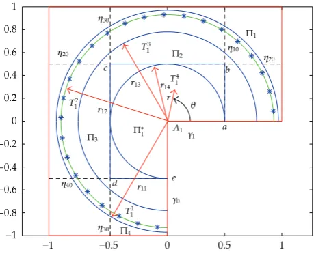
Example 8.1. LetGbe L-shaped and defined as follows:
Gx, y:−1< x <1,−1< y <1\Ω, 8.1
−1 −0.5 0 0.5 1 −1 −0.8 −0.6 −0.4 −0.2 0 0.2 0.4 0.6 0.8 1 A1 T4 1 T1 1 θ T3 1 T2 1 η10
η20 η
20 η30 η30 η40 r14 r13 γ1 r12 γ0 r11 r a b c d e Π2 Π∗ 1 Π1 Π3 Π4
Figure 1:Description of BGM for the L-shaped domain.
We consider the following problem:
Δu0 inG,
uvr, θ onγ, 8.2
where
vr, θ 9
56r
8/3cos
%
8 3θ
&
r2/3sin
%
2 3θ
&
8.3
is the exact solution of this problem.
We choose a “singular” part ofGas
GSx, y:−0.5< x <0.5,−0.5< y <0.5\Ω1, 8.4
whereΩ1 {x, y: 0≤ x≤0.5,−0.5 ≤y≤ 0}.ThenGNS G\GSis a “nonsingular” part
ofG.
The given domainGis covered by four overlapping rectanglesΠk,k1, . . . ,4,and by
the block sectorT3
1 seeFigure 1.For the boundary ofGSonG, that is,t1 the polygonal line
abcdeis taken. The radiusr12 of sectorT12 is taken as 0.93.According to8.3, the function
Qr, θin2.2is
Qr, θ 1
π 9 56 1 0
yt4dt
t−x 2
y2 1 π 9 56 1 0
yt4dt
tx 2
10−5 10−4 10−3 10−2
10−5
10−4
10−3
ε
Maxi
m
u
m
err
or
h=1/16, n=45
a
10−5 10−4 10−3
10−6
10−5
10−4
ε
=1/32, n=75 h
Maxi
m
u
m
err
or
||ζh||(GS) ||ζh||(GNS)
b
Figure 2:Dependence onεforh−116,32.
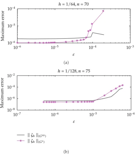
10−6
10−6 10−5 10−4 10−3
10−5
10−4
ε
Maxi
m
u
m
err
or
h=1/64, n=70
a
10−7
10−8
10−6
10−5
10−4
10−2
10−4 ε
Maxi
m
u
m
err
or
h=1/128, n=75
||ζh||(GS)
10−6
||ζh||(GNS)
b
Table 1:The order of convergence in “nonsingular” part whenh2−mandε5×10⁻⁹.
2−m, n ζε
hGNS RmGNS
2−4,70 3.221892×10⁻⁵
3.92
2−5,70 8.21629×10⁻⁶
2−5,45 9.605851×10⁻⁶
4.36
2−6,50 2.198578×10⁻⁶
2−5,70 8.216298×10⁻⁶
3.995
2−6,90 2.056572×10⁻⁶
2−6,45 4.244817×10⁻⁶
4.08
2−7,85 1.037951×10⁻⁶
2−6,75 2.152420×10⁻⁶
3.99
2−7,100 3.387851×10⁻⁷
Table 2:The order of convergence in “singular” part whenh2−mandε5×10⁻⁹.
2−m, n ζε
hGS RmGS
2−4,70 1.5957022×10⁻⁵
4.37
2−5,65 3.6479479×10⁻⁶
2−5,45 8.569069×10⁻⁶
4.11
2−6,50 2.084891×10⁻⁶
2−5,65 3.647947×10⁻⁶
3.97
2−6,100 9.174034×10⁻⁷
2−6,45 4.383277×10⁻⁶
3.96
2−7,85 1.105764×10⁻⁶
2−6,85 2.648988×10⁻⁶
4.18
2−7,100 6.332288×10⁻⁷
Table 3:The minimum errors of the solution over the pairsh−1, nin maximum norm whenε5×10⁻⁹.
h−1, n ζε
hGNS ζhεGS Iteration
16,45 2.567×10⁻⁵ 1.391×10⁻⁵ 15
32,70 8.216×10⁻⁶ 8.732×10⁻⁶ 16
64,70 1.736×10⁻⁶ 1.035×10⁻⁶ 17
128,75 4.038×10⁻⁷ 2.399×10⁻⁷ 17
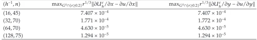
Table 4:The minimum errors of the derivatives over the pairsh−1, nin maximum norm whenε5×10⁻⁹.
h−1, n max
GS∩{r≥0.2}r1/3∂Uε
h/∂x−∂u/∂x maxGS∩{r≥0.2}r1/3∂Uhε/∂y−∂u/∂y
16,45 7.407×10⁻⁴ 7.407×10⁻⁴
32,70 1.771×10⁻⁴ 1.772×10⁻⁴
64,70 4.630×10⁻⁵ 4.630×10⁻⁵
128,75 1.294×10⁻⁵ 1.294×10⁻⁵
wherexr2/3cos2θ/3, andyr2/3sin2θ/3.Since we have only one singular point, we
omitted subindices in8.5. We calculate the valuesQεr
12, θqand Qεr, θon the gridsth1,
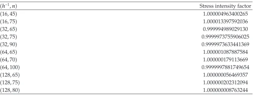
Table 5:The stress intensity factor for the pairsh−1, nwhenε5×10⁻⁹.
h−1, n Stress intensity factor
16,45 1.000004963400265
16,75 1.000013397592036
32,65 0.999994989029130
32,75 0.9999973755906025
32,90 0.9999973633441369
64,65 1.000001087887584
64,70 1.000000179113669
64,100 0.9999997881749654
128,65 1.000000056469357
128,75 1.000000202312094
128,80 1.000000008763244
On the basis of7.5and8.5for the stress intensity factor, we have
τ1ε,n
3 28π
2
n0.932/3
n
q1
uεh0.93, θqj−Qqεj2
sin2 3θ
q
j. 8.6
Taking the zero approximationuεh00,the results of realization of the iteration6.1
for the solution of the problem inExample 8.1are given in Tables1–4. Tables1and2represent the order of convergence
Rm GNS
maxGNSuε
2−m−u
maxGNSuε
2−m1−u
, 8.7
in “nonsingular”, and the order of convergence
Rm GS
maxGSUε2−m−u
maxGSUε
2−m1−u
8.8
in “singular” part ofG,respectively, forε5×10⁻⁹. InTable 3, the minimal values over the
pairsh−1, n,of the errors in maximum norm, of the approximate solution whenε5×10⁻⁹
are presented. The similar values of errors for the first-order derivatives are presented in Table 4 when ∂Q/∂x and ∂Q/∂y are approximated by second-order central difference formula onGS forr ≥ 0.2.For r < 0.2, the order of errors decrease is down to 10−3 which
are not presented inTable 4. This happens because the integrands in8.5are not sufficiently smooth for second-order differentiation formula. The order of accuracy of the derivatives for
r < 0.2 can be increased if we use similar quadrature rules which we used for the integrals in8.5for the derivatives of integrands also.Table 5represents the stress intensity factor for the pairsh−1, nwhenε5×10⁻⁹.
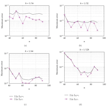
Figures 2 and 3 show dependence on ε for different mesh steps h. Figure 4
40 60 80 100 10−6
10−5
10−4
n
Maxi
m
u
m
err
or
h=1/16
a
40 60 80 100
10−6
10−5
10−4
n
Maxi
m
u
m
err
or
h=1/32
b
40 60 80 100
10−6
10−5
10−4
n
Maxi
m
u
m
err
or
h=1/64
||ζh||(GS)
||ζh||(GNS)
c
40 60 80 100
10−6
10−5
10−7
n
Maxi
m
u
m
err
or
h=1/128
||ζh||(GS)
||ζh||(GNS)
d
Figure 4:Maximum error depending on the number of quadrature nodesn.
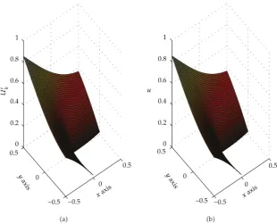
different mesh steps h.The approximate solution and the exact solution in “singular” part are given inFigure 5to illustrate the accuracy of the BGM. The error function forε5×10⁻⁹
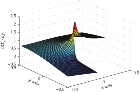
of calculating the functionQr, θin8.5is presented inFigure 6.Figures7and8show the behavior of the first-order partial derivatives of the approximate solution in “singular” part.
9. Conclusions
We have developed the block-grid method for nonanalytic boundary conditions of the first kind on the whole boundary, that is, we remove the restriction on the boundary functions to be algebraic polynomials on the sides of the polygon causing the singular vertices. It is assumed that the boundary function on the whole boundary is given from the H ¨older classesC2,λ,0 < λ < 1.In the integral representations around each singular vertex, which
a b
Figure 5:The approximate solutionUε
hand the exact solutionuin the “singular” part forε5×10− 9.
Figure 6:The error function in “singular” part whenε5×10⁻⁹.
It is proved that the final uniform error is of order Oh2ε, where ε is the error of the
approximation of the mentioned integrals, andhis the mesh step. For thep-order derivatives
p 0,1, . . . of the difference between the approximate and the exact solutions in each
“singular” part, Oh2 εr1/αj−p
j order is obtained. The method is illustrated in solving
Figure 7:∂Uεh/∂xin the “singular” part.
Figure 8:∂Uε
h/∂yin the “singular” part.
the approximate solution and its errors onε, h, and a number of quadrature nodes nare demonstrated.
Acknowledgment
This work was supported by the Ministry of National Education and Culture of TRNC under project MEKB-09-03.
References
1 Z. C. Li,Combined Methods for Elliptic Equations with Singularities, Interfaces and Infinities, vol. 444 of Mathematics and Its Applications, Kluwer Academic Publishers, Dordrecht, The Netherlands, 1998.
2 Z. C. Li and T. T. Lu, “Singularities and treatments of elliptic boundary value problems,”Mathematical and Computer Modelling, vol. 31, no. 8-9, pp. 97–145, 2000.
3 A. A. Dosiyev, “The high accurate block-grid method for solving Laplace’s boundary value problem with singularities,”SIAM Journal on Numerical Analysis, vol. 42, no. 1, pp. 153–178, 2004.
5 A. A. Dosiyev, “A block-grid method of increased accuracy for solving the Dirichlet problem for the Laplace equation in polygons,”Computational Mathematics and Mathematical Physics, vol. 34, no. 5, pp. 591–604, 1994.
6 A. A. Dosiyev and S. Cival, “A difference-analytical method for solving Laplace’s boundary value problem with singularities,” inProceedings of Conference on “Dynamical Systems and Applications”, pp. 339–360, Antalya, Turkey, July 2004.
7 A. A. Dosiyev and S. Cival, “A combined method for solving Laplace’s boundary value problem with singularities,”International Journal of Pure and Applied Mathematics, vol. 21, no. 3, pp. 353–367, 2005.
8 A. A. Dosiyev and S. C. Buranay, “A fourth order accurate difference-analytical method for solving Laplace’s boundary value problem with singularities,” inMathematical Methods in Engineers, K. Tas, J. A. T. Machado, and D. Baleanu, Eds., pp. 167–176, Springer, New York, NY, USA, 2007.
9 E. A. Volkov, “An exponentially converging method of solving the Laplace equation on polygons,” Mathematics of the USSR, Sbornik, vol. 37, no. 3, pp. 295–325, 1980.
10 E. A. Volkov,Block Method for Solving the Laplace Equation and for Constructing Conformal Mappings, CRC Press, Boca Raton, Fla, USA, 1994.
11 G. J. Fix, S. Gulati, and G. I. Wakoff, “On the use of singular functions with finite element approximations,”Journal of Computational Physics, vol. 13, pp. 209–228, 1973.
12 V. A. Kondratiev, “Boundary value problems for elliptic equations in domains with conical or angular points,”Transactions of the Moscow Mathematical Society, vol. 16, pp. 227–313, 1967.
13 P. Grisvard,Elliptic Problems in Nonsmooth Domains, vol. 24 ofMonographs and Studies in Mathematics, Pitman, Boston, Mass, USA, 1985.
14 S. Cho and M. Safonov, “H ¨older regularity of solutions to second-order elliptic equations in nonsmooth domains,”Boundary Value Problems, vol. 2007, Article ID 57928, 24 pages, 2007.
15 E. A. Volkov, “Approximate solution by the block method of the Laplace equation on polygons with nonanalytic boundary conditions,”Proceedings of the Steklov Institute of Mathematics, no. 4, pp. 65–90, 1992.
16 A. A. Dosiyev, “A fourth order accurate composite grids method for solving Laplace’s boundary value problems with singularities,”Computational Mathematics and Mathematical Physics, vol. 42, no. 6, pp. 832–849, 2002.
17 V. P. Mijailov,Partial Differential Equations, Mir, Moscow, Russia, 1978.
18 E. A. Volkov, “The method of composite regular nets for the Laplace equation on polygons,”Trudy Matematicheskogo Instituta imeni V. A. Steklova, vol. 140, pp. 68–102, 1976.
19 E. A. Volkov, “Approximate solution by the block method of the Laplace equation on polygons with analytic mixed boundary conditions,”Proceedings of the Steklov Institute of Mathematics, no. 2, pp. 137– 153, 1994.