Two-Dimension Riemann Initial-Boundary Value Problem of Scalar Conservation Laws with Curved Boundary

Volume 2011, Article ID 138396,16pages doi:10.1155/2011/138396

Research Article

Two-Dimension Riemann Initial-Boundary

Value Problem of Scalar Conservation Laws

with Curved Boundary

Huazhou Chen

_{and Tao Pan}

1_{Department of Mathematics, Shanghai University, Shanghai 200444, China}

2_{Key Laboratory of Optoelectronic Information and Sensing Technologies of Guangdong Higher Educational} Institutes, Jinan University, Guangzhou 510632, China

Correspondence should be addressed to Tao Pan,[email protected]

Received 16 December 2010; Accepted 1 February 2011

Academic Editor: Julio Rossi

Copyrightq2011 H. Chen and T. Pan. This is an open access article distributed under the Creative Commons Attribution License, which permits unrestricted use, distribution, and reproduction in any medium, provided the original work is properly cited.

This paper is concerned with the structure of the weak entropy solutions to two-dimension Riemann initial-boundary value problem with curved boundary. Firstly, according to the definition of weak entropy solution in the sense of Bardos-Leroux-Nedelec 1979, the necessary and sufficient condition of the weak entropy solutions with piecewise smooth is given. The boundary entropy condition and its equivalent formula are proposed. Based on Riemann initial value problem, weak entropy solutions of Riemann initial-boundary value problem are constructed, the behaviors of solutions are clarified, and we focus on verifying that the solutions satisfy the boundary entropy condition. For different Riemann initial-boundary value data, there are a total of five different behaviors of weak entropy solutions. Finally, a worked-out specific example is given.

1. Introduction

Multidimensional conservation laws are a famous hard problem that plays an important role in mechanics and physics 1–3. For Cauchy problem of multi-dimensional scalar conservation laws, Conway and Smoller 4 and Kruzkov 1 have proved that weak solution uniquely exists if it also satisfies entropy condition, and it is called weak entropy solutions. In order to further understand qualitative behavior of solutions, it is also important to investigate multi-dimensional Riemann problems. For two-dimensional case, Lindquist

initial value contains two constant states divided by a curve can not be solved by selfsimilar transformations, and Yang10 proposed a new approach for construction of shock wave and rarefaction wave solutions; especially, rarefaction wave was got by constructing implicit function instead of the usual selfsimilar method. This approach can be expanded to generaln -dimension. In addition, multi-dimensional scalar conservation laws with boundary are more common in practical problems. Bardos et al.2have proved the existence and uniqueness of the weak entropy solution of initial-boundary problems of multi-dimensional scalar conservation laws. The main difficulty for nonlinear conservation laws with boundary is to have a good formation of the boundary condition. Namely, for a fixed initial value, we really can not impose such a condition at the boundary, and the boundary condition is necessarily linked to the entropy condition. Moreover the behavior of solutions for one-dimensional problem with boundary was discussed in11–18. However, for multi-dimensional problem with boundary, the behaviors of solutions are still hard to study.

In this paper, two-dimensional case as an example of Yang’s multi-dimensional Riemann problem10is expanded to the case with boundary. Considering two-dimensional Riemann problem for scalar conservation laws with curved boundary,

ut

∂f1u

∂x1

∂f2u

∂x2

0, x1, x2∈Ω, t >0,

u|_{t 0} u, x1, x2∈Ω,

u|_Γ u−, t >0,

1.1

whereu ut, x1, x2,uandu−are both constants,f1u, f2u∈C2R,Mx1, x2∈C1R2,

Mx1, x2 0 is a smooth manifold and dividesR2 into two infinite parts,Ω {x1, x2 |

Mx1, x2>0}, andΓ {t, x1, x2|Mx1, x2 0, t >0}and denoteu|Γ γu.

InSection 2, weak entropy solution of Riemann initial-boundary value problem1.1

is defined, and the boundary entropy condition is discussed. In Section 3, weak entropy solutions of the corresponding Riemann initial value problem are expressed. In Section 4, using the weak entropy solutions of the corresponding Riemann initial value problem, we construct the weak entropy solutions of Riemann initial-boundary value problem, and prove that they satisfy the boundary entropy condition. The weak entropy solutions include a total of five different shock and rarefaction wave solutions based on different Riemann data. Finally, inSection 5, we give a worked-out specific example.

2. Preliminaries

According to the definition of the weak entropy solution and the boundary entropy condition to the general initial-boundary problems of multi-dimensional scalar conservation laws which was proposed by Bardos et al.2and Pan and Lin13, we can obtain the following definition and three lemmas for Riemann initial-boundary value problem1.1.

Definition 2.1. A locally bounded and bounded variation functionut, x1, x2on0,∞×Ω

the following inequality:

_∞

0

M>0

|u−k|ϕtsgnu−k

f1u−f1k

ϕx1sgnu−k

f2u−f2k

ϕx2

×dx1dx2dt

M>0

|u−k|ϕ0, x1, x2dx1dx2

Γsgnu−−k

f1

γu−f1k, f2

γu−f2k

◦nγϕdx1dx2dt≥0,

2.1

wherenis the outward normal vector of curveMx1, x2.

Lemma 2.2. Ifut, x1, x2is a weak entropy solution of1.1, then it satisfies the following boundary:

entropy condition

sgnγu−u−f1

γu−f1k, f2

γu−f2k

◦n≥0, k∈Iγu, u−, a.e.t >0, 2.2

whereIγu, u− minγu, u−,maxγu, u−.

It can be easily proved that∀k ∈ Iγu, u−,sgnγu−u− sgnγu−k, so2.2can be rewritten as

sgnγu−kf1

γu−f1k, f2

γu−f2k

◦n≥0, k∈Iγu, u−, a.e.t >0, 2.3

thus one can getγu u−or

n◦

f1

γu−f1k

γu−k , f2

γu−f2k

γu−k

≥0, k∈Iγu, u−, k /γu, a.e.t >0, 2.4

and one notices thatn −Mx1,−Mx2,Mx1 ∂Mx1, x2/∂x1, Mx2 ∂Mx1, x2/∂x2, then boundary entropy condition2.2is equivalent to

γu u₋ or

Mx1

f1

γu−f1k

γu−k Mx2

f2

γu−f2k

γu−k ≤0, k∈I

γu, u₋, k /γu, a.e.t >0.

2.5

The proof for one-dimension case ofLemma 2.2can be found in Pan and Lin’s work

13, and the proof forn-dimension case is totally similar to one-dimension case; actually the idea of the proof first appears in Bardos et al.’s work2, so the proof details forLemma 2.2

are omitted here.

Lemma 2.3. A piecewise smooth functionut, x1, x2with smooth discontinuous surface is a weak

(i) Rankine-Hugoniot condition: At any point P on discontinuity surface S of solution ut, x1, x2,NPis a unit normal vector toSatPif

ur lim

ε→0uPεn,

ul lim

ε→0−uPεn,

2.6

then

NP◦

u,f1

,f2

0, 2.7

whereu ur−ul,f1 f1ur−f1ul,f2 f2ur−f2ul.

For any constantk∈ul, ur,P∈S,

NP◦

k−ul, f1k−f1ul, f2k−f2ul

≥0 2.8

or equivalently

NP◦

k−ur, f1k−f1ur, f2k−f2ur

≥0. 2.9

(ii) Boundary entropy condition:

γu u− or

Mx1

f1

γu−f1k

γu−k Mx2

f2

γu−f2k

γu−k ≤0, k∈I

γu, u₋, k /γu, a.e.t >0. 2.10

(iii) Initial value condition:

u0, x1, x2 u0x1, x2, Mx1, x2>0. 2.11

For piecewise smooth solution with smooth discontinuous surface, Rankine-Hugoniot condition2.7, entropy conditions2.8,2.9and initial value condition2.11are obviously satisfied, see also the previous famous works in4,7–9. As inLemma 2.2, boundary entropy condition2.10also holds. The proof of the converse in not difficult and is omitted here.

According to Bardos et al.’s work2, we have the following Lemma.

Lemma 2.4. Ifut, x1, x2 is piecewise smooth weak entropy solution of 1.1 which satisfies the

conditions ofLemma 2.3, thenut, x1, x2is unique.

3. Solution of Riemann Initial Value Problem

First, we study the Riemann initial value problem corresponding to the Riemann initial-boundary value problem1.1as follows:

ut

∂f1u

∂x1

∂f2u

∂x2 0, t >0,

u|_{t 0} ⎧ ⎨ ⎩

u₋, Mx1, x2<0

u, Mx1, x2>0.

3.1

ConditionHForu∈a, b,

Mx1f1 u Mx2f2 u>0, 3.2

wherea, bis a certain intervala, bcan be a finite number or∞.

Condition H combines flux functions f1, f2 and curved boundary manifold M,

providing necessary condition for the convex property of the new flux function which will be constructed in formula 4.5. The convex property clarifies whether the characteristics intersect or not, whether the weak solution satisfied internal entropy conditions2.8and

2.9and boundary entropy condition2.10, In addition, ConditionHis easily satisfied, for example,f1u f2u 1/2u2,Mx1, x2 x31x2, thenMx1f1 uMx2f2 u 3x211>0,

so ConditionHholds. HereMx1, x2 0 is a cubic curve on the X1-X2plane, and it is strictly

bending.

Yang’s work10showed that depending on whether the characteristics intersect or not, the weak entropy solution of3.1has two forms as follows.

Lemma 3.1see10. Suppose (H) holds. Ifu₋ > u, then weak entropy solution of 3.1is shock wave solutionS, and

ut, x1, x2

⎧ ⎪ ⎪ ⎪ ⎪ ⎪ ⎨ ⎪ ⎪ ⎪ ⎪ ⎪ ⎩

u−, M

x1−

f1

ut, x2−

f2

ut

<0,

u, M

x1−

f1

ut, x2−

f2

ut

>0,

3.3

and discontinuity surfaceSt, x1, x2 0is

M

x1−

f1

ut, x2−

f2

ut

0, 3.4

Lemma 3.2see10. Suppose that (H) holds. Ifu− < u, then weak entropy solution of 3.1is

rarefaction wave solutionR, and

ut, x1, x2

⎧ ⎪ ⎪ ⎪ ⎪ ⎪ ⎪ ⎪ ⎨ ⎪ ⎪ ⎪ ⎪ ⎪ ⎪ ⎪ ⎩

u₋, 0> Mx1−f₁u−t, x2−f₂u−t, t >0,

Ct, x1, x2, M

x1−f₁u−t, x2−f2u−t

≥0

≥Mx1−f₁ut, x2−f2ut

, t >0,

u, Mx1−f1ut, x2−f2ut

>0, t >0,

3.5

whereCt, x1, x2is the implicit function which satisfies

Mx1−f1Ct, x2−f2Ct

0. 3.6

Theorem 3.3see10. Suppose that (H) holds. Givenu₋, u ∈a, b, then

iifu₋> u, weak entropy solution of 3.1isSandut, x1, x2has a form as3.3;

iiifu₋< u, weak entropy solution of 3.1isRandut, x1, x2has a form as3.5;

iiiweak entropy solutions formed as3.3and3.5uniquely exist.

The weak entropy solutions constructed here are piecewise smooth and satisfy conditions (i) and (iii) ofLemma 2.3.

4. Solution of Riemann Initial-Boundary Value Problem

Now we restrict the weak entropy solutions of the Riemann initial value problem 3.1

constructed inSection 3in region {t > 0} ×Ω, and they still satisfy conditions iand iii

of Lemma 2.3. If they also satisfy the boundary entropy condition ii ofLemma 2.3, then

they are the weak entropy solutions of Riemann initial-boundary value problem1.1. Based on different Riemann data of u and u₋, the weak entropy solutions of the Riemann initial value problem 3.1 have the following five different behaviors when restricted in region{t >0} ×Ω.

Ifu− > u, the solution of3.1is shock waveSand

ut, x1, x2

⎧ ⎪ ⎪ ⎪ ⎪ ⎪ ⎨ ⎪ ⎪ ⎪ ⎪ ⎪ ⎩

u−, M

x1−

f1

ut, x2−

f2

ut

<0, Mx1, x2>0, t >0,

u, M

x1−

f1

ut, x2−

f2

ut

>0, Mx1, x2>0, t >0.

4.1

Mx1−f1/ut, x2−f2/ut 0 is formed by movingMx1, x2 0 along

the direction of the vector f1/u,f2/u f₁u− f1u−/u −u−,f2u −

f2u−/u−u−α, and the outward normal vectornof curveMx1, x2 0 is equal to

−Mx1,−Mx2. According to the angle betweenαandn, the solution restricted in{t >0} ×Ω

has two behaviors as follows.

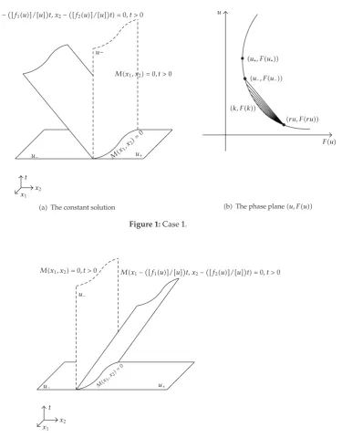
Mx1−f1u/ut, x2−f2u/ut 0, t >0

u−

Mx1, x2 0, t >0

u− Mx u

1, x 2

0

t x2

x1

aThe constant solution

u

Fu u∗, Fu∗

u−, Fu−

k, Fk

ru, Fru

b The phase planeu, Fu Figure 1:Case1.

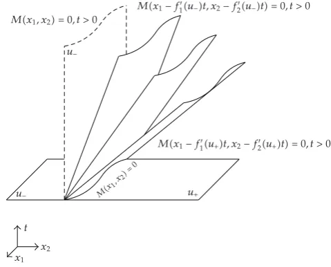
Mx1−

f1u/ut, x2−

f2u/ut 0, t >0

u−

Mx1, x2 0, t >0

u− Mx u

1, x 2

0

t

x2

x1

Figure 2:The shock wave solution of Case2.

See alsoFigure 1a; it shows that the angle between αand n is an acute angle, the shock wave surfaceMx1−f1/ut, x2−f2/ut 0 is outside region{t >0} ×Ω, and

the solution is constant state formed as

ut, x1, x2 u, Mx1, x2≥0, t >0. 4.2

See alsoFigure 2; it shows that the angle betweenαandnis an obtuse angle, the shock wave surfaceMx1−f1/ut, x2−f2/ut 0 is inside region{t >0} ×Ω, and the

solution is shock wave formed as

ut, x1, x2

⎧ ⎪ ⎪ ⎪ ⎪ ⎪ ⎨ ⎪ ⎪ ⎪ ⎪ ⎪ ⎩

u−, Mx1, x2>0> M

x1−

f1

ut, x2−

f2

ut

, t >0

u, M

x1−

f1

ut, x2−

f2

ut

>0, t >0.

4.3

Ifu− < u, the solution of3.1is rarefaction waveRand

ut, x1, x2

⎧ ⎪ ⎪ ⎪ ⎪ ⎪ ⎪ ⎪ ⎪ ⎪ ⎪ ⎪ ⎪ ⎪ ⎪ ⎪ ⎪ ⎪ ⎨ ⎪ ⎪ ⎪ ⎪ ⎪ ⎪ ⎪ ⎪ ⎪ ⎪ ⎪ ⎪ ⎪ ⎪ ⎪ ⎪ ⎪ ⎩

u−, Mx1−f₁u−t, x2−f₂u−t<0,

Mx1, x2>0, t >0,

Ct, x1, x2, M

x1−f₁u−t, x2−f₂u−t≥0,

Mx1−f₁ut, x2−f2ut

≤0, Mx1, x2>0, t >0,

u, Mx1−f1ut, x2−f2ut

>0,

Mx1, x2>0, t >0.

4.4

Mx1−f₁u−t, x2−f₂u−t 0 is formed by movingMx1, x2 0 along the direction

of the vectorf₁u−, f2u− β−,Mx1−f1ut, x2−f2ut 0 is formed by moving

Mx1, x2 0 along the direction of the vectorf₁u, f2uβ, and the outward normal

vectornof curveMx1, x2 0 is equal to−Mx1,−Mx2.

We construct a new flux function

fx1, x2, u Mx1f1u Mx2f2uFu, 4.5

according to conditionH,F u Mx1f1 u Mx2f2 u >0,Fuis convex, andFuis

monotonically increasing function, soFu₋< Fu. And also

Fu− Mx1f1u− Mx2f2u− −n◦

f₁u−, f2u−

,

Fu Mx1f1u Mx2f2u −n◦

f₁u, f₂u. 4.6

Thus,n◦f₁u₋, f₂u₋> n◦f₁u, f₂u. According to the angles betweenβ,β₋, and

n, the solution restricted in{t >0} ×Ωhas three behaviors as follows.

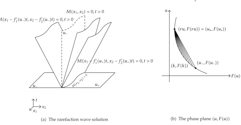
Mx1−f1u−t, x2−f2u−t 0, t >0

u−

Mx1, x2 0, t >0

u− Mx u

1, x2

0

Mx1−f1ut, x2−f2ut 0, t >0

t

x2

x1

Figure 3:The rarefaction wave solution of Case3.

See alsoFigure 3; it shows that the angles betweenβ,β−,andnare obtuse angles, the

rarefaction wave surfacesMx1−f₁ut, x2−f₂ut 0 andMx1−f₁u−t, x2−f₂u−t 0

are both inside region{t >0} ×Ω, and the solution is rarefaction wave formed as

ut, x1, x2

⎧ ⎪ ⎪ ⎪ ⎪ ⎪ ⎪ ⎪ ⎨ ⎪ ⎪ ⎪ ⎪ ⎪ ⎪ ⎪ ⎩

u−, Mx1, x2>0> M

x1−f1u−t, x2−f2u−t

, t >0,

Ct, x1, x2, M

x1−f₁u−t, x2−f₂u−t≥0

≥Mx1−f₁ut, x2−f₂ut, t >0,

u, Mx1−f₁ut, x2−f₂ut>0, t >0,

4.7

whereCt, x1, x2is the implicit function which satisfies3.6.

Case 4. Ifu₋ < uandn◦f₁u, f₂u<0< n◦f₁u₋, f₂u₋.

See alsoFigure 4a; it shows that the angle betweenβandnis an obtuse angle, the

angle betweenβ₋andnis an acute angles, the rarefaction wave surfaceMx1−f₁ut, x2−

f₂ut 0 is inside region{t > 0} ×Ω, the rarefaction wave surfaceMx1−f₁u−t, x2−

f₂u−t 0 is outside region{t >0} ×Ω, and the solution is rarefaction wave formed as

ut, x1, x2

⎧ ⎨ ⎩

Ct, x1, x2, Mx1, x2>0≥M

x1−f1ut, x2−f2ut

, t >0,

u, Mx1−f1ut, x2−f2ut

>0, t >0,

4.8

whereCt, x1, x2is the implicit function which satisfies3.6.

Mx1−f1u−t, x2−f2u−t 0, t >0

u−

Mx1, x2 0, t >0

u− Mx u

1, x2

0

Mx1−f1ut, x2−f2ut 0, t >0

t x2

x1

a The rarefaction wave solution

u

Fu ru, Fru u∗, Fu∗

u−, Fu− k, Fk

b The phase planeu, Fu Figure 4:Case4.

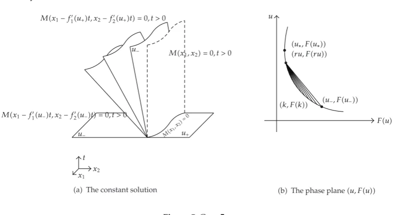
See alsoFigure 5a; it shows that the angles betweenβ,β₋, andnare acute angles, the rarefaction wave surfacesMx1−f1ut, x2−f2ut 0 andMx1−f1u−t, x2−f2u−t 0

are both outside region{t >0} ×Ω, and the solution is constant state formed as

ut, x1, x2 u, Mx1, x2>0, t >0. 4.9

Next, we verify the above five solutions all satisfying the boundary entropy condition

ii of Lemma 2.3. By noticing the definition of Fu 4.5 and its convex property, the

boundary entropy conditioniiofLemma 2.3can be equivalent to the following formula

γu u− or F

γu − Fk

γu−k ≤ 0, k∈I

γu, u−, k /γu, a.e.t >0, 4.10

and thus we verify the above five solutions all satisfying the boundary entropy condition

4.10.

Case 1. Whenu−> u,n◦f1/u,f2/u≥0, the shock wave solution is formed as4.2.

In this case,γu u/u−since

Fγu−Fu−

γu−u− −n◦

f1

u,

f2

u

≤0see also Figure 1b, 4.11

andγu < u₋ ≤u_∗, whereu_∗is the extreme point ofFu. For∀k∈γu, u₋, according to the convex property ofFu, we have that

Fγu−Fk γu−k ≤

Fγu−Fu₋

γu−u− ≤0, 4.12

Mx1−f1u−t, x2−f2u−t 0, t >0

u− _Mx

1, x2 0, t >0

u− Mx u

1, x 2

0

Mx1−f1ut, x2−f2ut 0, t >0

t x2

x1

a The constant solution

u

Fu u∗, Fu∗

ru, Fru

u−, Fu− k, Fk

bThe phase planeu, Fu

Figure 5:Case5.

Case 2. Whenu−> u,n◦f1/u,f2/u<0, the shock wave solution is formed as4.3.

In this case,γu u₋, so the boundary entropy condition4.10is naturally verified.

Case 3. When u− < u,n◦f1u, f2u < n◦f1u−, f2u− ≤ 0, the rarefaction wave

solution is formed as4.7. In this case,γu u−, and so the boundary entropy condition

4.10is naturally verified.

Case 4. When u− < u,n ◦f1u, f2u < 0 < n◦f1u−, f2u−, the rarefaction wave

solution is formed as4.8. In this case,γu Ct, x1, x2|Mx1,x2 0 u∗ ≤ u−,Fu∗ 0 and

Fu− −n◦f1u−, f2u− < 0 < −n◦f1u, f2u Fu see also Figure 4b,

namely,Fu−< Fγu 0 < Fu. For∀k ∈u−, γu, according to the convex property of

Fuand Lagrange mean value theorem, there existsξ∈k, γu, satisfying

Fγu−Fk

γu−k Fξ≤F

γu 0, 4.13

and so the boundary entropy condition4.10is verified.

Case 5. When u− < u, 0 ≤ n ◦f1u, f2u < n◦f1u−, f2u−, the rarefaction wave

solution is formed as4.9. In this case,γu u > u₋ sinceFu₋ −n◦f₁u₋, f₂u₋ < −n◦f₁u, f2u Fγu ≤ 0see alsoFigure 5bFor∀k ∈u−, γu, according to the

convex property ofFuand Lagrange mean value theorem, there existsξ∈k, γu, satisfying

Fγu−Fk

γu−k Fξ≤F

γu≤0, 4.14

In summary, we have the following theorem.

Theorem 4.1. Suppose that (H) holds. Givenu₋, u ∈a, b, then

iifu₋> uandn◦f1/u,f2/u≥0, the solution of 1.1is constant state and has

form as4.2,

iiifu−> uandn◦f1/u,f2/u<0, the solution of1.1is shock waveS, and has

form as4.3,

iiiifu− < uandn◦f1u, f2u< n◦f1u−, f2u−≤ 0, the solution of 1.1is

rarefaction waveRand has a form as4.7,

ivifu− < uandn◦f1u, f2u< 0< n◦f1u−, f2u−, the solution of 1.1is

rarefaction waveRand has a form as4.8;

vifu₋ < uand0≤ n◦f₁u, f₂u< n◦f₁u₋, f₂u₋, the solution of 1.1is constant state and has a form as4.9.

In addition the solutions formed as4.2,4.3,4.7,4.8, and4.9uniquely exist.

Corollary 4.2. Suppose thatMx1f1 u Mx2f2 u<0foru∈a, b.a, bcan be finite or∞, and

whenu−, u∈a, b,

iifu− > uandn◦f1u, f2u< n◦f1u−, f2u−≤ 0, the solution of 1.1is

rarefaction waveRand has a form as4.7,

iiifu− > uand n ◦f1u, f2u < 0 < n◦f1u−, f2u−, the solution of 1.1is

rarefaction waveRand has a form as4.8,

iiiifu₋ > uand0≤ n◦f₁u, f₂u< n◦f₁u₋, f₂u₋, the solution of 1.1is constant state and has a form as4.9,

ivifu−< uandn◦f1/u,f2/u≥0, the solution of 1.1is constant state and has

a form as4.2,

vifu−< uandn◦f1/u,f2/u<0, the solution of1.1is shock waveSand has

a form as4.3.

Corollary 4.3. The approach here for two-dimensional Riemann initial-boundary problem can be expanded to the case of generaln-dimension.

5. An Example

Solve the following Riemann initial-boundary problem:

ut

u2

2

x1

u2

2

x2

0, x1, x2∈Ω, t >0,

u|_{t 0} u, x1, x2∈Ω,

u|_Γ u−, t >0,

where Mx1, x2 x₁3x2,Ω {x1, x2 | Mx1, x2 > 0}, Γ {t, x1, x2 | Mx1, x2

0, t > 0}, and it denotesu|_Γ γu. Sincef1u f2u 1/2u2, we easily getMx1f1 u

Mx2f2 u 3x211>0, and conditionHholds.

According to the different data ofu andu−, the behavior of the solution to Riemann

initial-boundary problem 5.1 has a total of five situations; they can be described by the following five cases:iu₋ 1,u −2;iiu₋ 2,u −1;iiiu₋ 1,u 2;ivu₋ −1,

u 1;vu− −2,u −1.

For casei,u−> uand

n◦ f1 u, f2 u

−Mx1

f1

u −Mx2

f2

u

−3x2₁f1u−−f1u u−−u −

f2u−−f2u

u−−u

−1

2

3x2₁1u−u

1 2

3x2₁1>0,

5.2

and thus the solution is constant state formed as

ut, x1, x2 −2, x13x2>0, t >0. 5.3

For caseii,u₋> uand

n◦ f1 u, f2 u

−Mx1

f1

u −Mx2

f2

u

−3x2₁f1u−−f1u u−−u −

f2u−−f2u

u−−u

−1

2

3x2₁1u₋u

−1

2

3x2₁1<0,

5.4

and thus the solution is shock wave solution formed as

ut, x1, x2

⎧ ⎪ ⎪ ⎪ ⎪ ⎨ ⎪ ⎪ ⎪ ⎪ ⎩

2, x3

1x2>0>

x1−

1 2t

3

x2−

1 2t

, t >0,

−1,

x1−

1 2t

3

x2−

1 2t

>0, t >0.

For caseiii,u−< uand

n◦f₁u₋, f₂u₋ −Mx1f1u−−Mx2f2u− −

3x2 11

,

n◦f₁u, f2u

−Mx1f1u−Mx2f2u −2

3x2₁1,

5.6

namely,n◦f₁u, f₂u < n◦f₁u₋, f₂u₋ ≤ 0, thus the solution is rarefaction wave formed as

ut, x1, x2

⎧ ⎪ ⎪ ⎪ ⎨ ⎪ ⎪ ⎪ ⎩

1, x3₁x2 >0>x1−t3 x2−t, t >0

Ct, x1, x2, x1−t3 x2−t≥0≥x1−2t3 x2−2t, t >0

2, x1−2t3 x2−2t>0, t >0.

5.7

Here, we only need to solveCt, x1, x2∈ΩC, where

ΩC

t, x1, x2|x1−t3 x2−t≥0≥x1−2t3 x2−2t, t >0

. 5.8

To solve the following equation ofC:

Mx1−f1Ct, x2−f2Ct

x1−Ct3 x2−Ct 0, 5.9

using Cardano formula, we can get the unique solution as

Ct, x1, x2 √₃1

2t ⎡ ⎢ ⎣3

_−x

1−x2

4

27 x1−x2

2

3 _−x

1−x2−

4

27 x1−x2

2

⎤ ⎥ ⎦x1

t .

5.10

SinceCt, x1, x2is the solution of implicit function, we still need to verifyCt, x1, x2

satisfying the following three conditions:aCtCCx1CCx2 0,t, x1, x2 ∈ΩC;bC

1 u−,x1−t3 x2−t 0, t >0;cC 2 u,x1−2t3 x2−2t 0, t >0. In fact,

according to the next proposition, the above three conditions can be easily verified, and the detail the omitted here.

Proposition 5.1. For any real number x, the following formula holds:

3

−xx3

4

27 xx3

2 3

−xx3−

4

27 xx3

2√3

Proof. Let

p 3

−xx3

4

27 xx

32 3

−xx3₋

4

27 xx

32_, 5.12

thenpsatisfies

Epp3√34p2xx3 0, 5.13

wherepmust be one root of5.13. In fact,Ep 3p2√3

4>0. Equation5.13at most has one real root; but−√3

2xis its real root, thusp −√3

2x, and the proposition holds.

For caseiv,u− < uand

n◦f₁u−, f2u−

−Mx1f1u−−Mx2f2u− 3x121,

n◦f₁u, f2u

−Mx1f1u−Mx2f2u −

3x2₁1,

5.14

namely,n◦f₁u, f2u<0< n◦f1u−, f2u−, and thus the solution is rarefaction wave

formed as

ut, x1, x2

⎧ ⎨ ⎩

Ct, x1, x2, x3₁x2>0≥x1−t3 x2−t, t >0

1, x1−t3 x2−t>0, t >0,

5.15

whereCt, x1, x2has the same form as5.10.

For casev,u₋< uand

n◦f₁u−, f2u−

−Mx1f1u−−Mx2f2u− 2

3x2₁1,

n◦f₁u, f2u

−Mx1f1u−Mx2f2u 3x121,

5.16

namely, 0≤n◦f₁u, f₂u< n◦f₁u₋, f₂u₋, and thus the solution is constant state formed as

ut, x1, x2 −1, x13x2>0, t >0. 5.17

Acknowledgment

References

1 S. N. Kruzkov, “Generalized solutions of the Cauchy problem in the large for nonlinear equations of first order,”Soviet Mathematics Doklady, vol. 10, pp. 785–788, 1969.

2 C. Bardos, A. Y. le Roux, and J.-C. N´ed´elec, “First order quasilinear equations with boundary conditions,”Communications in Partial Differential Equations, vol. 4, no. 9, pp. 1017–1034, 1979. 3 P. A. Razafimandimby and M. Sango, “Weak solutions of a stochastic model for two-dimensional

second grade fluids,”Boundary Value Problems, vol. 2010, Article ID 636140, 47 pages, 2010.

4 E. Conway and J. Smoller, “Clobal solutions of the Cauchy problem for quasi-linear first-order equations in several space variables,”Communications on Pure and Applied Mathematics, vol. 19, pp. 95–105, 1966.

5 W. B. Lindquist, “The scalar Riemann problem in two spatial dimensions: piecewise smoothness of solutions and its breakdown,”SIAM Journal on Mathematical Analysis, vol. 17, no. 5, pp. 1178–1197, 1986.

6 D. H. Wagner, “The Riemann problem in two space dimensions for a single conservation law,”SIAM Journal on Mathematical Analysis, vol. 14, no. 3, pp. 534–559, 1983.

7 T. Zhang and Y. X. Zheng, “Two-dimensional Riemann problem for a single conservation law,”

Transactions of the American Mathematical Society, vol. 312, no. 2, pp. 589–619, 1989.

8 J. Guckenheimer, “Shocks and rarefactions in two space dimensions,”Archive for Rational Mechanics and Analysis, vol. 59, no. 3, pp. 281–291, 1975.

9 Y. Zheng, Systems of Conservation Laws: Two-Dimensional Riemann Problems, vol. 38 of Progress in Nonlinear Differential Equations and Their Applications, Birkh¨auser, Boston, Mass, USA, 2001.

10 X. Yang, “Multi-dimensional Riemann problem of scalar conservation law,”Acta Mathematica Scientia, vol. 19, no. 2, pp. 190–200, 1999.

11 F. Dubois and P. LeFloch, “Boundary conditions for nonlinear hyperbolic systems of conservation laws,”Journal of Differential Equations, vol. 71, no. 1, pp. 93–122, 1988.

12 P. LeFloch and J.-C. N´ed´elec, “Explicit formula for weighted scalar nonlinear hyperbolic conservation laws,”Transactions of the American Mathematical Society, vol. 308, no. 2, pp. 667–683, 1988.

13 T. Pan and L. Lin, “The global solution of the scalar nonconvex conservation law with boundary condition,”Journal of Partial Differential Equations, vol. 8, no. 4, pp. 371–383, 1995.

14 T. Pan and L. Lin, “The global solution of the scalar nonconvex conservation law with boundary condition.Continuation,”Journal of Partial Differential Equations, vol. 11, no. 1, pp. 1–8, 1998. 15 T. Pan, H. Liu, and K. Nishihara, “Asymptotic stability of the rarefaction wave of a one-dimensional

model system for compressible viscous gas with boundary,”Japan Journal of Industrial and Applied Mathematics, vol. 16, no. 3, pp. 431–441, 1999.

16 T. Pan and Q. Jiu, “Asymptotic behaviors of the solutions to scalar viscous conservation laws on bounded interval corresponding to rarefaction waves,”Progress in Natural Science, vol. 9, no. 12, pp. 948–952, 1999.

17 T. Pan and H. Liu, “Asymptotic behaviors of the solution to an initial-boundary value problem for scalar viscous conservation laws,”Applied Mathematics Letters, vol. 15, no. 6, pp. 727–734, 2002. 18 T. Pan, H. Liu, and K. Nishihara, “Asymptotic behavior of a one-dimensional compressible viscous