www.astra-proceedings.net/2/51/2015/ doi:10.5194/ap-2-51-2015
© Author(s) 2015. CC Attribution 3.0 License.
A solution to the cosmic ray anisotropy problem
P. Mertsch1and S. Funk2
1Kavli Institute for Particle Astrophysics & Cosmology, 2575 Sand Hill Road, M/S 29,
Menlo Park, CA 94025, USA
2Erlangen Center for Astroparticle Physics (ECAP), Friedrich-Alexander Universität Erlangen-Nürnberg,
Erlangen, Germany
Correspondence to: P. Mertsch ([email protected])
Received: 28 May 2015 – Revised: 12 August 2015 – Accepted: 9 September 2015 – Published: 8 October 2015
Abstract. Observations of the cosmic ray (CR) anisotropy are widely advertised as a means of finding nearby sources. This idea has recently gained currency after the discovery of a rise in the positron fraction and is the goal of current experimental efforts, e.g., with AMS-02 on the International Space Station. Yet, even the anisotropy observed for hadronic CRs is not understood, in the sense that isotropic diffusion models overpredict the dipole anisotropy in the TeV–PeV range by almost two orders of magnitude. Here, we consider two additional effects normally not considered in isotropic diffusion models: anisotropic diffusion due to the presence of a background magnetic field and intermittency effects of the turbulent magnetic fields. We numerically explore these effect by tracking test-particles through individual realisations of the turbulent field. We conclude that a large misalignment between the CR gradient and the background field can explain the observed low level of anisotropy.
1 Introduction
Information on sources and transport of cosmic rays (CRs) are gained from three types of observations: spectra, com-position and anisotropies. Among those three, anisotropies have a somewhat paradoxical status: on the one hand the observed arrival directions of CRs posses a low level of anisotropy – about 1 part in 1000 or 10 000 at TeV–PeV ener-gies. Given the likely inhomogeneous distribution of sources in the Galaxy, this requires an efficient mechanism to ran-domise the directions of CRs and therefore constrains mod-els of CR transport. On the other hand, a residual anisotropy in the arrival direction encodes information about the posi-tion and age of sources. This has been considered as a pos-sibility for finding nearby sources, in particular in the con-text of the observed rise in the positron fraction. We note that this situation is somewhat reminiscent of the cosmic mi-crowave background (CMB): while the angular power spec-trum of anisotropies contains information on the parameters of the cosmological model, the high level of isotropy requires a mechanism that allows far away regions to be in causal con-tact at early times.
It has been known for a long time that pitch-angle scatter-ing mediated by resonant interaction between CRs and tur-bulent magnetic fields can provide the necessary randomisa-tion (as reviewed by, e.g., Ginzburg et al., 1990). Pitch-angle scattering is also mediating spatial diffusion and if the distri-bution of sources is asymmetric with respect to the observer, e.g. there are more sources towards the Galactic centre than towards the anti-centre, a small degree of residual anisotropy is expected. The amplitudea of the dipole in the arrival di-rections, defined as the relative difference of observed max-imum and minmax-imum fluxes,φmaxandφmin, is related to the
gradient in the isotropic partf0of the distribution function f(x,p,µ)=f0(x,p) (1+a µ),
a=φmax−φmin
φmax+φmin
'3D
v
|∇f0| f0
, (1)
whereDis the isotropic diffusion coefficient andvthe parti-cle speed.
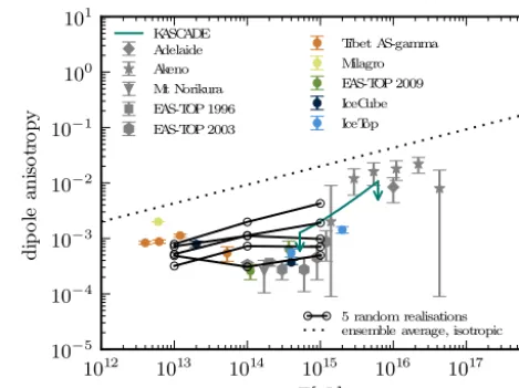
This picture, however, does not compare well with measure-ments (Antoni et al., 2003; Gerhardy et al., 1984; Kifune et al., 1985; Nagashima et al., 1990; Aglietta et al., 1996, 2003; Amenomori et al., 2005; Abdo et al., 2009; Aglietta, 2009; Abbasi, 2012; Aartsen et al., 2013). As shown in Fig. 1, a prediction from the isotropic diffusion model (dotted line, cf. Blasi and Amato, 2012) is almost two orders of mag-nitude higher than the measurements between 100 TeV and 1 PeV. This discrepancy has come to be known as the cosmic ray anisotropy problem (Hillas, 2005; Ptuskin et al., 2006; Pohl et al., 2012; Evoli et al., 2012). Nevertheless, using the observed distribution of arrival directions, in particular the dipole has been widely advertised as a means to infer the presence of young, nearby sources (Buesching et al., 2008; Sveshnikova, 2013; DiBernardo et al., 2011; Borriello et al., 2010; Linden and Profumo, 2013).
In the following we suggest two modifications to the theo-retical picture that in combination can decrease the predicted anisotropy and bring it into agreement with observations. First, in the presence of a background magnetic fieldB0and
for low levels of turbulence – defined as the ratio of turbulent energy density and total energy density,η=δB2/(B02+δB2) – diffusion is inherently anisotropic, with the diffusion along
B0 much more efficient than perpendicular to it. Instead of
Eq. (1), the dipole amplitude should read (see, e.g. Ginzburg et al., 1990)
a=
3 2
1 R
−1
dµµf(µ)
f0
=3
v
|∂f0/∂x| f0
Dk. (2)
Note that now the amplitude depends on the parallel diffu-sion coefficientDkand the CR gradient alongB0(assumed
to be in the x direction). This introduces a new degree of freedom, the angle between B0and the CR gradient
direc-tion∇f0/|∇f0|.
Second, the intermittency in the turbulent magnetic field can play a role. Analytical computations of the transport of CRs can only predict the average distribution functionf for an ensemble of turbulent magnetic fields. Due to the stochas-tic nature of the turbulent fields, in one parstochas-ticular realisation of the turbulent magnetic field we expect deviations from the ensemble average and consequently also deviations of the dipole direction and amplitude from the ensemble averaged direction and amplitude. We note that such intermittency ef-fects have also been argued to be the cause of the CR small scale anisotropy observed at TeV–PeV energies (Giacinti and Sigl, 2011; Ahlers, 2013; Ahlers and Mertsch, 2015).
2 Methodology
We explore both these effects, i.e., the anisotropic diffu-sion and turbulence intermittency effects, by numerically back-tracking particles through individual realisations of a turbulent magnetic field. Given a large number of
trajec-1012 1013 1014 1015 1016 1017 1018 E[eV]
10−5 10−4 10−3 10−2 10−1 100 101
dip
ole
anisotrop
y
KASCADE Adelaide Akeno Mt Norikura EAS-TOP 1996 EAS-TOP 2003
Tibet AS-gamma Milagro EAS-TOP 2009 IceCube IceTop
5 random realisations ensemble average, isotropic
Figure 1.Comparison between measurements of the dipole ampli-tude (Antoni et al., 2003; Gerhardy et al., 1984; Kifune et al., 1985; Nagashima et al., 1990; Aglietta et al., 1996, 2003; Amenomori et al., 2005; Abdo et al., 2009; Aglietta, 2009; Abbasi, 2012; Aart-sen et al., 2013) and models: the dotted line shows the prediction from an isotropic diffusion model (Blasi and Amato, 2012), the open black circles show the dipole anisotropy in five random re-alisations of the turbulent magnetic field for an angle between CR gradient and background magnetic field close to 90◦.
tories, {xi(t), pi(t)}, we can compute the arrival
direc-tions seen by an observer at positionxobs and timet0from
an assumed quasi-stationary CR distribution at an earlier time (t0−1t) and exploiting Liouville’s theorem:f(xobs, pi(t0))=f(xi(t0−1t),pi(t0−1t)). Note the intermittency
effect is due to the local configuration of the turbulent mag-netic field, i.e., the arrival directions can only reflect the turbulent field over the last few scattering lengths. This justifies truncating the expansion of the spatial distribu-tion after the first derivative, i.e., the CR gradient ∇f0.
Therefore, we adopt the quasi-stationary distribution f(x,
t0−1t)=f0+x ∂f0/∂x. Note that in general there is an
an-gle between the gradient direction∇f0/|∇f0|andB0.
We solve the relativistic equations of motions with a 5th order adaptive Runge–Kutta algorithm (Sutherland et al., 2010) at three energies, 10, 100 and 1000 TV. For the level of turbulence we considerη=1 and 0.1 which should bracket its uncertainty. To bridge the large dynamical range between the particle gyroradius and a few times its scattering length, we set up the turbulent magnetic field on a set of nested grids (Giacinti et al., 2011), assuming a Kolmogorov spectrum, an outer scaleL=100 pc and a total RMS field strength of 4 µG.
3 Results
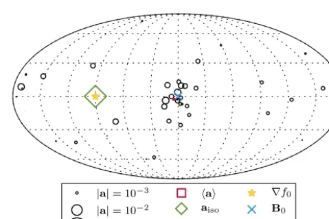
In Fig. 2 we show the dipole directions in 50 realisations of the turbulent magnetic field in the absence ofB0for 1 PeV
re-|a|= 10−3 |a|= 10−2 |a|= 10−1
hai aiso ∇f0
Figure 2. Dipole directions (centres of circles) and amplitudes (radii of circles) in 50 random realisations of the local turbulent magnetic field at 1 PV and forη=1. The CR gradient is denoted by the yellow star, the prediction from an isotropic diffusion model by the green diamond and the average of the 50 random realisations by the red square.
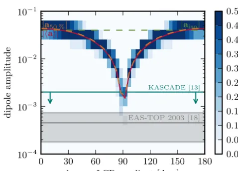
spectively. Two things are noteworthy: It is clear that the indi-vidual dipole directions are in general not pointing in the CR gradient direction (denoted by the yellow star). Second, there is some scatter also in the amplitude of individual dipoles. The (vectorial) mean, however, shown by the red square, is in good agreement both with the expected direction and am-plitude. For all energies considered, the ensemble averaged dipole amplitude reproduces the result of Blasi and Amato (2012), cf. dotted line in Fig. 1. We further explore the scatter in the amplitude in Fig. 3 that shows the distribution of dipole amplitudes as a function of the longitude of the CR gradient direction. (As there is no other direction in this setup, we would not expect any systematic dependence on this direc-tion which is in fact the case.) The dipole amplitudes scatter by a factor of a few around the expectation value |hai|that is always in agreement with the prediction from the isotropic diffusion model, |aiso|. Still, the predictions are at least an
order of magnitude above the upper limit from KASCADE. Figure 4 shows the distribution of dipole directions and amplitudes in the presence ofB0withη=0.1, i.e., a weak
turbulent field, and assuming an angle of∼90◦between∇f0
andB0. The amplitudes are significantly suppressed and the
directions show again a large scatter, but now cluster around the B0direction, indicated by the blue cross, which is also
the direction of the ensemble average dipole. From Fig. 5, it can be seen how the distribution of dipole amplitudes de-pends on the angle betweenB0and∇f0: for small angles,
the amplitudes closely track the prediction from the isotropic diffusion model, with relatively little scatter. At angles close to 90◦though, the amplitude can be significantly suppressed, at the minimum limited only by the level of turbulence η. For the adoptedη=0.1, the mean amplitude is in agreement with KASCADE. We also note that the scatter is enhanced
0 30 60 90 120 150 180
long. of CR gradient [deg.] 10−4
10−3
10−2 10−1
dip
ole
amplitude KASCADE [13]
EAS-TOP 2003 [18]
|aiso| |hai|
|a50 %|
0.00 0.05 0.10 0.15 0.20 0.25 0.30 0.35 0.40 0.45 0.50
Figure 3.Distribution of dipole amplitudes at 1 PV and forη=1 as a function of the longitude of the CR gradient. Each vertical slice is normalised to one. The orange dashed, red solid and green dashed lines show the median, the amplitude of the vectorial mean and the prediction for isotropic diffusion, respectively. The KASCADE up-per limit and EAS-TOP measurement at∼1 PeV are denoted by the cyan solid line and grey band, respectively.
|a|= 10−3 |a|= 10−2 |a|= 10−1
hai aiso
∇f0 B0
Figure 4.Same as Fig. 2, but with a non-zero regular field (η=0.1), indicated by the blue cross.
for angles around 90◦. About 20 % of the turbulent field re-alisations lead to a dipole amplitude that is compatible with the EAS-TOP measurement.
0 30 60 90 120 150 180 long. of CR gradient [deg.] 10−4
10−3 10−2
10−1
dip
ole
amplitude KASCADE [13]
EAS-TOP 2003 [18]
|aiso| |hai|
|a50 %|
0.00 0.05 0.10 0.15 0.20 0.25 0.30 0.35 0.40 0.45 0.50
Figure 5.Same as Fig. 3, but with a non-zero regular field (η=0.1). The ensemble average|hai|follows the prediction from anisotropic diffusion,|hai| ∝p(ν/0)2+cos2ψ whereν,0andψ are the scattering rate, gyrofrequency and angle betweenB0and∇f0(i.e., the longitude of the CR gradient in our setup), respectively.
4 Conclusions
Observations of the dipole direction in the arrival distribution of CRs have been promoted as a means of source searches, yet the measured dipole amplitude is systematically over-predicted by isotropic diffusion models. We suggest two ef-fects, that can resolve this so-called anisotropy problem: the anisotropic nature of diffusion in the presence of a back-ground magnetic field and intermittency, that is fluctuations of the distribution function across individual realisations of the turbulent field. While the conjunction of both effects can sufficiently suppress the dipole amplitude (for small turbu-lence level η and if the background field and CR gradient are close to perpendicular), this is also casting doubt on the chances of finding sources in the dipole direction: in the high turbulence level case (η=1) the directions scatter signifi-cantly around the CR gradient direction (see Fig. 2). In the low turbulence case (η=0.1), there is also scatter and in gen-eral the dipole directions cluster around the field direction, not the gradient direction. For the preferred case with a large angle between gradient and field, see Fig. 3, the scatter is so large that not even the field direction can be inferred.
Acknowledgements. We would like to thank Markus Ahlers
for stimulating discussions. P. Mertsch is supported by DoE contract DE-AC02-76SF00515 and a KIPAC Kavli Fellowship. We acknowledge use of theHEALPixpackage (Gorski et al., 2005).
Edited by: P. Desiati
Reviewed by: M. Ahlers and L. Drury
References
Aartsen, M. G., Abbasi, R., Abdou, Y., et al. (IceCube Collabora-tion): Observation of Cosmic Ray Anisotropy with the IceTop Air Shower Array, Astrophys. J., 765, 55, 2013.
Abbasi, R., Abdou, Y., Abu-Zayyad, T., et al. (IceCube Collabora-tion): Observation of an Anisotropy in the Galactic Cosmic Ray arrival direction at 400 TeV with IceCube, Astrophys. J., 746, 33, 2012.
Abdo, A. A., Allen, B. T., Aune, T., Berley, D., Casanova, S., Chen, C., Dingus, B. L., and Ellsworth, R. W.: The Large Scale Cosmic-Ray Anisotropy as Observed with Milagro, Astrophys. J., 698, 2121–2130, 2009,
Aglietta, M., Alessandro, B., Antonioli, P., Arneodo, F., Bergam-asco, L., Bertaina, M., Bosio, A., Castellina, A., Castagnoli, C., Chiavassa, A., Cini Castagnoli, G., D’Ettorre Piazzoli, B., di Sci-ascio, G., Fulgione, W., Galeotti, P., Ghia, P. L., Iacovacci, M., Mannocchi, G., Melagrana, C., Mengotti Silva, N., Morello, C., Navarra, G., Riccati, L., Saavedra, O., Trinchero, G. C., Vallania, P., Vernetto, S., and EAS-Top Collaboration: A Measurement of the solar and sidereal cosmic ray anisotropy atE(0) approxi-mates 10**14-eV, Astrophys. J., 470, 501–505, 1996.
Aglietta, M., Alekseenko, V. V., Alessandro, B., Antonioli, P., Ar-neodo, F., Bergamasco, L., Bertaina, M., Bonino, R., Castellina, A., Chiavassa, A., D’Ettorre Piazzoli, B., Di Sciascio, G., Ful-gione, W., Galeotti, P., Ghia, P. L., Iacovacci, M., Mannocchi, G., Morello, C., Navarra, G., Saavedra, O., Stamerra, A., Trinchero, G. C., Valchierotti, S., Vallania, P., Vernetto, S., and Vigorito, C.: Evolution of the cosmic ray anisotropy above 1014eV, Astro-phys. J., 692, L130–L133, 2009.
Aglietta, M., Alessandron, B., Antonioli, P., Arneodo, F., Bergam-asco, L., Bertaina, M., Castagnoli, C., Castellina, A., Chiavassa, A., Castagnoli, G. C., D’Ettore Piazzoli, B., Di Sciascio, G., Ful-gione, W., Galeotti, P., Ghia, P. L., Iacovacci, M., Mannocchi, G., Morello, C., Navarra, G., Saavedra, O., Trinchero, G. C., Valchierotti, S., Vallania, P., Vernetto, S., Vigorito, C., and EAS-TOP Collaboration: The cosmic ray anisotropy between 10**14-eV and 10**15-10**14-eV, Proc. 28th Int. Cosmic Ray Conf., Tsukuba, 183–186, 2003.
Ahlers, M.: Anomalous Anisotropies of Cosmic Rays from Turbulent Magnetic Fields, Phys. Rev. Lett., 112, 021101, doi:10.1103/PhysRevLett.112.021101, 2014.
Ahlers, M. and Mertsch, P.: Small-Scale Anisotropies of Cosmic Rays from Relative Diffusion, arXiv:1506.05488 [astro-ph.HE], 2015.
Y., Zhang, Y.; Zhaxisangzhu, Zhou, X. X., and Tibet Asy Collab-oration: Large-scale sidereal anisotropy of Galactic cosmic-ray intensity observed by the Tibet air shower array, Astrophys. J., 626, L29–L32, 2005.
Antoni, T., Apel, W. D., Badea, A. F., Bekk, K., Bercuci, A., Blümer, H., Bozdog, H., Brancus, I. M., Büttner, C., Daumiller, K., Doll, P., Engel, R., Engler, J., Fessler, F., Gils, H. J., Glasstet-ter, R., Haungs, A., Heck, D., Hörandel, J. R., Kampert, K.-H., Klages, H. O., Maier, G., Mathes, H. J., Mayer, H. J., Milke, J., Müller, M., Obenland, R., Oehlschläger, J., Ostapchenko, S., Petcu, M., Rebel, H., Risse, A., Risse, M., Roth, M., Schatz, G., Schieler, H., Scholz, J., Thouw, T., Ulrich, H., van Buren, J., Var-danyan, A., Weindl, A., Wochele, J., Zabierowski, J., and KAS-CADE Collaboration: Large scale cosmic – ray anisotropy with KASCADE, Astrophys. J., 604, 687–692, 2004.
Blasi, P. and Amato, E.: Diffusive propagation of cosmic rays from supernova remnants in the Galaxy, II: anisotropy, J. Cosmol. As-tropar. Phys., 11, 011, 2012.
Borriello, E., Maccione, L., and Cuoco, A.: Dark matter electron anisotropy: a universal upper limit, Astropart. Phys., 35, 537– 546, 2012.
Buesching, I., de Jager, O. C., Potgieter, M. S. and Ven-ter, C.: A Cosmic Ray Positron Anisotropy due to Two Middle-Aged, Nearby Pulsars?, Astrophys. J., 678, L39–L42, doi:10.1086/588465, 2008.
Di Bernardo, G., Evoli, C., Gaggero, D., Grasso, D., Maccione, L., and Mazziotta, M. N.: Implications of the Cosmic Ray Electron Spectrum and Anisotropy measured with Fermi-LAT, Astropart. Phys., 34, 528–538, 2011.
Evoli, C., Gaggero, D., Grasso, D., and Maccione, L.: A common solution to the cosmic ray anisotropy and gradient problems, Phys. Rev. Lett., 108, 211102, 2012.
Gerhardy, P. R. and Clay, R. W.: Southern Hemisphere Cosmic Ray Anisotropy At 10**16-ev, J. Phys. G., 9, 1279–1287, 1983. Giacinti, G. and Sigl, G.: Local Magnetic Turbulence and
TeV-PeV Cosmic Ray Anisotropies, Phys. Rev. Lett., 109, 071101, doi:10.1103/PhysRevLett.109.071101, 2012.
Giacinti, G., Kachelriess, M., Semikoz, D. V., and Sigl, G.: Cos-mic Ray Anisotropy as Signature for the Transition from Galac-tic to ExtragalacGalac-tic Cosmic Rays, J. Cosmol. Astropart. Phys., 031, 1207, 2012.
Ginzburg, V. L., Berezinsky, V. S., Bulanov, S. V., and Ptuskin, V. S.: Astrophysics of cosmic rays, North-Holland, Amsterdam, 1990. Gorski, K. M., Hivon, E., Banday, A. J., Wandelt, B. D., Hansen, F. K., Reinecke, M., and Bartelman, M.: HEALPix – A Frame-work for high resolution discretization, and fast analysis of data distributed on the sphere, Astrophys. J., 622, 759–771, 2005. Hillas, A. M.: Can diffusive shock acceleration in supernova
rem-nants account for high-energy galactic cosmic rays?, J. Phys. G., 31, R95–R131, 2005.
Kifune, T., Hara, T., Hatano, Y., Hayashida, N., Honda, M., Kamata, K., Nagano, M., and Nishijima, K.: Anisotropy of Arrival Direc-tion of Extensive Air Showers Observed at Akeno, J. Phys. G., 12, 129–142, 1986.
Linden, T. and Profumo, S.: Probing the Pulsar Origin of the Anomalous Positron Fraction with AMS-02 and Atmospheric Cherenkov Telescopes, Astrophys. J., 772, 18, 2013.
Nagashima, K., Fujimoto, K., Sakakibara, S., Fujii, Z., Ueno, H., Murakami, K., and Morishita, I.: Galactic cosmic ray anisotropy and its modulation in the heliomagnetosphere, inferred from air shower observation at Mt. Norikura, Proc. 21st Int. Cosmic Ray Conf., Adelaide, 180–183, 1990.
Pohl, M. and Eichler, D.: Understanding TeV-band cosmic-ray anisotropy, Astrophys. J., 766, 4, 2013.
Ptuskin, V. S., Jones, F. C., Seo, E. S., and Sina, R.: Effect of random nature of cosmic ray sources Supernova remnants on cosmic ray intensity fluctuations, anisotropy, and electron energy spectrum, Adv. Space Res., 37, 1909–1912, 2006.
Sutherland, M. S., Baughman, B. M., and Beatty, J. J.: CRT: A numerical tool for propagating ultra-high energy cosmic rays through Galactic magnetic field models, Astropart. Phys., 34, 198–204, 2010.