Asymptotic boundary value problems for evolution inclusions

EVOLUTION INCLUSIONS

Received 24 January 2005; Revised 12 July 2005; Accepted 17 July 2005

When solving boundary value problems on infinite intervals, it is possible to use contin-uation principles. Some of these principles take advantage of equipping the considered function spaces with topologies of uniform convergence on compact subintervals. This makes the representing solution operators compact (or condensing), but, on the other hand, spaces equipped with such topologies become more complicated. This paper shows interesting applications that use the strength of continuation principles and also presents a possible extension of such continuation principles to partial differential inclusions.

Copyright © 2006 Tom´aˇs F¨urst. This is an open access article distributed under the Cre-ative Commons Attribution License, which permits unrestricted use, distribution, and reproduction in any medium, provided the original work is properly cited.

1. Introduction

When solving boundary value problems on noncompact (in particular, on infinite) in-tervals, it is possible to use continuation principles. Unfortunatelly, one cannot simply extend the Leray-Schauder type theorems, because of the obstructions brought by the topology of uniform convergence on compact subintervals (see [1,2] or [6]). This topol-ogy makes the representing solution operators compact (or condensing) but, on the other hand, causes closed convex sets of certain type to have empty interiors. The main aim of this paper is to propose a modification of the continuation principle, originally given by Andres and Bader [1], to partial differential inclusions in Banach spaces and to present a nontrivial application of its usage.

Although the topology of uniform convergence on compact subintervals is well-known (see [10]), for the sake of completeness we recall some of its interesting properties inSection 2. We show an example of a closed and convex set, which is often considered in applications and which has empty interior. We recall a way to overcome this drawback by considering relatively open subsets of closed convex sets (see [2,6]). Such sets are known to be absolute retracts (see [4]) and therefore are suitable for exploiting fixed point in-dex techniques. We construct an example of such a relatively open set which is used in Section 3.

Hindawi Publishing Corporation Boundary Value Problems

Volume 2006, Article ID 68329, Pages1–12

Section 3gives an example that fully uses the strength of the continuation principle proposed by Andres and Bader in [1]. We consider a first order differential inclusion with a special right-hand side and show the existence of an entirely bounded solution.

In the following section we propose a possible modification of the continuation princi-ple, namely its application to boundary value problems for partial differential inclusions in Banach spaces. This section is a direct generalization of the results obtained by An-dres and Bader in [1]. We show that the above mentioned continuation principles can be applied to a broad class of differential inclusions of parabolic type.

The last section gives an illustrating example of solving a boundary value problem for a particular differential inclusion of parabolic type. Inclusions of the considered type arise in solving nonlinear diffusion-type problems.

2. Structure of Fr´echet spaces

When solving differential equations or inclusions on noncompact intervals, we often en-counter the problem that the operators involved cease to be compact. To be able to exploit fixed point techniques even in this case, we take advantage of suitable topologies. This section deals with the topology of uniform convergence on compact subintervals in the space of continuous functions on the real axis. We collect here some of the known facts about the topology of uniform convergence on compact intervals.

LetXbe a Banach space. Consider spaceᏯ(R,X) of allX-valued functions continuous on the real axis. Let{Kk}k∈Nbe a countable collection of compact intervals such that

Kk⊂Kk+1andR= ∪k∈NKkand define collection of seminorms{pk}k∈Nby

pk(f) :=maxf(t)X;t∈Kk

. (2.1)

Then spaceᏯ(R,X) equipped with the metric

d(f,g) :=

j∈N 1 2j

pj(f−g)

1 +pj(f −g) (2.2)

becomes a complete metric space. (See [3, page 9].) It is a representant of the wide class of Fr´echet spaces. Let us first mention some properties of sets in this topology.

First observe that any subsetA⊂Ꮿ(R,X) is bounded, since for any pair f,g∈Ꮿ(R,X) it holds that

d(f,g)=

j∈N 1 2j

pj(f −g)

1 +pj(f−g)≤

j∈N 1

2j ≤1. (2.3)

Any open ballB(0,ε) in spaceᏯ(R,X) always contains functions which are unbounded in the usual sup-norm. Consider

B(0,ε)=f ∈Ꮿ(R,X);d(0,f)< ε. (2.4)

It is possible to find n0∈N such that _∞

j=n0(1/2

j_{)< ε. It follows that any continuous}

functiong which satisfiesg=0 onKn0, satisfies estimated(g, 0)< εand thereforeg∈

usual sup-norm. Let us mention that since open sets inᏯ(R,X) are not even topologically bounded, spaceᏯ(R,X) is not normable.

LetM >0 and consider set

Q:=q∈Ꮿ(R,X);q(t)_X≤M∀t∈R, (2.5)

which often occurs in applications. It is easy to verify thatQis closed and convex. Observe also thatQhas an empty interior because anyq∈Qbelongs to the boundary ofQ.

Finally, we turn our attention to an example of a relatively open subset ofQ. Such sets are important in applications since it is known that a relatively open subset of a closed, convex set in a Fr´echet space is an absolute neighborhood retract. (See [4].) InSection 3 we present an interesting application of such sets.

LetK⊂Rbe compact andObe a closed subset ofXwhich satisfiesO⊂B(0,M), where

Mis given by (2.5). Consider the following obstacle set:

Q:=q∈Q;q(t) ∈O∀t∈K. (2.6)

SinceO“fits” intoQ, it is evident thatQis nonempty, f ≡Mbeing one of its elements. It is easy to see thatQis not open inᏯ(R,X), nevertheless, it can be shown that it is open inQ.

Let us conclude this section by the statement of a version of the classical Arzel`a-Ascoli theorem.

Proposition2.1. LetX be a Banach space andAan equicontinuous subset of Ꮿ(R,X) such that for allt∈R, set{f(t); f ∈A}is precompact. ThenAis relatively compact.

3. Continuation principle

In this section we present an example of the usage of a continuation principle in Fr´echet spaces. The continuation principle is based on the fixed point index for multivalued maps defined by Andres and Bader in [1]. For the sake of completness we collect here a simpli-fied context of the index.

LetFbe a Fr´echet space andH:X⊂F×[0, 1]Fa multivalued homotopy. We call a homotopyH:X×[0, 1]Fsuitableif

(i)Xis a relatively open subset of a closed convex set in a Fr´echet spaceF, (ii)His upper semi-continuous withRδvalues,

(iii)H is compact, (this condition can be replaced by the weaker requirement ofH

being condensing, see [1])

(iv) for any fixed pointx∈H(x,t), there exist a neighborhoodᐁxofxinXsuch that H(ᐁx×[0, 1])⊂X.

0 1 2 3 4 5 6 7

t

−0.5 0 0.5 1

F

(

t,

0)

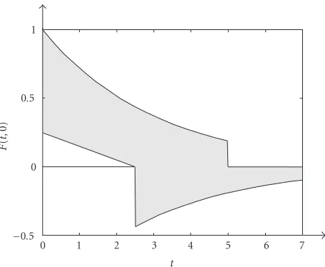
Figure 3.1. Graph of the multifunctiont→F(t, 0).

Lemma3.1. LetH:X×[0, 1]F be a suitable homotopy such thatH(X, 0)⊂X. Then

H(·, 1)has a fixed point inX.

In applications, the strength of this principle is seldom used, we are thus going to present an example that fully uses the strength of the above lemma. Consider the inclu-sion

u(t)∈Ft,u(t) (3.1)

fort∈[0,∞) with initial conditionu(0)=0. We will look for a solution which satisfies inclusion (3.1) almost everywhere onR+_{in spaceACloc(R}+_{) of all real valued functions} locally absolutely continuous on [0,∞). This space is again endowed with the topology of uniform convergence on compact subintervals. In this particular case, we will look for bounded solutions which “go around” an obstacleO:=[0, 1/10] which is placed att=1.

Let us consider particular right-hand side of inclusion (3.1):

F(t,y) :=

⎧ ⎪ ⎪ ⎪ ⎪ ⎪ ⎪ ⎪ ⎨ ⎪ ⎪ ⎪ ⎪ ⎪ ⎪ ⎪ ⎩

₁

4−

t

10,e

−t/3₊1 3y

for 0≤t≤5

2,

−e−t/3₋1 3y,e−

t/3₊1 3y

for5

2≤t≤5,

−e−t/3₋1 3y, 0

for 5≤t.

(3.2)

Figure 3.1shows the graph of the multifunctiont→F(t, 0).

In order to prove the existence of an entirely bounded solution to (3.1) which goes around the obstacle, we again employ the linearization technique. We define the param-eter set

and the obstacle set

Q:=q∈Q;q(1) ∈O, (3.4)

whereO=[0, 1/10]. With respect to the first section, we see thatQis closed and convex subset of the Fr´echet spaceACloc(R+_{) andQis its relatively open subset. It is easy to}

ver-ify, that the relative boundary∂QQofQwith respect toQis formed by those functions

q∈Qthat satisfyq(1)=0 orq(1)=1/10.

Let us now define a homotopy H: [0, 1]×QACloc(R+_{) which to any (λ,q)∈} [0, 1]×Qassociates all solutions to

u(t)∈Ft,λq(t), (3.5)

whereF is given by (3.2) and boundary conditions of (3.1) remain valid. We want to applyLemma 3.1and show thatH(1,·) has a fixed point inQwhich corresponds to the desired solution to the original problem. In order to draw such conclusion we need to show that

(1)His compact,

(2)His upper semi-continuous with compact and convex values, (3)Hdoes not have any fixed points on the relative boundary∂QQ, (4)H(0,Q)⊂Q.

ad 1. We need to prove thatH([0, 1]×Q) is a relatively compact subset ofACloc(R+_). In view ofProposition 2.1, it is sufficient to prove thatH([0, 1]×Q) is equicontinuous. The estimate|q(t)| ≤3 for allq∈Qand relation (3.2) imply that|F(t,q(t))| ≤2 for all

t∈R+_{. This means that|u(t)| ≤2 for allu∈H([0, 1]×Q). Such uniform boundedness}

ofuimplies equicontinuity ofH([0, 1]×Q). This proves the compactness of homotopy

H.

ad 2. SinceH is compact, it is sufficient to prove thatH has closed graph in order to conclude that it is upper semi-continuous. (See [3, Section I, Proposition 3.16].) Let us take a sequence (λn,qn,un) in the graph ofHwhich converges to (λ,q,u) in [0, 1]×Q×

ACloc(R+_{). We want to show thatu∈H(λ,q), which means thatusatisfies (3.5) for} al-most allt∈R+_{. Let us fixt}

0∈R+such thatun(t0) andu(t0) exist. Note that the

comple-ment of the set of all sucht0∈R+has zero measure due to the local absolute continuity ofunandu. We know that

unt0

∈Ft0,λnqnt0

, (3.6)

which together with the closedness of the values ofFimplies

ut0

∈lim

n→∞F

t0,λnqnt0

. (3.7)

The continuity of the mappingy→F(t0,y), which is clear from (3.2), implies that

lim

n→∞F

t0,λnqnt0

=Ft0,λqt0

which completes the proof of the upper semi-continuity ofH. SinceH is compact and the graph ofH is closed, we conclude thatH has compact values. The convexity of the values ofH follows from the convexity of the values ofF. Note that compact and convex sets are, in particular,Rδsets. (See [3, Chapter I.2].)

ad 3. Observe that∂QQconsists of such functionsq∈Qthat satisfyq(1)=0 orq(1)=

1/10. Let us suppose there exists such (λ,q)∈[0, 1]×Qthat the solutionuof (3.5) sat-isfiesu(1)=1/10. By the mean value theorem, this implies the existence oft0∈[0, 1] such thatu(t0)≤1/10 which is a contradiction to the form ofFgiven by (3.2). Note that 1/4−t/10>1/10 for allt∈[0, 1]. By the same argument we exclude the possibility that

u(1)=0. This proves the nonexistence of fixed points on the relative boundary ofQ. ad 4. At last we show that H(0,Q)⊂Q. By an analogous argument to the previous paragraph, we can show thatu(1) ∈Ofor all u∈H(0,Q). The particular form ofF

implies that allu∈H(0,Q) have to be nondecreasing on [0, 5/2] and nonincreasing on [5,∞). Simple calculation shows that |u(t)| ≤3 for allt∈R+_{andu∈H(0,Q) which}

completes the argument.

We have shown that all the assumption of Lemma 3.1are satisfied and we can there-fore establish the existence of a fixed point ofH(1,·) which represents an entirely bounded solution to (3.1) which goes around the given obstacle.

4. Application to partial differential inclusions

In this section we present a possible extension of the continuation principle which shows the possibility of application of such principles in solving partial differential inclusions in Banach spaces.

Let us first introduce the Bochner spaceWp,q_{(K,V1,V2), whereK is a compact}

in-terval,V1andV2Banach spaces. The spaceWp,q(K,V1,V2) consists of functionsusuch that

(i)u(t)∈V1for anyt∈K, (ii)u∈Lp_{(K,V1) in the sense that}

Ku(t) p

V1dtis finite, (iii) (du/dt)(t)∈V2for anyt∈K,

(iv)du/dt∈Lq_{(K,V2) in the sense that}

K(du/dt)(t) q

V2dtis finite,

where the derivatives are understood in the weak sense. IfK is a compact interval then

Wp,q_{(K,V1,V2), endowed with the norm}

uWp,q:= u_Lp_(K,V1)+ du_dt

Lq_(K,V2)

=

K

_u(t)p V1dt

1/ p

+

K

du_dt(t)

q

V2

dt

1/q

,

(4.1)

becomes a Banach space.

the seminorm

pk(v) := vWp,q_(K

k,V1,V2). (4.2)

Then the spaceWp,q_{(I,V1,V2) equipped with the metric}

du1,u2

:=

j∈N

1 2j

pj

u1−u2

1 +pj

u1−u2

(4.3)

becomes a complete metric space. Consider the inclusion

du

dt(t) +Au(t)∈F

t,u(t), (4.4)

wheret∈Ian arbitrary interval. Inclusion (4.4) has an abstract boundary condition

u∈S⊂Wp,q_I,V1,V

2

. (4.5)

LetA:V1→V2be an operator (not necessarily linear), the properties of which are to be specified later. This operator represents the “spacial” part of the inclusion and in ap-plications it usually stands for a differential operator of the second order from the Banach spaceV into its dualV∗. Exponents pandqare usually dual and their qualification is given inLemma 4.1. LetF:I×V1V2be a multivalued map and letSbe a nonempty subset ofWp,q_(I,V1,V2).

By astrong solutionto problem (4.4) with boundary condition (4.5) we understand a functionu∈Wp,q_{(I,V1,V2) which satisfies boundary condition (4.5) and satisfies}

inclu-sion (4.4) onV2for almost allt∈I.

First, we are going to prove a technical lemma, which will be used later and which provides the qualification of the right-hand side of inclusion (4.4). We will need these definitions.

LetF:I×V1V2be a multivalued map. For (t,v)∈I×V1we define _F(t,v)

V2:=sup

fV2:f ∈F(t,v)

. (4.6)

LetF:I×V1V2be a multivalued map. We define theNemyckii operatorNF:Lp(I,V1) Lq_{(I,V2) by}

NF(v) :=f ∈LqI,V2

:f(t)∈Ft,v(t)for almost allt∈I. (4.7)

The following lemma justifies the above definition and describes the properties of the Nemyckii operator.

Lemma4.1. LetK be a compact interval, p,q≥1,V1V2 continuously and letF:K×

V1V2satisfy conditions

(iii)F(t,v) :K×V1V2is product measurable, (iv)F(t,v)V2≤α(t) +βv

p/q

V1, whereα∈L

q_{(K)andβ≥0,}

then the Nemyckii operatorNF:Lp(K,V1)Lq(K,V2)has nonempty, closed and convex

values and is upper semi-continuous. Moreover, it satisfies the following property:

un−→uinWp,qI,V1,V2

fn∈NFun, fn f weakly inLqK,V2

implies that f ∈NF(u). (4.8)

Proof. The proof of the first part of the statement follows directly from [8, page 237]. For p,q≥1 andV1V2it holds thatWp,q(K,V1,V2)C(K,V2). (See [7, page 173].) The proof of part two now follows from [1] (see [1, Lemma 14]) and from the obvious

embeddingLq_(K)L1_{(K), forq≥1.}

We now specify the properties of the operatorA. LetAbe locally bounded in the sense that

AvV2≤C

1 +vp/qV1

(4.9)

for anyv∈V1. Observe that foru∈Lp_{(K,V1) we then have}

K

_Au(t)q V2dt≤

KC

q_{1 +u(t)}p/q V1

q

≤M

K

_u(t)p

V1, (4.10)

which is finite becauseu∈Lp_{(K,V1). We further define operatorᏭby}

(Ꮽu)(t) :=Au(t). (4.11)

IfAis bounded in the sense of (4.9), then the above calculation shows thatᏭ:Lp_(K, V1)→Lq_(K,V2).

We will further need some notion of continuity ofᏭ. The following definition turns out to be optimal.

Operator Ꮽ:Lp_(I,V1)→Lq_{(I,V2) isdemicontinuous ifun→uin L}p_{(I,V1) implies}

Ꮽ(un)Ꮽ(u) weakly inLq_{(I,V2). OperatorᏭislocally demicontinuousif it is}

demi-continuous for anyK⊂Icompact.

We now want to employ the standard technique of partial linearization of the right-hand side of inclusion (4.4). We need to prove that the solution operator of the linearized problem has closed graph. This, together with some compactness argument, will guaran-tee the upper semi-continuity of the solution operator.

Lemma4.2. LetG:I×V1×V1V2satisfy assumptions (i)–(iv) ofLemma 4.1jointly in

V1×V1. LetSbe a nonempty and closed subset ofWp,q(I,V1,V2). LetAbe bounded in the sense of (4.9) and letᏭdefined in (4.11) be locally demicontinuous. Let there exist a closed

Q⊂Wp,q_{(I,V1,V2)such that for anyq∈Qthe problem} du

dt(t) +Au(t)∈G

t,u(t),q(t), u∈S, (4.12)

Proof. Choose (qn,un) an arbitrary sequence in the graph ofTsuch that (qn,un)→(q0,u0) inWp,q_(I,V1,V2)×Wp,q_{(I,V1,V2). SinceSis closed, we haveu}

0∈S. We need to show thatu0∈T(q0) which means that

du0

dt (t) +Au0(t)∈G

t,u0(t),q0(t) (4.13)

for almost allt∈I. We know that

dun

dt (t) +Aun(t)∈G

t,un(t),qn(t)

. (4.14)

Let us confine to anyK⊂Icompact. In view ofLemma 4.1, it is sufficient to show that

dun dt +Ꮽ

un

du0

dt +Ꮽ

u0

weakly inLq_K,V

2

. (4.15)

The convergencedun/dt→du0/dt inLq(K,V2) is ensured by the first step of the proof and the weak convergenceᏭ(un)Ꮽ(u0) follows from the demicontinuity ofᏭ. This

proves (4.15) and in view ofLemma 4.1indeed (4.13) holds for almost allt∈K. SinceK

is arbitrary, we conclude that (4.13) holds for almost allt∈I, which meansu0∈T(q0). We are now in the position to prove the main result of this section—the continuation principle. We again consider problem (4.4) with boundary condition (4.5).

Proposition4.3. LetG:I×V1×V1×[0, 1]V2satisfy the assumptions ofLemma 4.1 jointly inV1×V1and uniformly on[0, 1]. LetG(t,c,c, 1)⊂F(t,c)for all(t,c)∈I×V1. Let Abe locally bounded in the sense of (4.9) andᏭlocally demicontinuous. LetS⊂Wp,q_(I,V1, V2)be nonempty and closed. Let there exist a closed convexQ⊂Wp,q_{(I,V1,V2)such that}

for any(s,q)∈[0, 1]×Qthe problem

du

dt(t) +Au(t)∈G

t,u(t),q(t),s, u∈S, (4.16)

has a solution such that the solution operatorT: [0, 1]×QShas the following properties: (i)for any(s,q)∈[0, 1]×Q, setT(s,q)isRδ,

(ii)Tis compact, (iii)T(Q, 0)⊂Q,

(iv)for any fixed pointq∈T(s,q), there exists a neighborhoodᐁqinQsuch thatT([0,

1]×ᐁq)⊂Q.

Then problem (4.4) together with boundary condition (4.5) has a solution.

u∈T(u, 1) which is a solution to the inclusion

du

dt(t) +Au(t)∈G

t,u(t),u(t), 1, u∈S. (4.17)

RelationG(t,c,c, 1)⊂F(t,c) ensures that this fixed pointuis a solution to the original

problem.

5. Illustrating example

As an example we will consider inclusion

du

dt −Δu∈F(t,u), u∈S, (5.1)

wheret∈I an arbitrary interval andx∈Ωa bounded subset ofRn_{and the properties}

ofFandSare to be specified later. We will look for a strong solution to problem (5.1) in spaceW2,2_(I,W1,2_(Ω),L2_{(Ω)). For the sake of simplicity, we denote}

W2,2_:=W2,2_I,W1,2_(Ω),L2_(Ω), L2L:=L2

I,L2_(Ω). (5.2)

We will now specifySas follows:

S:=u∈W2,2_{:u(0)=u0,u=0∀(t,x)∈I×∂Ω. (5.3)}

Note that this definition has meaning, because the functions involved have continuous representants.

Let the right-hand sideF:I×L2_(Ω)L2_{(Ω) satisfy the following assumptions:} (i)F(t,v) is nonempty, closed and convex for all (t,v)∈I×L2_(Ω),

(ii)Fis product measurable, (iii)F(t,·) is upper semi-continuous,

(iv)|F(t,v)| ≤α(t) +βvL2, whereα∈L2(I) andβ <1/2.

It follows fromLemma 4.1, thatNF:L2LL2Lis upper semi-continuous with nonempty,

closed and convex values.

Let us now define the linearization set

Q:=q∈W2,2:q(t)_L2≤M∀t∈I

, (5.4)

whereMis to be specified later. Takeq∈Qarbitrary. The obvious embeddingW2,2_L2 L

gives a nonempty, closed and convexNF(q)⊂L2

L. For arbitrary f ∈NF(q) we will solve

the linearized problem

du

dt −Δu= f(t), u∈S. (5.5)

It is well-known that problem (5.5) has a unique strong solutionu∈W2,2_{. (See [5,}

Chap-ter 7, Theorem 5].) Moreover, the solution operatorK:L2

L→W2,2such thatK f =uis

first prove thatu∈Q. We need to show thatu(t)L2≤M. Multiplying (5.5) byu, inte-grating overΩand integrating from 0 tot, we obtain

t

0

Ω

du dtu−

t

0

Ω(Δu)u= t

0

Ωf u. (5.6)

Applying the Green theorem and rearranging the terms we obtain t

0 1 2

d dtu

2

L2− t

0

∂Ω ∂u ∂νu+

t

0

Ω∇u· ∇u= t

0

Ωf u. (5.7)

Sinceu∈S, the boundary integral equals to zero. We apply the H¨older and Young in-equalities to the right hand-side and obtain

1 2u(t)

2

L2− 1 2u0

2

L2+ t

0∇u 2

L2≤C1 t

0f 2

L2+ 1 2

t

0u 2

L2, (5.8)

such thatC1<2. Sinceu=0 on∂Ω, we employ the Poincar´e inequality to obtain

1 2u(t)

2

L2+B _t

0u 2

W1,2≤C1 _t

0f 2

L2+ 1 2u0

2

L2. (5.9)

Using the properties ofFand the definition ofQ, we obtain t

0f 2

L2≤ t

0α

2_+β2_M≤C

2+β2M, (5.10)

which substituted back to (5.9) gives

1 2u(t)

2

L2≤C3+C1β2M. (5.11)

SinceC3>0,C1<2,β2<1/4, it is possible to setM, such that

C3+C1β2M≤M

2. (5.12)

Indeed, it is sufficient to take

M:= 2C3 1−2C1β2

. (5.13)

This shows that any solutionuto problem (5.5) satisfiesu∈S. Altogether, we have the following sequence of mappings:

q∈Q⊂W2,2_−→q∈L2

LNF(q)⊂L2L−→K

NF(q)

⊂Q⊂W2,2_{, (5.14)}

where the first mapping is the compact inclusionW2,2_L2

L, the second one is the

thatT has a fixed point, we need to ensure thatT is compact or, at least, condensing with respect to a suitable measure of noncompactness. Due to the compactness of the first inclusion, it is sufficient thatNFmaps compact sets on compact (or at least

precom-pact) sets. Let us mention that this condition is satisfied for example, ifFis single valued (then the single valued Nemyckii map becomes continuous), or ifNF(q) consists of finite number of points (compare [9]).

Acknowledgment

The author would like to thank Professor Jan Andres for bringing up the topic, for fruitful discussions on the theme, and for numerous inspirating consultations.

References

[1] J. Andres and R. Bader,Asymptotic boundary value problems in Banach spaces, Journal of Math-ematical Analysis and Applications274(2002), no. 1, 437–457.

[2] J. Andres, G. Gabor, and L. G ´orniewicz,Boundary value problems on infinite intervals, Transac-tions of the American Mathematical Society351(1999), no. 12, 4861–4903.

[3] J. Andres and L. G ´orniewicz, Topological Fixed Point Principles for Boundary Value Problems, Topological Fixed Point Theory and Its Applications, vol. 1, Kluwer Academic, Dordrecht, 2003. [4] K. Borsuk,Theory of Retracts, Monografie Matematyczne, vol. 44, Pa ´nstwowe Wydawnictwo

Naukowe, Warsaw, 1967.

[5] L. C. Evans,Partial Differential Equations, Graduate Studies in Mathematics, vol. 19, American Mathematical Society, Rhode Island, 1998.

[6] M. Furi and M. P. Pera,On the fixed point index in locally convex spaces, Proceedings of the Royal Society of Edinburgh. Section A. Mathematics106(1987), no. 1-2, 161–168.

[7] H. Gajewski, K. Gr¨oger, and K. Zacharias,Nichtlineare Operatorgleichungen und Operatordiffer-entialgleichungen, Mathematische Lehrb¨ucher und Monographien, II. Abteilung, Mathematis-che Monographien, vol. 38, Akademie, Berlin, 1974.

[8] S. Hu and N. S. Papageorgiou,Handbook of Multivalued Analysis. Vol. I. Theory, Mathematics and Its Applications, vol. 419, Kluwer Academic, Dordrecht, 1997.

[9] A. Margheri and P. Zecca,Solution sets and boundary value problems in Banach spaces, Topolog-ical Methods in Nonlinear Analysis2(1993), no. 1, 179–188.

[10] H. H. Schaefer,Topological Vector Spaces, The Macmillan, New York; Collier-Macmillan, Lon-don, 1966.

Tom´aˇs F¨urst: Department of Mathematical Analysis and Applications of Mathematics, Faculty of Science, Palack´y University, Tomkova 40, 779 00 Olomouc, Czech Republic