R E S E A R C H
Open Access
An operator method for telegraph partial
differential and difference equations
Allaberen Ashyralyev
1*and Mahmut Modanli
2*Correspondence:
1Department of Mathematics, Fatih
University, Istanbul, 34500, Turkey Full list of author information is available at the end of the article
Abstract
The Cauchy problem for abstract telegraph equations d2dtu2(t)+
α
dudt(t)+Au(t) +β
u(t) = f(t) (0≤t≤T),u(0) =ϕ
,u(0) =ψ
in a Hilbert spaceHwith the self-adjoint positive definite operatorAis studied. Stability estimates for the solution of this problem are established. The first and second order of accuracy difference schemes for the approximate solution of this problem are presented. Stability estimates for the solution of these difference schemes are established. In applications, two mixed problems for telegraph partial differential equations are investigated. The methods are illustrated by numerical examples.Keywords: telegraph equations; Cauchy problem; Hilbert space; difference schemes; stability
1 Introduction
Hyperbolic partial differential equations arise in many branches of science and engineer-ing,e.g., electromagnetic, electrodynamics, thermodynamics, hydrodynamics, elasticity, fluid dynamics, wave propagation, materials science. In numerical methods for solving these equations, the problem of stability has received a great deal of importance and at-tention. Specially, a suitable model for analyzing the stability is provided by a proper un-conditionally absolutely stable difference scheme with an unbounded operator. The role played by the positivity property of differential and difference operators in Hilbert and Banach spaces in the study of various properties of boundary value problems for partial differential equations, of stability of difference schemes for partial differential equations, and of summation Fourier series is well known (see [–]).
The method of operators as a tool for the investigation of the solution of local and non-local problems to hyperbolic differential equations in Hilbert and Banach spaces, has been systematically developed by several authors (see,e.g., [–, , ]).
The telegraph hyperbolic partial differential equation is important for modeling several relevant problems such as signal analysis, wave propagation, random walk theory [–]. To deal with the equation, various mathematical methods have been proposed for ob-taining exact and approximate analytic solutions. For instances, Dehghan and Shokri pro-posed a new numerical scheme based on radial based function method (Kansa’s method) []. Gao and Chi developed a numerical algorithm for the solution of nonlinear tele-graph equations []. Biazaret al.applied the variational iteration method to obtain an ap-proximate of the telegraph equations []. Saadatmandi and Dehghan used the Chebyshev
tau method in numerically solving the telegraph equation []. Koksal computed numer-ical solutions the telegraph equations arising in transmission lines []. Twizell used the explicit difference method for the wave equation with extended stability range []. Fi-nally, Ashyralyev and Akat applied the difference method for the approximate solution of stochastic hyperbolic and stochastic telegraph equations [–].
In the present paper, we consider a Cauchy problem for telegraph equations
du(t)
dt +α
du(t)
dt +Au(t) +βu(t) =f(t) (≤t≤T),
u() =ϕ, u() =ψ ()
in a Hilbert spaceHwith a self-adjoint positive definite operatorAandA≥δI. Hereδ> ,
α> and
β+δ≥α
. ()
A function u(t) is called a solution of the problem () if the following conditions are satisfied:
i. u(t)is twice continuously differentiable on the segment[,T]. The derivatives at the endpoints of the segment are understood as the appropriate unilateral derivatives. ii. The elementu(t)belongs toD(A)for allt∈[,T]and the functionAu(t)is
continuous on the segment[,T].
iii. u(t)satisfies the equation and initial conditions ().
The paper is organized as follows. Section is an introduction where we provide the definition of the solution of the Cauchy problem (). In Section , stability estimates for the solution of this problem are established. In applications, two mixed problems for tele-graph partial differential equations are investigated. In Section , the difference schemes of the first and second order of accuracy for the approximate solution of problem () are presented. Stability estimates for the solution of these difference schemes are estab-lished. In applications, stability estimates for the solution of difference schemes for the two mixed problems for telegraph partial differential equations are established. In Section , the methods are illustrated by numerical examples. Section is for our conclusion.
2 The main theorem on stability
Let{c(t),t≥}be a strongly continuous cosine operator-function defined by the formula
c(t) = e
itB/+e–itB/
.
Then, from the definition of the sine operator-functions(t),
s(t)u=
t
c(s)u ds
it follows that
s(t) =B–/e
itB/–e–itB/
HereB=A+ (β–α)I. It is easy to check under the assumption () that the problem () for a telegraph equation has a unique mild solution given by the formula
u(t) =e–αtc(t)ϕ+α
e
–αts(t)ϕ+e–αts(t)ψ+
t
e–α(t–z)s(t–z)f(z)dz. ()
In fact, explicitly () can be rewritten as the equivalent initial-value problem for a system of first-order differential equations
⎧ ⎪ ⎨ ⎪ ⎩
u(t) +αv(t) +iBu(t) =z(t) (≤t≤T),
u() =u, u() =u, z(t) +αz(t) –iBz(t) =f(t).
()
Integrating these, now we get
⎧ ⎪ ⎨ ⎪ ⎩
u(t) =e–(α+iB)tu() +t
e–
(α +iB
)(t–s)
z(s)ds,
z(t) =e–(α–iB
)tz() +t
e –(α –iB
)(t–s)
f(s)ds.
Applying the initial conditionz() =u() + (α+iB)u(), we get
u(t) =e–(α+iB )tu() +
t
e–(
α +iB
)(t–s) s
e–(
α –iB
)(s–p)
f(p)dp ds
+
t
e–(
α +iB
)(t–s)
e–(α–iB )s
ds u() + α +iB
u()
.
By an interchange of the order of integration, we can write
u(t) =
e–(α+iB )t+ α
+iB
t
e–(
α +iB
)(t–s)
e–(α–iB )sds
u()
+
t
e–(α+iB
)(t–s)e–(α–iB)sds u()
+
t
e–α(t–s)B–e
i(t–s)B
–e–i(t–s)B
i f(s)ds
=e–αt
eitB
+e–itB
+
α
B –etiB
–e–itB
i
u()
+e–αt
B–e
itB
–e–itB
i
u()
+
t
e–α(t–s)B–e
i(t–s)B
–e–i(t–s)B
i f(s)ds.
Thus, by the definitions ofB,c(t), ands(t) we obtain (). We will prove the following
Theorem . Suppose thatϕ∈D(A),ψ∈D(A)and f(t)is a continuously differentiable
function on[,T]and the assumption()holds.Then there is a unique solution of problem ()and the stability inequalities
max
≤t≤T
u(t)H≤M
ϕH+A–/ψH+ max
≤t≤T
A–/f(t)H
, ()
max
≤t≤T
dudt(t)
H
+ max
≤t≤T
A/u(t)H
≤MA/ϕH+ψH+ max
≤t≤T
f(t)H
, ()
max
≤t≤T
ddtu(t)
H
+ max
≤t≤T
Au(t)H
≤M
AϕH+A/ψH+f()H+ max
≤t≤T
f(t)H
()
hold,where M does not depend onϕ,ψ,and f(t).
Proof Using (),A≥δI, and the following estimates:
c(t)H→H≤, B
s(t)H→H≤, |e–αt| ≤, B–/ϕ
H≤√δϕH, A/B–
H→H≤M(δ), ()
we can write the following inequalities:
u(t)H≤c(t)H→He–αtϕH+Bs(t)
H→HA
/B–
H→H,
eαα
t
A–/ϕH+Bs(t)
H→HA
/B–
H→He
–αtA–/ψ
H
+
t
Bs(t–s)
H→HA
/B–
H→HA
–/f(s)
Hds
≤M(δ)
ϕH+A–/ψH+ max
≤t≤T
A–/f(t)H
for anyt∈[,T]. Then we obtain
max
≤t≤T
u(t)H≤M(δ)
ϕH+A–/ψH+ max
≤t≤T
A–/f(t)H
.
ApplyingA to () and using the estimate for (), in a similar manner, we get
Au(t)
H≤c(t)H→He
–α
tAϕ
H
+Bs(t)
H→HA
/B–
H→H
eαα
t
ϕH
+Bs(t)
H→HA
/B–
H→He
–αtψ H
+
t
A/B–
H→HB
s(t–s)
H→Hf(s)Hds
≤M(δ)
Aϕ
H+ψH+max≤t≤Tf(t)H
for anyt∈[,T]. Then we get
max
≤t≤T
Au(t)
H≤M(δ)
Aϕ
H+ψH+max≤t≤Tf(t)H
.
Now, we obtain an estimate forAu(t)H. ApplyingAto () and using an integration by
parts, we can write the formula
Au(t)eαt=c(t)Aϕ+α
A
s(t)Aϕ+As(t)Aψ
+AB–
f(T) –c(t)f() –
t
c(t–s)f(s)ds
.
Using the last formula and estimates (), we obtain
Au(t)H≤c(t)H→He–αtAϕH
+Bs(t)
H→HA
/B–
H→H
eαα
t
Aϕ
H
+Bs(t)
H→HA
/B–
H→He
–αtAψ H
+AB–H→Hf(T)H+c(t)H→Hf()H +AB–H→H
t
c(t–s)H→Hf(s)Hds
≤M(δ)
AϕH+A
ψ
H+f()H+max≤t≤Tf
(t)
H
for anyt∈[,T]. Then we get
max
≤t≤T
Au(t)H≤M(δ)
AϕH+A
ψ
H+f()H+max≤t≤Tf
(t)
H
.
The estimate formax≤t≤Td
u
dtHfollows from the last estimate and the triangle
inequal-ity. Theorem .. is proved.
Remark . All statements of Theorem . hold in an arbitrary Banach spaceEunder the assumptions (see,e.g., [, ]):
c(t)E→E≤M, B
s(t)E→E≤M, B–/ϕ
E≤M(δ)ϕE, A/B–
E→E≤M(δ). ()
Now, we consider the application of this abstract theorem, Theorem .. First, we con-sider the initial-value problem for the telegraph equations
⎧ ⎪ ⎪ ⎪ ⎨ ⎪ ⎪ ⎪ ⎩
utt(t,x) +αut(t,x) – (a(x)ux)x+δu(t,x) +βu(t,x)
=f(t,x), <t<T, <x<l,
u(,x) =ϕ(x), ut(,x) =ψ(x), ≤x≤l,
u(t, ) =u(t,l), ux(t, ) =ux(t,l), ≤t≤T.
()
us to reduce the problem () to the initial value () in a Hilbert spaceH=L[,l] with a self-adjoint positive definite operatorAxdefined by (). Let us give a number corollaries
of the abstract Theorem ..
Theorem . For solutions of the problem()the stability inequalities
max
≤t≤T
u(t,·)W
[,l]≤M
max
≤t≤T
f(t,·)L
[,l]+ϕW[,l]+ψL[,l]
, ()
max
≤t≤T
u(t,·)W [,l]+
max
≤t≤T
utt(t,·)L[,l]
≤M
max
≤t≤T
ft(t,·)L
[,l]+f(,·)L[,l]+ϕW[,l]+ψW[,l]
()
hold,where Mdoes not depend on f(t,x)andϕ(x),ψ(x).
Proof Problem () can be written in abstract form
du(t)
dt +αdudt(t)+Au(t) +βu(t) =f(t) (≤t≤T),
u() =ϕ, u() =ψ ()
in a Hilbert space L[,l] of all square integrable functions defined on [,l] with self-adjoint positive definite operatorA=Axby the formula
Axu(x) = –a(x)ux
x+σu(x) ()
with the domain
DAx=u(x) :u,ux,
a(x)ux
x∈L[,l],u() =u(l),u
() =u(l).
Here,f(t) =f(t,x) andu(t) =u(t,x) are known and unknown abstract functions defined on [,l] with the values inH=L[,l]. Therefore, estimates () and () follow from es-timates (), (), and (). Thus, Theorem . is proved.
Second, let⊂Rnbe a bounded open domain with smooth boundaryS,=∪S. In
[,T]×we consider the boundary value problem for telegraph equations
⎧ ⎪ ⎪ ⎪ ⎨ ⎪ ⎪ ⎪ ⎩
utt(t,x) +αut(t,x) –
n
r=(ar(x)uxr)xr+βu(t,x) =f(t,x), x= (x, . . . ,xn)∈, <t<T,
u(,x) =ϕ(x), ∂u(,∂tx)=ψ(x), x∈, u(t,x) = , x∈S, ≤t≤T,
()
where ar(x) (x∈),ϕ(x),ψ(x) (x∈) andf(t,x), t∈(,T), x∈, are given smooth
functions andar(x) > . We introduce the Hilbert spaceL(), the space of all integrable functions defined on, equipped with the norm
fL()=
· · ·
x∈
f(x)dx· · ·dxn
Theorem . For solutions of the problem()the stability inequalities
max
≤t≤T
u(t,·)W ()≤M
max
≤t≤T
f(t,·)L
()+ϕW()+ψL()
, ()
max
≤t≤T
u(t,·)W
()+max≤t≤T
utt(t,·)L()
≤M
max
≤t≤Tft(t,·)L()+f(,·)L()+ϕW()+ψW()
()
hold,where Mdoes not depend on f(t,x)andϕ(x),ψ(x).
Proof Problem () can be written in the abstract form () in Hilbert spaceL() with self-adjoint positive definite operatorA=Axdefined by formula
Axu(x) = –
n
r=
ar(x)uxr
xr+σu(x) () with domain
DAx=u(x) :u(x),uxr(x),
ar(x)uxr
xr∈L(), ≤r≤n,u(x) = ,x∈S
.
Here,f(t) =f(t,x) andu(t) =u(t,x) are known and unknown abstract functions defined onwith the values inH=L(). So, estimates () and () follow from estimates (),
(), and () and the following theorem.
Theorem . For the solutions of the elliptic differential problem[]
⎧ ⎨ ⎩
Axu(x) =ω(x), x∈,
u(x) = , x∈S,
the following coercivity inequality holds:
n
r=
uxrxrL()≤MωL().
Here Mdoes not depend onω(x).
In Section , the difference schemes of the first and second order of accuracy for the approximate solution of problem () are investigated. Stability estimates for the solution of these difference schemes are established. In applications, difference schemes for the approximate solution of the two mixed problems () and () are presented. Stability estimates for the solution of these difference schemes are established.
3 Stability of two-step difference schemes
First, we consider the approximation of first order intof the two-step difference scheme for the numerical solution of the initial value problem ()
⎧ ⎪ ⎨ ⎪ ⎩
uk+–uk+uk–
τ +α
uk+–uk–
τ +Auk++βuk+=fk, fk=f(tk+), ≤k≤N– ,Nτ=T,
u=ϕ, uτ–u+ (A+ (β–α
)I)τu= +ατψ.
Now, we will consider operatorsR,Rdefined by
R= I+i –ατ
+ατ
I+τ B+α I –I P,
R= I–i –ατ
+ατ
I+τ B+α I –I P, P=
+ατ
I+τ B+α
I
–
,
and we will introduce the following operators:
R=
ατ+τ
B
+ ατ
+iτB/ +ατ+τB+α τ
– ατ–α τ B – ×
–iτB/
– ατ–α τ
B
– +ατ+τB+ατ
–
,
R= τ
+B+α τ
+
ατ B
– +ατ+ τB+ατ
× –iB +ατ+τB+α
τ
– ατ–α τ
B –
– ,
R= τB
+ατ+ τB+α
τ
×
+ατ+τB+α τ
iτB
– ατ–α τ
B –
–
,
R= + τB– ατB–
ατ
×
–iB
– ατ–α τ
B –
× +ατ+ τB+α τ
( –ατ)
– ,
R= –ατ– τB–
ατ
+iτB
– ατ–α τ B – ×
+ατ+ τB+α τ
–
,
R= –iτB
– ατ–α τ
B –
× ατ+ τB+α τ
–iτB
– ατ–α τ B – – , ()
Lemma . The following estimates hold:
⎧ ⎪ ⎪ ⎪ ⎪ ⎪ ⎪ ⎪ ⎪ ⎨ ⎪ ⎪ ⎪ ⎪ ⎪ ⎪ ⎪ ⎪ ⎩
RH→H≤, RH→H≤,
RH→H≤, RH→H≤,
B/RH→H≤, τB/RH→H≤,
B/R
H→H≤, B–/RH→H≤τ,
B–/R
H→H≤τ,
τB/R
H→H≤, τB/RH→H≤.
()
Theorem . Suppose that the assumption()holds andϕ∈D(A),ψ∈D(A).Then for
the solution of difference scheme()the stability estimates
max
≤k≤NukH≤M
max
≤k≤N–
A–/fkH+A–/ψH+ϕH
, ()
max
≤k≤N
A/ukH≤M
max
≤k≤N–fkH+ψH+
A/ϕH
, ()
max
≤k≤NAukH≤M
max
≤k≤N–
τ(fk–fk–)
H
+fH+A/ψH+AϕH
()
hold,where M does not depend onτ,ϕ,ψ,and fk, ≤s≤N– .
Proof We will obtain the formula for the solution of the problem (). We can rewrite () into the following difference problem:
⎧ ⎪ ⎨ ⎪ ⎩
( –ατ )Iuk–– Iuk+ (( +ατ )I+τ(B+α
I))uk+ =τfk, ≤k≤N– ,
u=ϕ, u= (I+Bτ)–ϕ+τ( +ατ )–(I+Bτ)–ψ.
()
It is clear that there exists a unique solution of this initial-value problem and for the solu-tion of (), the following formula is satisfied (see []):
u=ϕ, u=
I+Bτ–ϕ+τ +ατ
–
I+Bτ–ψ,
uk=RR(R–R)–
Rk––Rk–ϕ
+ (R–R)–Rk–RkI+Bτ–ϕ+τ +ατ
–
I+Bτ–ψ
+
k–
s=
RR (R–R) –ατ
–
Rk–s–Rk–sτfs.
()
Using the spectral property of the self-adjoint positive definite operators, we get
I+Bτ–H→H≤,
τBI+Bτ–
H→H≤, τ
BI+Bτ–
H→H≤.
Then, using the triangle inequality, we get
uH≤I+Bτ
–
H→HϕH
+ +ατ
–
AB–
H→HτB
I+Bτ–
H→HA
–/ψ
H
≤A–/ψH+ϕH. ()
In exactly the same manner, one establishes
Au
H≤I+Bτ
–
H→HA
ϕ
H
+ +ατ
–
AB–
H→HτB
I+Bτ–
H→HψH
≤ ψH+A
ϕ
H, ()
AuH≤I+Bτ
–
H→HAϕH
+ +ατ
–
AB–
H→HτB
I+Bτ–
H→HψH
≤Aψ
H+AϕH. ()
Using the spectral property of the self-adjoint positive definite operators, we get
RH→H≤, τB
R
H→H≤, τ
BR
H→H≤, ()
RH→H≤, τB
R
H→H≤, τ
BR
H→H≤. ()
Now, we will establish estimates forukH,k≥. Using (), the estimates for (), (),
(), (), and the triangle inequality, we get
ukH≤
RH→HRkH→H+RH→HRkH→H
ϕH
+ A
/R
H→HRkH→H+A/RH→HRkH→H
×I+Bτ–H→HA–/H→HϕH+τ +
ατ
–
A–/ψ
H
+ τA
/R H→H
N–
s=
Rk–sH→H+Rk–sH→HτA–/fsH
≤M
N–
s=
A–/fsHτ+ϕH+A–/ψH
for anyk≥. Combining the estimates forukfor anyk, we obtain ().
ApplyingA/ to () and using estimates for (), (), (), (), and the triangle in-equality, we get
A/ukH≤
RH→HRkH→H+RH→HRkH→HA/ϕH
+ A
/R
H→HRkH→H+A/RH→HRkH→H
×I+Bτ–
H→H
A–/H→HA/ϕH+τ +ατ
–
ψH
+ τA
/R H→H
N–
s=
Rk–sH→H+Rk–sH→HτfsH
≤M
N–
s=
fsHτ+A/ϕH+ψH
for anyk≥. Combining the estimates forA/u
kfor anyk, we obtain (). Finally,
applying Abel’s formula to (), we can write
uk=
RR
k–R
Rk
ϕ+
R
k–RkR
I+Bτ–ϕ+τ +ατ
–
I+Bτ–ψ
+ R
k–RkR
τf+ τ
R
!k–
s=
RRk–s–RRk–s
(fs–fs–)
+ (R–R)fk––RRk––RRk–
f
"
, ≤k≤N. ()
Next, applyingAto () and using estimates for (), (), (), (), we get
AukH≤
RH→HRkH→H+RH→HRkH→H
AϕH
+ A
/R
H→HRkH→H+A/RH→HRkH→H
×I+Bτ–H→HA–/H→HAϕH+τ +
ατ
–
A/ψH
+ τA
/R
H→HRkH→H+τA/RH→HRkH→H
τA/fH
+ τA
/R H→H
N–
s=
τA/RH→HRk–sH→H
+τA/RH→HRk–sH→H
× fs–fs–H+τA/RH→H+τA/RH→H
fk–H
+τA/RH→HRk–H→H+τA/RH→HRk–H→H
fH
≤M
N–
s=
fs–fs–H+fH+AϕH+A/ψH
for anyk≥. Combining the estimates forAukHfor anyk, we obtain (). Theorem .
is proved.
Second, we consider two types of approximations of second order intby two-step dif-ference schemes for the numerical solution of the initial value problem ():
⎧ ⎪ ⎪ ⎪ ⎪ ⎨ ⎪ ⎪ ⎪ ⎪ ⎩
uk+–uk+uk–
τ +α
uk+–uk–
τ +
A
(uk++uk–)
+β(uk++uk–) =fk, fk=f(tk), ≤k≤N– ,
u=ϕ,
u–u
τ +
τ
Bu+ +ατ(
B–
ατB
+
α
I)τu= –ατ
+ατ(ψ+
τ
f), f=f(),
⎧ ⎪ ⎪ ⎪ ⎪ ⎨ ⎪ ⎪ ⎪ ⎪ ⎩
uk+–uk+uk–
τ +α
uk+–uk–
τ +
A
uk+
A
(uk++uk–)
+βuk+β(uk++uk–) =fk, fk=f(tk), ≤k≤N– ,
u=ϕ,
u–u
τ +
τ
Bu+ +ατ(
B–
ατB
+
α
I)τu= –ατ
+ατ(ψ+
τ
f), f=f().
()
Theorem . Suppose that the assumption()holds andϕ∈D(A),ψ∈D(A).Then for
the solution of difference schemes()and()the following stability estimates hold:
max
≤k≤NukH≤M
max
≤k≤N–
A–/f
kH+A–/ψH+ϕH
,
max
≤k≤N
A/ukH≤M
max
≤k≤N–fkH+ψH+
A/ϕH
,
max
≤k≤NAukH≤M
max
≤k≤N–
τ(fk–fk–)
H
+fH+A/ψH+AϕH
hold,where M does not depend onτ,ϕ,ψ,and fk, ≤s≤N– .
The proof of Theorem . is based on the formulas for the solution of the difference schemes () and (), on the estimates for the step operators, and on the self-adjointness and positivity of operatorA.
Now, we consider applications of the main theorem, Theorem .. First, we consider the boundary value problem (). The discretization of problem () is carried out in two steps. In the first step, we define the grid space
[,l]h={x=xn:xn=nh, ≤n≤M,Mh=l}.
Let us introduce the Hilbert spaceLh=L([,l]h) of the grid functionsϕh(x) ={ϕn}M defined on [,l]h, equipped with the norm
ϕhLh=
x∈[,L]h
ϕ(x)h
/ .
To the differential operatorAxdefined by the formula (), we assign the difference
op-eratorAx
hby the formula
Axhϕh(x) =–a(x)ϕx
x,n+δϕn
M–
()
acting in the space of grid functionsϕh(x) ={ϕ
n}M satisfying the conditionsϕ=ϕM,ϕ–
ϕ=ϕM–ϕM–. It is well known thatAxhis a self-adjoint positive definite operator inLh.
With the help ofAxh, we reach the boundary value problem
⎧ ⎪ ⎨ ⎪ ⎩
uh
tt(t,x) +αuht(t,x) +Axhuh(t,x) +βuh(t,x)
=fh(t,x), <t<T,x∈[,l]h,
uh(,x) =ϕh(x), uh
t(,x) =ψh(x), x∈[,l]h.
In the second step, we replace () with the difference scheme (),
⎧ ⎪ ⎪ ⎪ ⎪ ⎪ ⎨ ⎪ ⎪ ⎪ ⎪ ⎪ ⎩
uhk+(x)–uhk(x)+uhk–(x)
τ +α
uhk+(x)–uhk–(x) τ +A
x
huhk+(x) +βukh+(x) =fkh(x),
fh
k(x) =fh(tk+,x),tk=kτ, ≤k≤N– ,x∈[,l]h,Nτ=T,
uh
(x) =ϕh(x),
uh(x)–uh(x)
τ + (A
x h+ (β–
α
)Ih)τu
h
(x) =+ατψ
h(x), x∈[,l] h.
()
Theorem . For the solution{uh
k(x)}N of problem()the following stability estimates:
max
≤k≤N
uhkL
h≤M
max
≤k≤N–
fkhL
h+ψ
h Lh+ϕ
h Lh
,
max
≤k≤N
uhkW h≤M
max
≤k≤N–
fkhL
h+ψ
h Lh+ϕ
h Wh
,
max
≤k≤N
uhkW h≤M
max
≤k≤N–
τfkh–fkh–
Lh +fhL
h+
ψhW h+
ϕhW h
hold,where Mand Mdo not depend onϕh(x),ψh(x)and fkh(x), ≤k≤N– .
Proof Difference scheme () can be written in abstract form
⎧ ⎪ ⎪ ⎨ ⎪ ⎪ ⎩
uhk+–uhk+uhk–
τ +α
uhk+–uhk–
τ +Ahu
h
k++βuhk+=fkh,
≤k≤N– ,Nτ =T,
uh=ϕh, uh–uh
τ + (Ah+ (β– α
)Ih)τu
h
=+ατψ
h
()
in a Hilbert spaceLhwith self-adjoint positive definite operatorAh=Axhby formula ().
Here,fkh=fkh(x) anduhk=uhk(x) are known and unknown abstract mesh functions defined on [,l]h with the values inH=Lh. Therefore, estimates of Theorem . follow from
estimates (), (), and (). Thus, Theorem . is proved.
Second, we consider the boundary value problem (). The discretization of problem () is carried out in two steps. In the first step, we define the grid space
h=
x=xr= (hj, . . . ,hnjn),j= (j, . . . ,jn), ≤jr≤Nr,Nrhr= ,r= , . . . ,n
,
h=h∩, Sh=h∩S,
and introduce the Hilbert space Lh =L(h) of the grid functions ϕh(x) ={ϕ(hj, . . . , hnjn)}defined onhequipped with the norm
ϕhL
h=
x∈h
ϕh(x)h· · ·hn
.
To the differential operatorAxdefined by (), we assign the difference operatorAx hby the
formula
Axhuh= –
n
r=
αr(x)uhxr
whereAxh is known as self-adjoint positive definite operator inLh, acting in the space of
grid functionsuh(x) satisfying the conditionsuh(x) = for allx∈Sh. With the help of the
difference operatorAxh, we arrive at the following boundary value problem:
⎧ ⎪ ⎨ ⎪ ⎩
uh
tt(t,x) +αuht(t,x) +Axhuh(t,x) +βuh(t,x) =fh(t,x),
<t<T,x∈h,
uh(,x) =ϕh(x), uh
t(,x) =ψh(x), x∈h.
()
In the second step, we replace () with the difference scheme ()
⎧ ⎪ ⎪ ⎪ ⎪ ⎪ ⎨ ⎪ ⎪ ⎪ ⎪ ⎪ ⎩
uhk+(x)–uhk(x)+uhk–(x)
τ +α
uhk+(x)–uhk–(x) τ +A
x
huhk+(x) +βukh+(x) =fkh(x),
fh
k(x) =fh(tk+,x),tk=kτ, ≤k≤N– ,x∈h,Nτ=T,
uh(x) =ϕh(x),
uh(x)–uh(x)
τ + (A
x h+ (β–
α
)Ih)τu
h
(x) =+ατψ
h(x), x∈ h
()
for an infinite system of ordinary differential equations.
Theorem . For the solution{uh
k(x)}N of problem()the following stability estimates:
max
≤k≤N
uh
kLh≤M
max
≤k≤N–
fh kLh+
ψhL
h+
ϕhL
h
,
max
≤k≤N
uhkW h≤M
max
≤k≤N–
fkhL
h+ψ
h Lh+ϕ
h W
h
,
max
≤k≤N
uhkW h≤M
max
≤k≤N–
τfkh–fkh–
Lh +fhL
h+ψ
h
Wh+ϕ h
Wh
hold,where Mand Mdo not depend onϕh(x),ψh(x)and fkh(x), ≤k≤N– .
Proof Difference scheme () can be written in abstract form () in a Hilbert spaceLh=
L(h) with self-adjoint positive definite operatorAh=Axhby formula ().
Here,fkh=fkh(x) anduhk=uhk(x) are known and unknown abstract mesh functions de-fined onhwith the values inH=Lh. Therefore, estimates of Theorem . follow from
estimates (), (), and () and the following theorem on the coercivity inequality for the solution of the elliptic difference problem inLh.
Theorem . For the solutions of the elliptic difference problem[]
⎧ ⎨ ⎩
Axhuh(x) =ωh(x), x∈ h,
uh(x) = , x∈S h,
()
the following coercivity inequality holds:
n
r=
uhxrx
rLh≤M
ωhL
h,
Note that the difference schemes of the second order of accuracy with respect to one variable for approximate solutions of the mixed problems () and () generated by the difference schemes () and () can be constructed. The abstract theorem given above and Theorem . permit us to establish the stability estimates for the solution of these difference schemes.
In applications, one test example is considered. The theoretical statements for the so-lution of these difference schemes are supported by the result of the numerical experi-ment.
4 Numerical results
In applications, the theorems on convergence estimates can be established. The theoret-ical statements for the solution of difference schemes can be supported by the result of the numerical experiment. We have not been able to obtain a sharp estimate for the con-stants figuring in the stability inequality. Therefore we will give the results of numerical experiments for the initial-boundary value problem:
⎧ ⎪ ⎪ ⎪ ⎨ ⎪ ⎪ ⎪ ⎩
∂u(t,x)
∂t +
∂u(t,x)
∂t –
∂u(t,x)
∂x +u(t,x) =e–tsinx,
<t< , <x<π, u(,x) =sinx, ∂
∂tu(,x) = –sinx, ≤x≤π,
u(t, ) =u(t,π) = , ≤t≤
()
for the telegraph equation. The exact solution of this problem is
u(t,x) =e–tsinx.
For the approximate solution of the initial-boundary value problem (), we consider the setwτ,h= [, ]τ ×[,π]hof a family of grid points depending on the small
parame-tersτ andh. We present the following difference scheme of the first order of accuracy in t and second order of accuracy in xfor the approximate solutions of the problem ():
⎧ ⎪ ⎪ ⎪ ⎪ ⎨ ⎪ ⎪ ⎪ ⎪ ⎩
ukn+–ukn+ukn–
τ +
ukn+–ukn– τ –
ukn++–ukn++ukn+–
h +ukn+
=e–tk+sinx
n, xn=nh,tk+= (k+ )τ, ≤k≤N– , ≤n≤M– , u
n=sinxn, u
n–un
τ = –sinxn, ≤n≤M, uk
=ukM= , ≤k≤N.
()
Now, we consider two types of difference schemes of second order of accuracy intand xfor the approximate solutions of the problem ():
⎧ ⎪ ⎪ ⎪ ⎪ ⎪ ⎪ ⎨ ⎪ ⎪ ⎪ ⎪ ⎪ ⎪ ⎩
uk+
n –ukn+ukn–
τ +
uk+
n –ukn– τ –
uk+
n+–ukn++ukn+–
h –
uk–
n+–ukn–+ukn––
h +(ukn++ukn–)
=e–tksin(x
n), xn=nh,tk=kτ, ≤k≤N– , ≤n≤M– ,
u
n=sin(xn), xn=nh, un–un
τ = –sin(xn) + τ
un–un+un
τ , ≤n≤M,
uk=ukM= , ≤k≤N,
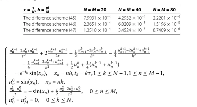
Table 1 Error analysis
τ=1N,h =piM N = M = 20 N = M = 40 N = M = 80 The difference scheme (45) 7.9931×10⁻⁴ 4.2932×10⁻⁴ 2.2201×10⁻⁴
The difference scheme (46) 2.3651×10⁻⁴ 6.0209×10⁻⁵ 1.5196×10⁻⁵
The difference scheme (47) 1.3510×10⁻⁴ 3.4524×10⁻⁵ 8.7409×10⁻⁶
⎧ ⎪ ⎪ ⎪ ⎪ ⎪ ⎪ ⎪ ⎪ ⎪ ⎪ ⎨ ⎪ ⎪ ⎪ ⎪ ⎪ ⎪ ⎪ ⎪ ⎪ ⎪ ⎩
uk+
n –ukn+ukn–
τ +
uk+
n –ukn– τ –
uk
n+–ukn+ukn–
h –
uk+
n+–ukn++ukn+–
h
–u k–
n+–ukn–+ukn––
h +ukn+(ukn++ukn–)
=e–tksin(x
n), xn=nh,tk=kτ, ≤k≤N– , ≤n≤M– ,
u
n=sin(xn), xn=nh, un–un
τ = –sin(xn) + τ
un–un+un
τ , ≤n≤M,
uk=ukM= , ≤k≤N.
()
To solve these difference equations, a modified Gauss elimination method procedure is applied. Hence, we seek a solution of the matrix equation in the following form:
uj=αj+uj++βj+, uM= , j=M– , . . . , , ,
whereαj(j= , , . . . ,M) are (N+ )×(N+ ) square matrices, andβj(j= , , . . . ,M) are
(N+ )× column matrices defined by
αj+= –(B+Cαj)–A,
βj+= (B+Cαj)–(Dφ–Cβj), j= , , . . . ,M– ,
wherej= , , . . . ,M– ,α is the (N+ )×(N+ ) zero matrix, andβ is the (N+ )× zero matrix. The results of computer calculations show that the second-order difference schemes are more accurate than the difference scheme of the first order of accuracy. Table is constructed forN=M= , , and , respectively.
The errors are computed by
ENM= max
≤k≤N–,≤n≤M–
u(tk,xn) –ukn,
whereu(tk,xn) represents the exact solution anduknrepresents the numerical solution at
(tk,xn) and the results are given in Table .
5 Conclusion
abstract telegraph equations can be investigated. Of course, the stability estimates for the solution of the nonlocal boundary value problem have been established. The difference schemes of the first order and second order of accuracy for telegraph equations can be studied. The stability of the difference schemes has been established without any assump-tions as regards the grid steps.
Competing interests
The authors declare that they have no competing interests.
Authors’ contributions
All authors read and approved the final manuscript.
Author details
1Department of Mathematics, Fatih University, Istanbul, 34500, Turkey.2Department of Mathematics, Siirt University, Siirt,
56100, Turkey.
Acknowledgements
The authors are very grateful to the referees for their valuable and helpful comments, remarks, and suggestions.
Received: 19 November 2014 Accepted: 4 February 2015
References
1. Fattorini, HO: Second Order Linear Differential Equations in Banach Spaces. North-Holland, Amsterdam (1985) 2. Goldstein, JA: Semigroups of Linear Operators and Applications. Oxford Mathematical Monographs. Oxford
University Press, New York (1985)
3. Ashyralyev, A, Sobolevskii, PE: New Difference Schemes for Partial Differential Equations. Operator Theory: Advances and Applications. Birkhäuser, Basel (2004)
4. Ashyralyev, A, Sobolevskii, PE: Well-Posedness of Parabolic Difference Equations. Operator Theory: Advances and Applications. Birkhäuser, Basel (1994)
5. Ghorbanalizadeh, A, Sawano, Y: Approximation in Banach space by linear positive operators. Positivity18(3), 585-594 (2014)
6. Ashyralyev, A, Sobolevskii, PE: Two new approaches for construction of the high order of accuracy difference schemes for hyperbolic differential equations. Discrete Dyn. Nat. Soc.2005(2), 183-213 (2005)
7. De la Sen, M: On bounded strictly positive operators of closed range and some applications to asymptotic hyperstability of dynamic systems. Abstr. Appl. Anal.2013, Article ID 639576 (2013). doi:10.1155/2013/639576 8. De la Sen, M: Positivity and stability of the solutions of Caputo fractional linear time-invariant systems of any order
with internal point delays. Abstr. Appl. Anal.2011, Article ID 161246 (2011). doi:10.1155/2011/161246
9. Achour, D, Belacel, A: Domination and factorization theorems for positive stronglyp-summing operators. Positivity
18(4), 785-804 (2014)
10. Krein, SG: Linear Differential Equations in Banach Space. Translations of Mathematical Monographs, vol. 29. Am. Math. Soc., Providence (1971); Translated from the Russian by JM Danskin
11. Vasilev, VV, Krein, SG, Piskarev, S: Operator semigroups, cosine operator functions, and linear differential equations. In: Mathematical Analysis. Itogi Nauki i Tekhniki, vol. 28, pp. 87-202. Akad. Nauk SSSR Vsesoyuz. Inst. Nauchn. i Tekhn. Inform., Moscow (1990) (Russian); Translated in J. Soviet Math.54(4), 1042-1129 (1991)
12. Jordan, PM, Puri, A: Digital signal propagation in dispersive media. J. Appl. Phys.85(3), 1273-1282 (1999)
13. Weston, VH, He, S: Wave splitting of telegraph equation inR3and its applications to inverse scattering. Inverse Probl. 9, 789-812 (1993)
14. Banasiak, J, Mika, JR: Singularly perturbed telegraph equations with applications in the random walk theory. J. Appl. Math. Stoch. Anal.11(1), 9-28 (1998)
15. Dehghan, M, Shokri, A: A numerical methods for solving the hyperbolic telegraph equation. Numer. Methods Partial Differ. Equ.24(4), 1080-1093 (2008)
16. Gao, F, Chi, C: Unconditionally stable difference schemes for a one-space-dimensional linear hyperbolic equation. Appl. Math. Comput.187(2), 1272-1276 (2007)
17. Biazar, J, Ebrahimi, H, Ayati, Z: An approximation to the solution of telegraph equation by variational iteration method. Numer. Methods Partial Differ. Equ.25, 797-801 (2009)
18. Saadatmandi, A, Dehghan, M: Numerical solution of hyperbolic telegraph equation using the Chebyshev tau method. Numer. Methods Partial Differ. Equ.26(1), 239-252 (2010)
19. Koksal, ME: An operator-difference method for telegraph equations arising in transmission lines. Discrete Dyn. Nat. Soc.2011, Article ID 561015 (2011). doi:10.1155/2011/561015
20. Twizell, EH: An explicit difference method for the wave equation with extended stability range. BIT Numer. Math.
19(3), 378-383 (1979)
21. Ashyralyev, A, Akat, M: An approximation of stochastic hyperbolic equations. AIP Conf. Proc.1389, 625-628 (2011) 22. Ashyralyev, A, Akat, M: An approximation of stochastic hyperbolic equations: case with Wiener process. Math.
Methods Appl. Sci.36(9), 1095-1106 (2013)
23. Ashyralyev, A, Akat, M: An approximation of stochastic telegraph equations. AIP Conf. Proc.1479, 598-601 (2012) 24. Pogorelenko, V, Sobolevskii, PE: The ‘counter-example’ to W. Littman counter-example ofLp-energetical inequality for
wave equation. Funct. Differ. Equ.4(1-2), 165-172 (1997)
25. Kostin, VA: Analytic semigroups and cosine functions. Dokl. Akad. Nauk SSSR307(4), 796-799 (1989) (Russian) 26. Sobolevskii, PE: Difference Methods for the Approximate Solution of Differential Equations. Izdat. Voronezh. Gosud.