Global exponential stability and existence of periodic solutions for delayed reaction-diffusion BAM neural networks with Dirichlet boundary conditions

R E S E A R C H

Open Access

Global exponential stability and existence of

periodic solutions for delayed

reaction-diffusion BAM neural networks with

Dirichlet boundary conditions

Weiyuan Zhang

1*

_{, Junmin Li}

2

_{and Minglai Chen}

2

*_{Correspondence: [email protected]} 1_{Institute of Mathematics and}

Applied Mathematics, Xianyang Normal University, Xianyang, 712000, China

Full list of author information is available at the end of the article

Abstract

In this paper, both global exponential stability and periodic solutions are investigated for a class of delayed reaction-diffusion BAM neural networks with Dirichlet boundary conditions. By employing suitable Lyapunov functionals, sufficient conditions of the global exponential stability and the existence of periodic solutions are established for reaction-diffusion BAM neural networks with mixed time delays and Dirichlet boundary conditions. The derived criteria extend and improve previous results in the literature. A numerical example is given to show the effectiveness of the obtained results.

Keywords: neural networks; reaction-diffusion; mixed time delays; global exponential stability; Poincaré mapping; Lyapunov functional

1 Introduction

Neural networks (NNs) have been extensively studied in the past few years and have found many applications in different areas such as pattern recognition, associative memory, com-binatorial optimization,etc. Delayed versions of NNs were also proved to be important for solving certain classes of motion-related optimization problems. Various results concern-ing the dynamical behavior of NNs with delays have been reported durconcern-ing the last decade (see,e.g., [–]). Recently, the authors in [] and [] considered the problem of exponential passivity analysis for uncertain NNs with time-varying delays and passivity-based con-troller design for Hopfield NNs, respectively.

Since NNs related to bidirectional associative memory (BAM) were proposed by Kosko [], the BAM NNs have been one of the most interesting research topics and have attracted the attention of researchers. In the design and applications of networks, the stability of the designed BAM NNs is one of the most important issues (see,e.g., [–]). Many important results concerning mainly the existence and stability of equilibrium of BAM NNs have been obtained (see,e.g., [–]).

However, strictly speaking, diffusion effects cannot be avoided in the NNs when elec-trons are moving in asymmetric electromagnetic fields. So, we must consider that the ac-tivations vary in space as well as in time. In [–], the authors considered the stability of NNs with diffusion terms which were expressed by partial differential equations. In

ticular, the existence and attractivity of periodic solutions for non-autonomous reaction-diffusion Cohen-Grossberg NNs with discrete time delays were investigated in []. The authors derived sufficient conditions on the stability and periodic solutions of delayed reaction-diffusion NNs (RDNNs) with Neumann boundary conditions in [–]. In these works, due to the divergence theorem employed, a negative integral term with gradient was removed in their deduction. Therefore, the stability criteria acquired by them do not contain diffusion terms; that is to say, the diffusion terms do not have any effect on their deduction and results. Meanwhile, some conditions dependent on the diffusion coeffi-cients were given in [, –] to ensure the global exponential stability and periodicity of RDNNs with Dirichlet boundary conditions based on -norm.

To the best of our knowledge, there are few reports about global exponential stability and periodicity of RDNNs with mixed time delays and Dirichlet boundary conditions, which are very important in theories and applications and also are a very challenging problem. In this paper, by employing suitable Lyapunov functionals, we shall apply inequality tech-niques to establish global exponential stability criteria of the equilibrium and periodic solutions for RDNNs with mixed time delays and Dirichlet boundary conditions. The de-rived criteria extend and improve previous results in the literature [, ].

Throughout this paper, we need the following notations.Rn_{denotes then-dimensional}

Euclidean space. We denote

u(t,x) –u∗=

m

i=

ui–u∗i r

dx,

ϕu(s,x) –u∗= sup

–∞≤s≤

m

i=

ϕui(s,x) –u∗i r

dx

and

v(t,x) –v∗=

n

j=

_vj–v∗_jrdx,ϕv(s,x) –v∗= sup

–∞≤s≤

n

j=

ϕvj(s,x) –v∗j r

dx

,

r≥.

Letui=ui(t,x),vj=vj(t,x).

The remainder of this paper is organized as follows. In Section , the basic notations, model description and assumptions are introduced. In Sections  and , criteria are pro-posed to determine global exponential stability, and periodic solutions are considered for reaction-diffusion recurrent neural networks with mixed time delays, respectively. An il-lustrative example is given to illustrate the effectiveness of the obtained results in Sec-tion . We also conclude this paper in SecSec-tion .

2 Model description and preliminaries

In this paper, the RDNNs with mixed time delays are described as follows:

∂ui

∂t =

l

k= ∂ ∂xk

Dik

∂ui

∂xk

–pi

ui(t,x)

+

n

j=

bjifj

vj(t,x)

+

n

j= _˜

bji˜fj

vj

t–θji(t),x

+

n

j=

¯ bji

t

–∞kji(t–s)

¯ fj

vj(s,x)

ds+Ii(t),

∂vj

∂t =

l

k= ∂ ∂xk

D∗_jk∂vj

∂xk

–qj

vj(t,x)

()

+

m

i=

dijgi

ui(t,x)

+

m

i= _˜

dijg˜i

ui

t–τij(t),x

+

m

i=

¯ dij

t

–∞

¯

kij(t–s)g¯i

ui(s,x)

ds+Jj(t).

The RDNNs model given in () can be regarded as RDNNs with two layers, wheremis

the number of neurons in the first layer andnis the number of neurons in the second layer. x= (x,x, . . . ,xl)T∈⊂Rl,is a compact set with smooth boundary∂andmes> 

in the spaceRl_{;u= (u}

,u, . . . ,um)T∈Rm,v= (v,v, . . . ,vn)T∈Rn.ui(t,x) andvj(t,x)

rep-resent the state of theith neuron in the first layer and thejth neuron in the second layer at timetand in the spacex, respectively.bji,b˜ji,b¯ji,dij,d¯ijandd˜ijare known constants

denot-ing the synaptic connection strengths between the neurons in the two layers, respectively; fj,f˜j,f¯j,gi,g˜iandg¯idenote the activation functions of the neurons and the signal

propaga-tion funcpropaga-tions, respectively.IiandJjdenote the external inputs on theith neuron andjth

neuron, respectively;piandqjare differentiable real functions with positive derivatives

defining the neuron charging time;τij(t) andθji(t) represent continuous time-varying

de-lay and discrete dede-lay, respectively;Dik≥ andD∗jk≥,i= , , . . . ,m,k= , , . . . ,land

j= , , . . . ,n, stand for the transmission diffusion coefficient along theith neuron andjth neuron, respectively.

System () is supplemented with the following boundary conditions and initial values:

ui(t,x) = , vj(t,x) = , t≥,x∈∂, ()

ui(s,x) =ϕui(s,x), vj(s,x) =ϕvj(s,x), (s,x)∈(–∞, ]× ()

for anyi= , , . . . ,mandj= , , . . . ,n, wheren¯is the outer normal vector of∂,ϕ=ϕu

ϕv

= (ϕu, . . . ,ϕum,ϕv, . . . ,ϕvn)T ∈C are bounded and continuous, whereC=

ϕ|ϕ=ϕu

ϕv

,ϕ :

_{(–∞,]×R}m (–∞,]×Rn

→Rm+n_{. It is the Banach space of continuous functions which maps}(–∞,]

(–∞,]

intoRm+n_{with the topology of uniform convergence for the norm}

ϕ =

ϕu

ϕv

= sup

–∞≤s≤

m

i=

|ϕui|rdx

+ sup

–∞≤s≤

n

j=

|ϕvj|rdx

.

Remark  Some famous NN models became a special case of system (). For example, when Dik=  andD∗jk =  (i= , , . . . ,m,k= , , . . . ,l), the special case of model () is

the model which has been studied in [–]. Whenb˜ji=  andd˜ij= ,i= , , . . . ,m,j=

, , . . . ,n, system () became NNs with distributed delays and reaction-diffusion terms [, , ].

(A) The functionsτij(t), θji(t) are piecewise-continuous of classCon the closure of

each continuity subinterval and satisfy

≤τij(t)≤τij, ≤θji(t)≤θji, τ˙ij(t)≤μτ< , θ˙ji(t)≤μθ< ,

τ= max

≤i≤m,≤j≤n{τij}, θ=≤i≤maxm,≤j≤n{θji}

with some constantsτij≥,θji≥,τ> ,θ>  for allt≥.

(A) The functionspi(·) andqj(·) are piecewise-continuous of classCon the closure of

each continuity subinterval and satisfy

ai=inf

ζ∈Rp

i(ζ) > , pi() = ,

cj=inf

ζ∈Rq

j(ζ) > , qj() = .

(A) The activation functions and the signal propagation functions are bounded and Lipschitz continuous,i.e., there exist positive constantsLf_j,L˜f_j,Lf_j¯,Lg_i,Lg_i˜andL¯g_i such that for allη,η∈R,

fj(η) –fj(η)≤Lfj|η–η|, f˜j(η) –f˜j(η)≤L ˜

f

j|η–η|, f¯j(η) –f¯j(η)≤L

¯

f

j|η–η|, gi(η) –gi(η)≤Lig|η–η|, g_˜i(η) –g˜i(η)≤L˜

g

i|η–η|, g¯i(η) –g¯i(η)≤L¯ g

i|η–η|.

(A) The delay kernelsKji(s),K¯ij(s) : [,∞)→[,∞) (i= , , . . . ,m,j= , , . . . ,n) are

real-valued non-negative continuous functions that satisfy the following conditions:

(i) _+∞Kji(s)ds= ,

+∞

 K¯ji(s)ds= ;

(ii) _+∞sKji(s)ds<∞,

+∞

 sK¯ij(s)ds<∞;

(iii) There exist a positiveμsuch that

_+∞



seμsKji(s)ds<∞,

_+∞



seμsK¯ij(s)ds<∞.

Let (u∗,v∗) = (u∗_,u∗_, . . . ,u∗_n,v∗_,v∗_, . . . ,v∗_n) be the equilibrium point of system (). Definition  The equilibrium point of system () is said to be globally exponentially stable if we can findr≥ such that there exist constantsα>  andβ≥ such that

u(t,x) –u∗+v(t,x) –v∗ ≤βe–αt_ϕ

u(s,x) –u∗+ϕv(s,x) –v∗ ()

for allt≥.

Lemma [] Letbe a cube|xl|<dl(l= , . . . ,m),and let h(x)be a real-valued function

belonging to C_{()which vanishes on the boundary∂of,i.e.,h(x)|∂}

=.Then

h(x)dx≤d_l

_∂∂_xh_ldx. ()

3 Global exponential stability

Now we are in a position to investigate the global exponential stability of system (). By constructing a suitable Lyapunov functional, we arrive at the following conclusion.

Theorem  Let(A)-(A)be in force.If there exist wi>  (i= , , . . . ,n+m),r≥,γij> ,

βji> such that

wi

–rnar_i–Dil–rnari+ (r– ) n

j=

ar_i+ (r– )

n

j=

ar_iβ– r r–

ji

+

n

j=

wm+jmr

|dij|r

Lg_ir+|˜dij|r

eτ  –μτ

Lg_i˜r+|¯dij|rγijr

Lg_i¯r < 

and

wm+j

–rmcr_j–D∗_jl–rmcr_j+ (r– )

m

i=

cr_j+ (r– )

m

i=

cr_jγ– r r–

ij

+

m

i=

winr

|bji|r

Lf_jr+|˜bji|r

eθ  –μθ

Lf_j˜r+|¯bji|rβjir

L¯f_jr < , ()

in which i= , , . . . ,m,j= , , . . . ,n,Lf_j,Lf_j˜,L_jf¯,Lg_i,L_ig˜ and Lg_i¯ are Lipschitz constants,Di=

min≤k≤l{Dik/dk},D∗j =min≤k≤l{D∗jk/dk},then the equilibrium point(u∗,v∗)of system()is

unique and globally exponentially stable.

Proof If () holds, we can always choose a positive numberδ>  (may be very small) such that

wi

–rnar_i–Dil–rnari+ (r– ) n

j=

ar_i+ (r– )

n

j=

ar_iβ– r r–

ji

+

n

j=

wm+jmr

|dij|r

Lg_ir+|˜dij|r

eτ  –μτ

Lg_i˜r+|¯dij|rγijr

Lg¯i

i

r

+δ< 

and

wm+j

–rmcr_j–D∗_jl–rmcr_j+ (r– )

m

i=

cr_j+ (r– )

m

i=

cr_jγ– r r–

ij

+

m

i=

winr

|bji|r

Lf_jr+|˜bji|r

eθ  –μθ

Lf_j˜r+|¯bji|rβjir

L¯f_jr +δ< , ()

Let us consider the functions

Fi

x∗_i=wi

–rnar_i–Dil–rnari+ (r– ) n

j=

ar_i

+ (r– )

n

j=

ar_iβ– r r–

ji

+∞



kji(s)ds+ x∗inari–

+

n

j=

wm+jmr

|dij|r

Lg_ir+|˜dij|r

eτ  –μτ

Lg_i˜r

+|¯dij|rγijr

Lg¯i

i

r +∞



ex∗is_k¯

ij(s)ds

and

Gj

y∗_j=wm+j

–rmcr_j–D∗_jl–rmcr_j+ (r– )

m

i=

cr_j+ (r– )

m

i=

cr_jγ– r r–

ij

_+∞



¯ kij(s)ds

+ y∗_jmcr_j–

+

m

i=

winr

|bji|r

Lf_jr

+|˜bji|r

eθ  –μθ

Lf_j˜r+|¯bji|rβjir

Lf_j¯r

+∞



ey∗js_k

ji(s)ds , ()

wherex∗_i,y∗_j ∈[, +∞),i= , , . . . ,m,j= , , . . . ,n.

From () and (A), we deriveFi() < –δ< ,Gj() < –δ< ;Fi(x∗i) andGj(y∗j) are

con-tinuous forx∗_i,y∗_j ∈[, +∞). Moreover,Fi(x∗i)→+∞asx∗i →+∞andGj(y∗j)→+∞as

y∗_j →+∞. Thus there exist constantsεi,σj∈[, +∞) such that

Fi(εi) =wi

–rnar_i–Dil–rnari+ (r– ) n

j=

ar_i

+ (r– )

n

j=

ar_iβ– r r–

ji

+∞



kji(s)ds+ εinari–

+

n

j=

wm+jmr

|dij|r

Lg_ir

+|˜dij|r

eτ  –μτ

Lg_i˜r+|¯dij|rγijr

Lg¯i

i

r +∞



eεis_k¯

ij(s)ds = 

and

Gj(σj) =wm+j

–rmcr_j–D∗_jl–rmcr_j+ (r– )

m

i=

cr_j

+ (r– )

m

i=

cr_jγ– r r–

ij

+∞



¯

kij(s)ds+ σjmcrj–

+

m

i=

winr

|bji|r

Lf_jr

+|˜bji|r

eθ  –μθ

Lf_j˜r+|¯bji|rβjir

L¯f_jr

+∞



eσjs_k

ji(s)ds = , ()

By usingα=min_≤i≤m,≤j≤n{εi,σj}, obviously, we get

Fi(α) =wi

–rnar_i–Dil–rnari+ (r– ) n

j=

ar_i

+ (r– )

n

j=

ar_iβ– r r–

ji

+∞



kji(s)ds+ αnari–

+

n

j=

wm+jmr

|dij|r

Lg_ir

+|˜dij|r

eτ  –μτ

Lg_i˜r+|¯dij|rγijr

Lg¯i

i

r +∞



eαsk¯ij(s)ds ≤

and

Gj(α) =wm+j

–rmcr_j–D∗_jl–rmcr_j+ (r– )

m

i=

cr_j

+ (r– )

m

i=

cr_jγ– r r– ij _+∞  ¯

kij(s)ds+ αmcrj–

+

m

i=

winr

|bji|r

Lf_jr

+|˜bji|r

eθ  –μθ

Lf_j˜r+|¯bji|rβjir

Lf_j¯r

_+∞



eαskji(s)ds ≤, ()

wherei= , , . . . ,m,j= , , . . . ,n.

Suppose (u,v) = (u,u, . . . ,un,v,v, . . . ,vn)Tis any solution of model (). Rewrite model

() as

∂(ui–u∗i)

∂t =

l

k= ∂ ∂xk

Dik

∂(ui–u∗i)

∂xk

–pi

ui(t,x)

–pi

u∗_i

+ n j= bji fj

vj(t,x)

–fj

v∗_j+

n j= _˜ bji _˜ fj vj

t–θji(t),x

–f˜j

v∗_j

+ n j= ¯ bji t

–∞kji(t–s) _¯

fj

vj(s,x)

–f¯j

v∗_jds, ()

∂(vj–v∗j)

∂t =

l

k= ∂ ∂xk

D∗_jk∂(vj–v

∗

j)

∂xk

–qj

vj(t,x)

–qj

v∗_j

+ m i= dij gi

ui(t,x)

–gi

u∗_i+

m i= _˜ dij ˜ gi ui

t–τij(t),x

–g˜i

u∗_i

+ m i= ¯ dij t –∞ ¯ kij(t–s)

¯ gi

ui(s,x)

–g¯i

u∗_ids. ()

Multiplying () byui–u∗i and integrating overyield

  d dt

ui–u∗i

 dx = l k=

ui–u∗i

∂ ∂xk

Dik

∂(ui–u∗i)

∂xk

–p_i(ξi)

ui–u∗i

 dx+ n j= bji

ui–u∗i

fj(vj) –fj

v∗_jdx

+ n j= _˜ bji

ui–u∗i

_˜

fj

vj

t–θji(t),x

–f˜j

v∗_jdx

+ n j= ¯ bji

ui–u∗i t

–∞kji(t–s) _¯

fj

vj(s,x)

–¯fj

v∗_j ds

dx. ()

According to Green’s formula and the Dirichlet boundary condition, we get

l k=

ui–u∗i

∂ ∂xk

Dik

∂(ui–u∗i)

∂xk

dx= –

l k= Dik

∂(ui–u∗i)

∂xk



dx. ()

Moreover from Lemma , we have

– l k= Dik

∂(ui–u∗i)

∂xk



dx≤–

l k= Dik

d_k

ui–u∗i



dx≤–Dilui–u∗i



. ()

From ()-(), (A), (A) and the Holder integral inequality, we obtain that

d dt

ui–u∗i



dx

≤–Dil

ui–u∗i



dx– ai

ui–u∗i

 dx +  n j=

|bji|ui–u∗iL f

jvj–v∗jdx

+  n j=

|˜bji|ui–u∗if˜

vj

t–θji(t),x

–f˜v∗_jdx

+  n j=

|¯bji|

t

–∞kji(t–s)

ui–u∗if¯j

vj(s,x)

–f¯j

v∗_j ds

dx. ()

Multiplying both sides of () byvj–v∗j, similarly, we also have

d dt

vj–v∗j



dx

≤–D∗_jl

_vj–v∗_jdx– cj

_vj–v∗_jdx

+  m i=

|dij|Lgiui–u∗ivj–v∗jdx

+  m i=

|˜dij|g˜

ui

t–τij(t),x

–g˜u∗_ivj–v∗jdx

+  m i=

|¯dij|

t

–∞

¯

kij(t–s)g¯i

ui(s,x)

–g¯i

u∗_ivj–v∗jds

Choose a Lyapunov functional as follows:

V(t) =

m i= wi

nar_i–ui–u∗i r

eαt

+

n

j=

|˜bji|rnr

eθ  –μθ

t t–θji(t)

eαξ_f˜

j

vj(ξ,x)

–f˜j

v∗_jrdξ

+

n

j=

|¯bji|rnrβjir

_+∞



kji(s)

t t–s

eα(s+ξ)¯fj

vj(ξ,x)

–f¯j

v∗_jrdξds

dx + n j=

wm+j

mcr_j–vj–v∗j r

eαt

+

m

i=

|˜dij|rmr

eτ  –μτ

t t–τij(t)

eαξg˜i

ui(ξ,x)

–g˜i

u∗_irdξ

+

m

i=

|¯dij|rmrγijr

+∞



¯ kij(s)

t t–s

eα(s+ξ)g¯i

ui(ξ,x)

–g¯i

u∗_irdξds

dx.

Its upper Dini-derivative along the solution to system () can be calculated as follows:

D+V(t)≤

m i= wi

rnar_i–ui–u∗i

r–∂|ui–u∗i|

∂t e

αt_{+ αe}αt_nar–

i ui–u∗i r

+eαt

n

j=

|˜bji|rnr

eθ  –μθ

f˜j

vj(t,x)

–f˜j

v∗_jr

–

n

j=

|˜bji|rnr

eθ  –μθ

 –θ˙ji(t)

eα(t–θji(t))_f˜

j

vj

t–θji(t),x

–f˜j

v∗_jr

+eαt

n

j=

|¯bji|rnrβjir

+∞



eαskji(s)f¯j

vj(t,x)

–f¯j

v∗_jrds

–eαt

n

j=

|¯bji|rnrβjir

+∞



kji(s)f¯j

vj(t–s,x)

–f¯j

v∗_jrds

dx + n j=

wm+j

rmcr_j–vj–v∗j

r–∂|vj–v∗j|

∂t e

αt_{+ αe}αt_mcr–

j vj–v∗j r

+eαt

m

i=

|˜dij|rmr

eτ  –μτ

g_˜i

ui(t,x)

–g˜i

u∗_ir

–

m

i=

|˜dij|rmr

eτ  –μτ

eα(t–τij(t))_{( –τ}˙

ij)g˜i

ui

t–τij(t),x

–g˜i

u∗_ir

+eαt

m

i=

|¯dij|rmrγijr

+∞



eαsk¯ij(s)g¯i

ui(t,x)

–g¯i

u∗_irds

–eαt

m

i=

|¯dij|rmrγijr

_+∞



¯ kij(s)g¯i

ui(t–s,x)

–g¯i

u∗_irds

≤ m i= wi

rnar_i–ui–u∗i r–

eαt

–Dilui–u∗i



–aiui–u∗i

 + n j=

|bji|ui–u∗iL f

jvj–v∗j

+

n

j=

|˜bji|ui–u∗if˜

vj

t–θji(t),x

–f˜v∗_j

+

n

j=

|¯bji|

t

–∞kji(t–s)

ui–u∗if¯j

vj(s,x)

–f¯j

v∗_j ds

+ αeαt_nar–

i ui–u∗i r

+eαt n

j=

|˜bji|rnr

eθ  –μθ

f˜j

vj(t,x)

–f˜j

v∗_jr

–eαt n

j=

|˜bji|rnrf˜j

vj(t–θji,x)

–f˜j

v∗_jr

+eαt

n

j=

|¯bji|rnrβjir

+∞



eαskji(s)f¯j

vj(t,x)

–f¯j

v∗_jrds

–eαt

n

j=

|¯bji|rnrβjir

+∞



kji(s)f¯j

vj(t–s,x)

–f¯j

v∗_jrds

dx + n j=

wm+j

rmcr_j–vj–v∗j r–

eαt

–D∗_jlvj–v∗j



–cjvj–v∗j

 + m i=

|dij|L g

iui–u∗ivj–v∗j+ m

i=

|˜dij|g˜

ui(t–τij,x)

–g˜u∗_ivj–v∗j

+

m

i=

|¯dij|

t

–∞

¯

kij(t–s)g¯i

ui(s,x)

–g¯i

u∗_ivj–v∗j ds

+ αeαtmc_jr–vj–v∗j r

+eαt

m

i=

|˜dij|rmr

eτ  –μτ

g_˜i

ui(t,x)

–g˜i

u∗_ir

–eαt

m

i=

|˜dij|rmrg˜i

ui(t–τij,x)

–g˜i

u∗_ir

+eαt

m

i=

|¯dij|rmrγijr

+∞



eαsk¯ji(s)g¯i

ui(t,x)

–g¯i

u∗_irds

–eαt m

i=

|¯dij|rmrγijr

+∞



¯ kij(s)g¯i

ui(t–s,x)

–g¯i

u∗_irds

dx. ()

From () and the Young inequality, we can conclude

D+V(t)≤

eαt

m

i=

wi

–rnar_i–Dilui–u∗i r

–rnar_iui–u∗i r

+ (r– )

n

j=

+

n

j=

nr|bji|r

Lf_jrvj–v∗j r

+ (r– )

n

j=

ar_iui–u∗i r

+

n

j=

|˜bji|rnrf˜j

vj

t–θji(t),x

–f˜j

v∗_jr

+ (r– )

n

j=

ar_iβ– r r–

ji

t

–∞kji(t–s)

_ui–u∗_irds

+

n

j=

|¯bji|rnrβjir

t

–∞kji(t–s) f¯j

vj(s,x)

–f¯j

v_j∗rds + αna_ir–ui–u∗i r

+

n

j=

|˜bji|rnr

eθ  –μθ

f˜j

vj(t,x)

–f˜j

v∗_jr

–

n

j=

|˜bji|rnrf˜j

vj

t–θji(t),x

–f˜j

v∗_jr

+

n

j=

|¯bji|rnrβjir

+∞



eαskji(s)f¯j

vj(t,x)

–f¯j

v∗_jrds

–

n

j=

|¯bji|rnrβjir

+∞



kji(s)f¯j

vj(t–s,x)

–f¯j

v∗_jrds

dx

+

eαt

n

j=

wm+j

–rmcr_j–D∗_jlvj–v∗j r

–rmcr_jvj–v∗j r

+ (r– )

m

i=

cr_jvj–v∗j r + m i=

|dij|rmr

Lg_irui–u∗i r

+ (r– )

m

i=

cr_jvj–v∗j r

+

m

i=

|˜dij|rmrg˜i

ui

t–τij(t),x

–g˜i

u∗_ir

+ (r– )

m

i=

cr_jγ– r r– ij t –∞ ¯

kij(t–s)vj–v∗j r ds + m i=

|¯dij|rmrγijr

t

–∞

¯

kij(t–s)g¯i

ui(s,x)

–g¯i

u∗_irds

+ αmcr_j–vj–v∗j r

+

m

i=

|˜dij|rmr

eτ  –μτ

g_˜i

ui(t,x)

–g˜i

u∗_ir

–

m

i=

|˜dij|rmrg˜i

ui

t–τij(t),x

–g˜i

u∗_ir

+

m

i=

|¯dij|rmrγijr

+∞



eαsk¯ij(s)g¯i

ui(t,x)

–g¯i

u∗_irds

–

m

i=

|¯dij|rmrγijr

+∞



¯ kij(s)g¯i

ui(t–s,x)

–g¯i

u∗_irds

≤

eαt

m i= wi

–rnar_i–Dil–rnari+ (r– ) n

j=

ar_i+ αnar_i–

+ (r– )

n

j=

ar_iβ– r r–

ji

t

–∞kji(t–s)ds +

n

j=

wm+jmr

|dij|r

Lg_ir

+|˜dij|r

eτ  –μτ

Lg_i˜r+|¯dij|rγijr

+∞



eαsk¯ij(s)

Lg¯i

i

r

ds ui–u∗i r

dx

+

eαt

n

j=

wm+j

–rmcr_j–D∗_jl–rmcr_j+ (r– )

m

i=

cr_j

+ (r– )

m

i=

cr_jγ– r r– ij t –∞ ¯

kij(t–s)ds + αmcrj–

+

m

i=

winr

|bji|r

Lf_jr

+|˜bji|r

eθ  –μθ

L˜f_jr+|¯bji|rβjir

Lf_j¯r

+∞



eαskji(s)ds vj–v∗j r

dx. ()

From (), we can conclude

D+V(t)≤ and so V(t)≤V(), t≥. ()

Since

V() =

m i= wi

nar_i–ui(,x) –u∗i r

+

n

j=

|˜bji|rnr

eθ  –μθ



–θji(t) f˜j

vj(ξ,x)

–f˜j

v∗_jrdξ

+

n

j=

|¯bji|rnrβjir

+∞



kji(s)



–s

eα(s+ξ)_f¯

j

vj(ξ,x)

–f¯j

v∗_jrdξds

dx + n j=

wm+j

mcr_j–vj(,x) –v∗j r

+

m

i=

|˜dij|rmr

eτ  –μτ



–τij(t) g_˜i

ui(ξ,x)

–g˜i

u∗_irdξ

+

m

i=

|¯dij|rmrγijr

+∞



¯ kij(s)



–s

eα(s+ξ)_g¯

i

ui(ξ,x)

–g¯i

u∗_irdξds

dx ≤ m i= max ≤i≤m{wi}

nar_i–ui(,x) –u∗i r

+

n

j=

|˜bji|rnr

eθ  –μθ

L˜f_jr



–θji

vj(ξ,x) –v∗j r dξ + n j=

|¯bji|rnr

Lf_j¯rβ_jir +∞



kji(s)



–s

eα(s+ξ)vj(ξ,x) –v∗j r

dξds

+

n

j= max ≤j≤n{wm+j}

mcr_j–vj(,x) –v∗j r

+

m

i=

|˜dij|r

L˜g_irmr e τ

 –μτ



–τij

ui(ξ,x) –u∗i r

dξ

+

n

j=

|¯dij|rmr

Lg_i¯rγ_ijr +∞



¯ kji(s)



–s

eα(s+ξ)ui(ξ,x) –u∗i r

dξds

dx

≤

max

≤i≤m{wi}+≤maxj≤n{wm+j}≤maxj≤n

_m

i=

|¯dij|rmr

L¯g_irγ_ijr +∞



¯

kij(s)seαsds

+max

≤j≤n{wm+j}≤maxj≤n

_m

i=

|˜dij|r

L˜g_irmr e τ_τ

 –μτ

ϕu(s,x) –u∗ r

+

max

≤j≤n{wm+j}+≤maxi≤m{wi}≤maxi≤m

_n

j=

|¯bji|rnr

Lf_j¯rβ_jir _+∞



seαskji(s)ds

+max

≤i≤m{wi}≤maxi≤m

_n

j=

|˜bji|rnr

Lg_j˜r e θ_θ

 –μθ

ϕv(s,x) –v∗ r

. ()

Noting that

eαt

min ≤i≤m+nwi

u(t,x) –u∗+v(t,x) –v∗≤V(t), t≥. ()

Let

β=max

max

≤i≤m{wi}+≤maxj≤n{wm+j}≤maxj≤n

_m

i=

|¯dij|rmr

Lg_i¯rγ_ijr +∞



¯

kij(s)seαsds

+max

≤j≤n{wm+j}≤maxj≤n

_m

i=

|˜dij|r

Lg_i˜rmr e τ_τ

 –μτ

,

max

≤j≤n{wm+j}+≤maxi≤m{wi}≤maxi≤m

_n

j=

|¯bji|rnr

L¯f_jrβ_jir +∞



seαskji(s)ds

+max

≤i≤m{wi}≤maxi≤m

_n

j=

|˜bji|rnr

Lg_j˜r e θ_θ

 –μθ

min ≤i≤m+n{wi}.

Clearly,β≥. It follows that

u(t,x) –u∗+v(t,x) –v∗≤βe–αtϕu(s,x) –u∗+ϕv(s,x) –v∗,

for anyt≥, whereβ≥ is a constant. This implies that the solution of () is globally

exponentially stable. This completes the proof of Theorem .

diffusion term. Obviously, Lyapunov functional to construct is more general and our re-sults expand the model in [, ].

Whenb˜ji=  andd˜ij=  (i= , , . . . ,m,j= , , . . . ,n), system () becomes the following

BAM NNs with distributed delays and reaction-diffusion terms:

∂ui

∂t =

l

k= ∂ ∂xk

Dik

∂ui

∂xk

–pi

ui(t,x)

+

n

j=

bjifj

vj(t,x)

+

n

j=

¯ bji

t

–∞kji(t–s)

¯ fj

vj(s,x)

ds+Ii(t),

∂vj

∂t =

l

k= ∂ ∂xk

D∗_jk∂vj

∂xk

–qj

vj(t,x)

+

m

i=

dijgi

ui(t,x)

+

m

i=

¯ dij

t

–∞

¯

kij(t–s)g¯i

ui(s,x)

ds+Jj(t).

()

For (), we get the following result.

Corollary  Let(A)-(A)be in force.If there exist wi>  (i= , , . . . ,n+m),r≥,γij> ,

βji> such that

wi

–rnar_i–Dil–rnari+ (r– ) n

j=

ar_i+ (r– )

n

j=

ar_iβ– r r–

ji

+

n

j=

wm+jmr

|dij|r

Lg_ir+|¯dij|rγijr

L¯g_ir< 

and

wm+j

–rmcr_j–D∗_jl–rmcr_j+ (r– )

m

i=

cr_j+ (r– )

m

i=

cr_jγ– r r–

ij

+

m

i=

winr

|bji|r

Lf_jr+|¯bji|rβjir

Lf_j¯r< , ()

where i= , , . . . ,m,j= , , . . . ,n,Lf_j,Lf_j˜,L_jf¯,Lg_i,Lg_i˜and L¯g_i are Lipschitz constants.Then the equilibrium point(u∗,v∗)of system()is unique and globally exponentially stable.

4 Periodic solutions

In this section, we consider the stability criterion for periodic oscillatory solutions of sys-tem (), in which external inputIi:R+→R,i= , , . . . ,m, andJj:R+→R,j= , , . . . ,n,

are continuously periodic functions with periodω, that is,

Ii(t+ω) =Ii(t), Jj(t+ω) =Jj(t), i= , , . . . ,m,j= , , . . . ,n.

Theorem  Let (A)-(A)be in force. There exists only oneω-periodic solution of sys-tem(),and all other solutions converge exponentially to it as t→+∞if there exist con-stants wi>  (i= , , . . . ,n+m),r≥,γij> ,βji>  (i= , , . . . ,m, j= , , . . . ,n)such

that

wi

–rnar_i–Dil–rnari+ (r– ) n

j=

ar_i+ (r– )

n

j=

ar_iβ– r r–

ji

+

n

j=

wm+jmr

|dij|r

Lg_ir+|˜dij|r

eτ  –μτ

Lg_i˜r+|¯dij|rγijr

Lg_i¯r < 

and

wm+j

–rmcr_j–D∗_jl–rmcr_j+ (r– )

m

i=

cr_j+ (r– )

m

i=

cr_jγ– r r–

ij

+

m

i=

winr

|bji|r

Lf_jr+|˜bji|r

eθ  –μθ

Lf_j˜r+|¯bji|rβjir

L¯f_jr < , ()

where i= , , . . . ,m and j= , , . . . ,n,Lf_j,L˜f_j,L_jf¯,Lg_i,L˜g_i and Lg_i¯ are Lipschitz constants in (A).

Proof For anyϕu

ϕv

,ψu

ψv

∈C, we denote the solutions of system () through_,ϕu

ϕv

and_,ψu

ψv

as

u(t,ϕu,x) =

u(t,ϕu,x), . . . ,um(t,ϕu,x)

T

, v(t,ϕv,x) =

v(t,ϕv,x), . . . ,vn(t,ϕv,x)

T

and

u(t,ψu,x) =

u(t,ψu,x), . . . ,um(t,ψu,x)

T

, v(t,ψv,x) =

v(t,ψv,x), . . . ,vn(t,ψv,x)

T

,

respectively. Define

ut(ϕu,x) =u(t+θ,ϕu,x), θ∈(–∞, ],t≥,

vt(ϕv,x) =v(t+θ,ϕv,x), θ∈(–∞, ],t≥.

Clearly, for anyt≥,ut(ϕu)

vt(ϕv)

∈C. Now, we define

yi=ui(t,ϕu,x) –ui(t,ψu,x), zj=vj(t,ϕv,x) –vj(t,ψv,x).

Thus, we can obtain from system () that

∂yi

∂t =

l

k= ∂ ∂xk

Dik

∂yi

∂xk

–pi

ui(t,ϕu,x)

–pi

ui(t,ψu,x)

+

n

j=

bji

fj

vj(t,ϕv,x)

–fj

vj(t,ψv,x)

+

n

j= _˜

bji

_˜

fj

vj

t–θji(t),ϕv,x

–f˜j

vj

t–θji(t),ψv,x

+

n

j=

¯ bji

t

–∞kji(t–s) _¯

fj

vj(s,ϕv,x)

–¯fj

vj(s,ψv,x) ds,

∂zj

∂t =

l

k= ∂ ∂xk

D∗_jk∂zj

∂xk

–qj

vj(t,ϕv,x)

–qj

vj(t,ψv,x)

+

m

i=

dij

gi

ui(t,ϕu,x)

–gi

ui(t,ψu,x)

+

m

i= _˜

dij

˜ gi

ui

t–τij(t),ϕu,x

–g˜i

ui

t–τij(t),ψu,x

+

m

i=

¯ dij

t

–∞

¯ kij(t–s)

¯ gi

ui(s,ϕu,x)

–g¯i

ui(s,ψu,x)

ds .

We consider the following Lyapunov functional:

V(t) =

m

i=

wi

nar_i–|yi|reαt

+

n

j=

|˜bji|rnr( –μθ)

t t–θji(t)

f˜j

vj(ξ,ϕv,x)

–f˜j

vj(ξ,ψv,x) r

dξ

+

n

j=

|¯bji|rnrβjir

+∞



kji(s)

t t–s

eα(s+ξ)

ׯfj

vj(ξ,ϕv,x)

–f¯j

vj(ξ,ψv,x)rdξds

dx

+

n

j=

wm+j

mcr_j–|zj|reαt

+

m

i=

|˜dij|rmr( –μτ)

t t–τij(t)

g_˜i

ui(ξ,ϕu,x)

–g˜i

ui(ξ,ψu,x) r

dξds

+

m

i=

|¯dij|rmrγijr

+∞



¯ kij(s)

t t–s

eα(s+ξ)

×g¯i

ui(ξ,ϕu,x)

–g¯i

ui(ξ,ψu,x)rdξds

dx.

By a minor modification of the proof of Theorem , we can easily get

u(t,ϕu,x) –u(t,ψu,x)+v(t,ϕv,x) –v(t,ψv,x)

≤βe–αt ϕu–ψu + ϕv–ψv

fort≥,in whichβ≥ is a constant. Now, we can choose a positive integerNsuch that

βe–αNω≤ 

, βe

–αNω_≤

. ()

Defining a Poincaré mappingP:C→Cby

P ϕu ϕv =

uω(ϕu)

vω(ϕv)

, ()

due to the periodicity of system, we have

PN ϕu ϕv =

uNω(ϕu)

vNω(ϕv)

. ()

Lett=Nω, then from ()-() we can derive that

PN

ϕu

ϕv

–PN

ψu ψv ≤   ϕu ϕv – ψu ψv ,

which shows thatPNis a contraction mapping. Therefore, there exists a unique fixed point

ϕu∗

ϕv∗

∈C, namely,PNϕu∗

ϕv∗

=ϕu∗

ϕv∗

.

SincePN_Pϕ_u∗ ϕv∗

=PPNϕ_u∗ ϕv∗

=Pϕu∗

ϕv∗

, thenPϕ∗u

ϕ∗v

is also a fixed point ofPN_{. Because of}

the uniqueness of a fixed point ofPN_{, thenP}ϕu∗

ϕv∗

=ϕu∗

ϕv∗

.

Let (u(t,ϕ_u∗,x),v(t,ϕ∗_v,x)) be the solution of system () through_,ϕu∗

ϕv∗

, then (u(t+

ω,ϕ_u∗,x),v(t+ω,ϕ∗_v,x)) is also a solution of system (). Clearly,

ut+ω

ϕ_u∗,x vt+ω

ϕ_v∗,x =

ut

uω

ϕ_u∗

vt

vω

ϕ∗_v =

ut

ϕ_u∗,x vt

ϕ_v∗,x fort≥. Hence (u(t+ω,ϕ∗_u,x),v(t+ω,ϕ∗_v,x))T_{= (u(t,ϕ}∗

u,x),v(t,ϕv∗,x))Tfort≥.

This shows that (u(t,ϕ_u∗,x),v(t,ϕ_v∗,x))Tis exactly oneω-periodic solution of system (), and it is easy to see that all other solutions of system () converge exponentially to it as

t→+∞. The proof is completed.

5 Illustration example

In this section, a numerical example is given to illustrate the effectiveness of the obtained results.

Example  Consider the following system on={(x,x)T| <xk<

√

.π,k= , } ⊂R:

∂ui

∂t =

l

k= ∂ ∂xk

Dik

∂ui

∂xk

–pi

ui(t,x)

+ n j=

bjifj

vj(t,x)

+ n j= _˜

bjif˜j

vj

t–θji(t),x

+ n j= ¯ bji t

–∞kji(t–s)

¯ fj

vj(s,x)

ds+Ii(t),

∂vj

∂t =

l

k= ∂ ∂xk

D∗_jk∂vj

∂xk

–qj

vj(t,x)

+ m i=

dijgi

ui(t,x)

+ m i= _˜

dijg˜i

ui

t–τij(t),x

+ m i= ¯ dij t –∞ ¯

kij(t–s)g¯i

ui(s,x)

ds+Jj(t),

Figure 1 The surface ofu1(x1, 0.5018,t) whenx2= 0.5018.

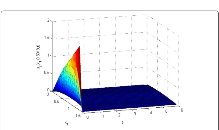
Figure 2 The surface ofu2(x1, 0.5018,t) whenx2= 0.5018.

ui= , vj= , t≥, x∈∂,

ui(s,x) =ϕui(s,x), vj(s,x) =ϕvj(s,x), (s,x)∈(–∞, ]×,

where kji(t) =k¯ij(t) =te–t,i,j,l= , .f(η) =f(η) =f˜(η) =f˜(η) =f¯(η) =¯f(η) =g(η) =

g(η) =g˜(η) =g˜(η) =g¯(η) =g¯(η) =tanh(η),n=m=l= ,λ= .,θji(t) =τij(t) = . –

.sin(πt),Lf_j =L_jf˜ =Lf_j¯ =Lg_i =L_ig˜ =L¯g_i = ,i,j= , . pi(ui(t,x)) =ui(t,x),qj(vj(t,x)) =

vj(t,x),D=D= ,D∗ =D∗= ,a=a= ,c=c= ,r= ,μτ =μθ= .,d= .,

d= ,d= .,d= .,d˜= –.,d˜= .,d˜= .,d˜= .,d¯= .,d¯= .,

¯

d= .,d¯= .,b= .,b= .,b= –.,b= –.,b˜= –,b˜= .,b˜= .,

˜