The Finite Element Sea Ice-Ocean Model (FESOM) v.1.4: formulation of an ocean general circulation model

(1)

Geosci. Model Dev., 7, 663–693, 2014 www.geosci-model-dev.net/7/663/2014/ doi:10.5194/gmd-7-663-2014

Geoscientific

Model Development

Open Access

The Finite Element Sea Ice-Ocean Model (FESOM) v.1.4:

formulation of an ocean general circulation model

Q. Wang, S. Danilov, D. Sidorenko, R. Timmermann, C. Wekerle, X. Wang, T. Jung, and J. Schröter

Alfred Wegener Institute for Polar and Marine Research, Bremerhaven, Germany

Correspondence to: Q. Wang (qiang.wang@awi.de)

Received: 10 June 2013 – Published in Geosci. Model Dev. Discuss.: 23 July 2013 Revised: 23 January 2014 – Accepted: 11 March 2014 – Published: 30 April 2014

Abstract. The Finite Element Sea Ice-Ocean Model (FE-SOM) is the first global ocean general circulation model based on unstructured-mesh methods that has been devel-oped for the purpose of climate research. The advantage of unstructured-mesh models is their flexible multi-resolution modelling functionality. In this study, an overview of the main features of FESOM will be given; based on sensitivity experiments a number of specific parameter choices will be explained; and directions of future developments will be out-lined. It is argued that FESOM is sufficiently mature to ex-plore the benefits of multi-resolution climate modelling and that its applications will provide information useful for the advancement of climate modelling on unstructured meshes.

1 Introduction

Climate models are becoming increasingly important to a wider range of users. They provide projections of anthro-pogenic climate change; they are extensively used for sub-seasonal, seasonal and decadal predictions; and they help us to understand the functioning of the climate system.

Despite substantial progress in climate modelling, even the most sophisticated models still show substantial short-comings. Simulations of the Atlantic meridional overturn-ing circulation, for example, still vary greatly in strength and pattern between climate models (Randall et al., 2007). Furthermore, many climate models still show substantial problems when it comes to simulating the observed path of the Gulf Stream. It is increasingly being recognized that a lack of sufficiently high spatial resolution is one of the main causes of the existing model shortcomings. In fact, many climate-relevant processes are too small scale in nature

to be explicitly resolved by state-of-the-art climate mod-els on available supercomputers and therefore need to be parametrized (Griffies, 2004; Shukla et al., 2009; Jakob, 2010).

In recent years a new generation of ocean models that em-ploy unstructured-mesh methods has emerged. These mod-els allow the use of high spatial resolution in dynami-cally active regions while keeping a relatively coarse res-olution otherwise. It is through this multi-resres-olution flexi-bility that unstructured-mesh models provide new opportu-nities to advance the field of climate modelling. Most ex-isting unstructured-mesh models have dealt with coastal or regional applications (e.g. Chen et al., 2003; Fringer et al., 2006; Zhang and Baptista, 2008).

This paper focuses on the setting of unstructured-mesh models for global applications, that is, on configurations more geared towards climate research applications. More specifically, the latest version of the Finite Element Sea Ice-Ocean Model (FESOM) – the first mature, global sea-ice ocean model that employs unstructured-mesh methods – will be described. The fact that FESOM solves the hydrostatic primitive equations for the ocean and comprises a finite ele-ment sea ice module makes it an ideal candidate for climate research applications. FESOM has been developed at the Al-fred Wegener Institute, Helmholtz Centre for Polar and Ma-rine Research (AWI) over the last 10 yr (Danilov et al., 2004; Wang et al., 2008; Timmermann et al., 2009).

(2)

664 Q. Wang et al.: The Finite Element Sea Ice-Ocean Model (FESOM)

Furthermore, the field is advancing so rapidly that details of the implementation of FESOM described in previous pa-pers (Danilov et al., 2004; Wang et al., 2008; Timmermann et al., 2009) are already outdated. It is also expected that other modelling groups working on the development of sim-ilar models (e.g. Ringler et al., 2013) will benefit from a de-tailed overview of our implementation of unstructured-mesh methods in global models. Finally, we expect that the present study, which also entails details on parametrizations and model tuning, will stimulate discussions and therefore ulti-mately advance the development of multi-resolution models. The basic numerical formulation of FESOM including spatial and temporal discretization is described in Sect. 2. Section 3 represents the key elements of FESOM which are fundamental in formulating ocean climate models. This sec-tion partly takes a review form, describing various physical parametrizations and numerical methods presented in the lit-erature. A short summary will be given in the last section. A brief historical review of FESOM’s development is given in the Appendix.

2 Numerical core of FESOM

2.1 Spatial discretization

Here we briefly explain the implementation of the finite ele-ment method in FESOM. For a detailed description of the im-plementation see Wang et al. (2008). The variational formu-lation with the FE method involves two basic steps. First, the partial differential equations (primitive equations) are mul-tiplied by a test function and integrated over the model do-main. Second, the unknown variables are approximated with a sum over a finite set of basis functions. FESOM uses the combination of continuous, piecewise linear basis functions in two dimensions for surface elevation and in three dimen-sions for velocity and tracers. For example, sea surface ele-vationηis discretized using basis functionsMi as

η'

M X

i=1

ηiMi, (1)

whereηi is the discrete value ofηat grid nodeiof the 2-D computational mesh. The test functions are the same as basis functions, leading to the standard Galerkin formulation.

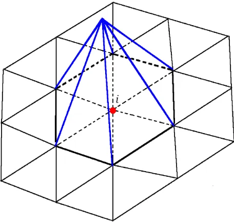
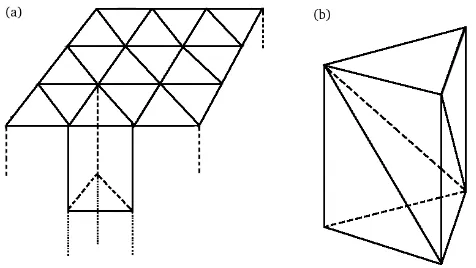
In two dimensions FESOM uses triangular surface meshes. Figure 1 shows the schematic of 2-D basis functions on a triangular mesh. The basis functionMiis equal to one at grid nodeiand goes linearly to zero at its neighbour nodes; it equals zero outside the stencil formed by the neighbour nodes. The 3-D mesh is generated by dropping vertical lines starting from the surface 2-D nodes, forming prisms which are then cut into tetrahedral elements (Fig. 2). Except for lay-ers adjacent to sloping ocean bottom each prism is cut into three tetrahedra; over a sloping bottom not all three tetra-hedra are used in order to employ shaved cells, in analogy to

Q. Wang et al.: The Finite Element Sea ice-Ocean Model (FESOM)

25

Fig. 11.

Schematic of horizontal discretization with the illustration

of basis functions used in FESOM. The

stencil

mentioned in the

text consists of seven nodes for node

i

in the example shown in this

figure.

Fig. 1. Schematic of horizontal discretization with the illustration of basis functions used in FESOM. The stencil mentioned in the text consists of seven nodes for nodeiin the example shown in this figure.

the shaved cells used by Adcroft et al. (1997). Keeping the 3-D grid nodes vertically aligned (i.e. all 3-3-D nodes have their corresponding 2-D surface nodes above them) is necessitated by the dominance of the hydrostatic balance in the ocean.

For a finite element discretization the basis functions for velocity and pressure (surface elevation in the hy-drostatic case) should meet the so-called LBB condition (Ladyzhenskaya, 1969; Babuska, 1973; Brezzi, 1974), oth-erwise spurious pressure modes can be excited. These modes are similar to the pressure modes of Arakawa A and B grids (Arakawa, 1966). The basis functions used in FESOM for velocity and pressure do not satisfy the LBB condition, so some measures to stabilize the code against spurious pres-sure modes are required. Note that prespres-sure modes on un-structured meshes are triggered more easily than in finite-difference models and robust stabilization is always needed.

(3)

Q. Wang et al.: The Finite Element Sea Ice-Ocean Model (FESOM) 665

26 Q. Wang et al.: The Finite Element Sea ice-Ocean Model (FESOM)

Fig. 12.Schematic of spatial discretization. The column under each surface triangle is cut to prisms(a), which can be divided to tetra-hedra(b). Except for layers adjacent to sloping ocean bottom each prism is cut to three tetrahedra.

Fig. 2. Schematic of spatial discretization. The column under each surface triangle is cut into prisms (a), which can be divided into tetrahedra (b). Except for layers adjacent to sloping ocean bottom each prism is cut into three tetrahedra.

horizontal velocity cannot be in the same functional space in the presence of bottom topography, leading to projection errors. The Appendix provides an overview on the develop-ment history of FESOM.

2.2 Temporal discretization

The advection term in the momentum equation is solved with the so-called characteristic Galerkin method (Zienkiewicz and Taylor, 2000), which is effectively the explicit second-order finite-element Taylor–Galerkin method. The method is based on taking temporal discretization using Taylor expan-sion before applying spatial discretization. Using this method with the linear spatial discretization as mentioned above, the leading-order error of the advection equation is still second order and generates numerical dispersion (Durran, 1999), thus requiring friction for numerical stability.

The horizontal viscosity is solved with the explicit Euler forward method (Sect. 3.9). The vertical viscosity is solved with the Euler backward method because the forward time stepping for vertical viscosity is unstable with a typical ver-tical resolution and time step.1To ensure solution efficiency, we solve the implicit vertical mixing operators separately from other parts of the momentum and tracer equations.2The surface elevation is solved implicitly to damp fast gravity

1_{The stability of an explicit Euler forward time stepping method}

for vertical viscosity requiresAv1t

1z2 ≤1/2, whereAvis the vertical

mixing coefficient. A typical time step of1t=40 min and a surface vertical resolution of1z=10 m requireAv≤0.02 m2s−1. Vertical

mixing coefficients in the surface boundary layer obtained from the KPP scheme (see Sect. 3.6) can readily be higher than this value locally.

2_{To guarantee global conservation the vertical diffusion}

equa-tions are solved using the finite element method. For continuous ba-sis functions the discretized vertical diffusion equations involve hor-izontal connections through the mass matrix with the time derivative term, and they cannot be solved efficiently. We chose to lump the matrix of time derivative terms (lumping means to sum all entries in

waves, and needs iterative solvers. The Coriolis force term uses the semi-implicit method to well represent inertial os-cillations.

The default tracer advection scheme is an explicit flux-corrected-transport (FCT) scheme (Sect. 3.5). The GM parametrization is incorporated into the model with the Eu-ler forward method (see Sect. 3.10 for the description of the GM parametrization), while the vertical diffusivity uses the Euler backward method for the same reason as for vertical viscosity.

An external iterative solver is called for solving the surface elevation equation. The final momentum and tracer equa-tions have only matrices of time derivative terms on the left-hand side of the equations, which can be relatively efficiently solved.3 Overall the dynamics and thermodynamics in the model are staggered in time with a half time step. That is, the new velocity is used to advect tracers, and the updated temperature and salinity are then used to calculate density.

2.3 Model efficiency

Models formulated on unstructured meshes are slower than their structured-mesh counterparts because of indirect mem-ory addressing and increased number of numerical oper-ations. If an unstructured-mesh model is ns times slower than typical structured-mesh models, simulations using it can computationally benefit from its unstructured-mesh func-tionality when the fine resolution region occupies less than 1/ns portion of the total computational area and most of the computational degrees of freedom are confined there. In the course of FESOM development we have chosen spatial and temporal discretization schemes by taking both model accu-racy and efficiency into account. FESOM is about 10 times slower than a typical structured-mesh model (Danilov et al., 2008). In its practical applications we therefore limit the lo-cally refined region to less than 10 % of the total domain area (e.g. Q. Wang et al., 2012; Timmermann et al., 2012; Timmermann and Hellmer, 2013; Wekerle et al., 2013; Wang et al., 2013). In these applications mesh resolutions are in-creased locally by factors ranging from 8 to 60 and most computational grid nodes are located inside the refinement region, ensuring great computational benefit.

The run-time memory access in the current FESOM ver-sion, hindered by its 1-D storage of variable arrays, is one of the bottlenecks for model efficiency. Some software engi-neering work is required in the future to identify the potential in improving memory access efficiency. Other unstructured-mesh numerical methods have shown potential in develop-ing more efficient ocean models (for a review see Danilov, 2013). In our model development team, we reserve some

a row to the diagonal in the matrix). This leads to a decoupled equa-tion for each water column, which can be very efficiently solved.

3_{Implicit advection and lateral friction would require iterative}

(4)

human resources for research on different numerical meth-ods, although currently the main effort is on FESOM devel-opment and its climate scale applications.

3 Key elements of the model

Different numerical and parametrization schemes are avail-able in FESOM. A detailed description of all the availavail-able features of FESOM is beyond the scope of the present study. Here the focus will be on those model elements that are cru-cial for climate scale applications. Illustrations of model sen-sitivity to different choices are presented here only for some of the model elements. A relatively complete description of the key model elements does not allow us to pursue thorough sensitivity studies for all of them here.

When configuring an OGCM for the purpose of climate research, choices for numerical and parametrization schemes are made according to the model developers’ practical ex-perience as well as knowledge from the literature. For the sake of the paper we provide a review form in some parts of the model description in this section. The review details the background for making our choices and importantly lists recommendations from previous studies which can improve model integrity. In our future work it will be valuable to eval-uate those recommended options that have not been tested with FESOM yet. We also note that the reviews made in this section are not complete in themselves as they are organized following our own model development issues considered so far. For a thorough review on ocean model fundamentals, see Griffies (2004).

All sensitivity tests presented in this section are based on atmospheric forcing fields taken from the inter-annual CORE-II data provided by Large and Yeager (2009). All sim-ulations were carried out for 60 yr over the period of forcing provided by Large and Yeager (2009).

3.1 Two-dimensional mesh

FESOM uses spherical coordinates, so the meridional and zonal velocities would be poorly approximated on a triangle covering the North Pole. To avoid the singularity a spher-ical coordinate system with the north pole over Greenland (40◦W, 75◦N) is used.4

FESOM uses triangular surface meshes. There are a few free triangle-mesh generators available, including DistMesh (Persson and Strang, 2004) and Triangle (Shewchuk, 1996). The mesh quality, the extent to which the triangles are close to equilateral ones, can be further improved after mesh gener-ation by relaxgener-ation of grid point locgener-ations. An abrupt change in resolution can lead to bad triangles (with too small/big in-ner angles and very different edge lengths) thus degrading the quality of meshes, so a transition zone between high and

4_{The three Euler angles for performing the rotation are (50}◦_, 15◦,−90◦) with thez–x–zrotation convention.

Q. Wang et al.: The Finite Element Sea ice-Ocean Model (FESOM) 27

Fig. 13.Horizontal resolution of an example mesh. This mesh is used in all simulations presented in this work.

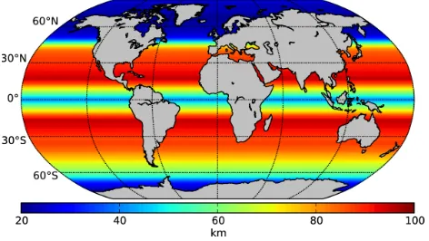
Fig. 3. Horizontal resolution of an example mesh. This mesh is used in all simulations presented in this work.

coarse resolutions is generally introduced. The resolution of a triangle is defined by its minimum height.

In practical applications with limited computational re-sources, we keep the horizontal mesh resolution coarse in most parts of the global ocean (for example, at nominal one degree as used in popular climate models), and refine par-ticularly chosen regions. The equatorial band with meridion-ally narrow currents and equatorimeridion-ally trapped waves requires higher resolution on the order of 1/3◦ (Latif et al., 1998; Schneider et al., 2003). Figure 3 shows the horizontal res-olution of an example mesh with increased resres-olution in the equatorial band. It is nominal one degree in most parts of the ocean and increases to 24 km poleward of 50◦N. The resolu-tion of this mesh is designed in terms of both kilometre (north of 50◦_{N) and geographical degree (south of 50}◦_{N) as a} par-ticular example, although it is not necessarily so in general cases. Thanks to the flexibility of unstructured meshes, one can fully avoid the imprint of geographic coordinates and de-sign meshes based on distances along the spherical surface.

(5)

It is worth mentioning that the model time step size is con-strained by the finest resolution on the mesh.5If the number of grid points in the high-resolution regions is only a few per-cent of the total grid points, we cannot enjoy the advantage of using FESOM because the overall time step size has to be set small. Therefore, in practice, increasing horizontal resolu-tion in narrow straits is usually implemented in applicaresolu-tions when some part of the ocean basin is also locally refined. In such applications a large portion of the computational grid points are in fine-resolution areas. To benefit from the multi-resolution capability even in cases when only a very small portion of the computational grid points have locally increased resolutions, multirate time stepping schemes are needed. Seny et al. (2013) gave an example of such schemes applied in a discontinuous Galerkin model.

3.2 Vertical coordinates and discretization

The choice of vertical coordinates or vertical grids is one of the most important aspects in the design of ocean cir-culation models (Griffies et al., 2000). Coordinated projects have been carried out to study the performance of different types of vertical discretization, – for example, DAMEE-NAB (Chassignet et al., 2000) and DYNAMO (Willebrand et al., 2001). Different vertical coordinates are used in ocean mod-els and each of them has its own advantages and disadvan-tages (Haidvogel and Beckmann, 1999; Griffies, 2004).

FESOM useszcoordinates (also called geopotential co-ordinates) in the vertical. The primitive equations are dis-cretized on z coordinates without coordinates transforma-tion, while sigma or more general vertical grids can be con-veniently used because of the FE formulation (Wang et al., 2008). The 2-D mesh and 3-D discretization (including grid types and vertical resolution) are set during the mesh gener-ation stage off-line before carrying out simulgener-ations.

Similar to traditional sigma grid models, truncation errors in computing hydrostatic pressure gradient exist on sigma grids in FESOM (see Sect. 3.4). The error in hydrostatic pres-sure gradient can be reduced by introducing high-order in-terpolations, but it is not trivial and can potentially degrade the solutions in climate scale simulations. Therefore,z-level grids are recommended in setting up ocean climate models. We use shaved cells over the ocean bottom onz-level grids to better represent the gentle topographic slopes (Adcroft et al., 1997; Wang et al., 2008). A faithful representation of bottom topography by using shaved (or partial) cells can generally improve the integrity of ocean model simulations (Maier-Reimer et al., 1993; Adcroft et al., 1997; Pacanowski and Gnanadesikan, 1998; Myers and Deacu, 2004; Barnier et al., 2006).

5_{While an implicit advection scheme is stable in terms of}

tempo-ral discretization, it is not necessarily accurate if the Courant num-ber (U 1t /1, whereUis the current speed,1tis the time step and

1is the grid spacing) is large.

Fig. 14.Horizontal resolution of an example mesh with the CAA region refined: (a)view in the stereographic projection and (b) zoomed to the CAA region.

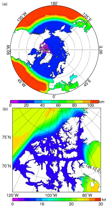
Fig. 4. Horizontal resolution of an example mesh with the CAA re-gion refined: (a) view in the stereographic projection and (b) close-up of the CAA region.

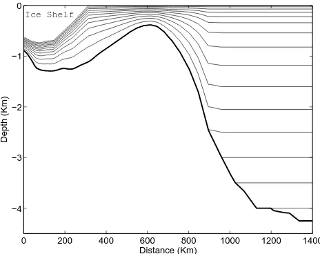
Combining zlevels in the bulk of the ocean with sigma grids in shelf regions of interest is a viable alternative toz -level grids. A schematic of such hybrid grids is shown in Fig. 5. These types of grids are used in FESOM when the ice cavities are included in the model (Timmermann et al., 2012). This hybrid grid is similar to the generalized coor-dinate used in POM (Princeton Ocean Model) described by Ezer and Mellor (2004). As illustrated in Fig. 5, sigma grids are used under ice shelf cavities and along the continental shelf around the Antarctic, while thez-level grids are used in all other parts of the global ocean to minimize pressure gradient errors.

(6)

Q. Wang et al.: The Finite Element Sea ice-Ocean Model (FESOM)

29

0 200 400 600 800 1000 1200 1400

−4 −3 −2 −1 0

Distance (Km)

Depth (Km)

Ice Shelf

Fig. 15.

Schematic of a hybrid vertical grids. The sigma grid is used

in adjunction with ice shelf modeling for the Antarctic region,

lo-cated under the ice shelf and along the continental shelf.

Z

-level

grids are used in other parts of the ocean.

Fig. 5. Schematic of a hybrid vertical grid. The sigma grid is used in adjunction with ice shelf modelling for the Antarctic region, located under the ice shelf and along the continental shelf;z-level grids are used in other parts of the ocean.

shelf and ocean basins exchange processes, including dense shelf water outflow and circumpolar water inflow; z-level grids with shaved cells under ice shelves are found to be use-ful in simulating the ocean circulation in ice cavities (Losch, 2008), while the merits of sigma grids are flexible vertical resolution and less grid scale noise, thus less spurious mix-ing.

On the z-level grid the vertical resolution is usually set finer in the upper 100–200 m depth to better resolve the sur-face boundary layer and becomes coarser with depth. Shaved cells are generally used at the bottom. In the region of sigma grids the vertical resolution is set depending on scientific in-terest, for example, increasing the near-surface resolution un-der the ice shelf and the near-bottom resolution where conti-nental shelf and basin water mass exchange is important. The vertical resolution distribution function of Song and Haidvo-gel (1994) is used in the mesh generator for adjusting the sigma grid resolution.6

6_{A convenient recipe is to define the sigma levels as}

z(k)=hmins(k)+(H−hmin){(1−θb)sinh(θ s(k))/sinh(θ )+

θb[tanh(θ (s(k)+0.5))−tanh(θ/2)]/(2tanh(θ/2))}, where k

(1≤k≤N) is the vertical layer index, hmin is the minimum

depth in the sigma grid region,H is the water column thickness,

s(k)= −(k−1)/(N−1)and N is the number of vertical layers (Song and Haidvogel, 1994). 0≤θ≤20 and 0≤θb≤1 are the

tuning parameters for designing the vertical discretization. Larger

θleads to more refined near-surface layers and ifθbapproaches 1

resolution at the bottom is also refined. A transition zone is required to smoothly connect the sigma andz-level grids.

3.3 Bottom topography

A blend of several bottom topography data sets is used to provide the bottom topography for FESOM. North of 69◦N the 2 km resolution version (version 2) of Interna-tional Bathymetric Chart of the Arctic Oceans (IBCAO ver-sion 2, Jakobsson et al., 2008) is used, while south of 64◦N the 1 min resolution version of General Bathymetric Chart of the Oceans (GEBCO) is used. Between 64◦N and 69◦N the topography is taken as a linear combination of the two data sets. The ocean bottom topography, lower ice surface height and ice shelf grounding line in the ice cavity regions around the Antarctica are derived from the one minute Re-fined Topography data set (Rtopo-1, Timmermann et al., 2010), which is based on the BEDMAP version 1 data set (Lythe et al., 2001).7

The raw topography data are used to determine the ocean coastlines. They are bilinearly interpolated to the model grid points. After the raw topography is interpolated to the model grid, grid scale smoothing of topography is applied to get rid of grid scale noise. The smoothing for each 2-D node is per-formed over its 2-D stencil (consisting of all 2-D nodes con-nected by edges with it).8Preliminary smoothing on coarse intermediate meshes should be avoided because it may be too strong for the fine part of the model mesh. One may choose to explicitly resolve narrow ocean straits using locally increased resolution in some cases and apply manual mesh and topog-raphy modification at unresolved straits in other cases. Mod-ellers need to decide how to treat individual narrow straits depending on the research interest and overall mesh design.

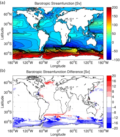
The topography is bilinearly interpolated from the data grid with fine resolution (2 km and 1 min) to model grids. If the model resolution is much lower than the topography data resolution, adequate smoothing of model topography can have a positive impact on the simulated ocean circula-tion. It is recommended to repeat the grid scale smoothing several times. Figures 6a and b show the bottom topography after applying stencil smoothing three and one times respec-tively for the coarse mesh shown in Fig. 3. Sensitivity exper-iments using these two versions of topography indicate that the former leads to a more realistic ocean circulation (Fig. 7). The barotropic stream functions with the two versions of model topography are different mainly in the Southern Ocean, along the western boundary and in the North Atlantic

7_{Improved ice bed, surface and thickness data sets for Antarctica}

(BEDMAP2, Fretwel et al., 2013) and a new bathymetry data set for the Arctic Ocean (IBCAO3, Jakobsson et al., 2012) have been released recently and their impact on model simulations compared to previous data sets need to be tested in sensitivity studies.

8_{The smoothing at node}_i _{is a weighted mean over its stencil.}

(7)

Fig. 16.Bottom topography(a)after three iterations of stencil filter and(b)after a single iteration.

Fig. 6. Bottom topography (a) after three iterations of stencil filter and (b) after a single iteration.

subpolar gyre. In the Weddell Sea, the maximum transport in observational estimates is 29.5 Sv along the transect be-tween the northern tip of the Antarctic Peninsula and Kapp Norvegia (Fahrbach et al., 1994) and more than 60 Sv at the Greenwich Meridian (Schroeder and Fahrbach, 1999). Ob-servations suggest mean southward transport at the Labrador Sea exit at 53◦N ranging from 37 Sv (Fischer et al., 2004) to 42 Sv (Fischer et al., 2010). Circulations in the South-ern Ocean and Labrador Sea are dynamically controlled by the Joint Effect of Baroclinicity and Relief (JEBAR, Olbers et al., 2004; Eden and Willebrand, 2001), so the model re-sults have large sensitivity to the treatment of bottom topog-raphy in these places. Because of the relatively coarse mesh (Fig. 3), maximum barotropic transport in these regions is weaker than observed in both simulations. The maximum gyre transport in Weddell Sea and North Atlantic subpolar gyre is about 34 Sv and 28 Sv respectively for the topogra-phy shown in Fig. 6a (see Fig. 7a). If topogratopogra-phy smoothing is applied only once, the transport is lower by about 10 Sv in both regions (see Fig. 7b).

Over the terrain-following part of the mesh the topogra-phy is smoothed by adjusting the slope parameterr0 (also

called Beckmann and Haidvogel number, Beckmann and Haidvogel, 1993) and the hydrostatic inconsistency number

Fig. 17. (a)Barotropic streamfunction (Sv) in a simulation with the topography of Fig. 16a and(b)its difference from a run with the topography of Fig. 16b. Shown are the mean values over the last 10yrof total 60yrsimulations.

Fig. 7. (a) Barotropic stream function (Sv) in a simulation with the topography of Fig. 6a and (b) its difference from a run with the topography of Fig. 6b. Shown are the mean values over the last 10 yr of total 60 yr simulations.

r1(also called Haney number, Haney, 1991).9The

smooth-ing helps to alleviate hydrostatic pressure gradient errors and maintain numerical stability. In practice we recommend the criteriar0≤0.2 andr1≤3. The smoothing is done on each

2-D stencil starting from the shallowest grid point until the deepest grid point. This procedure is repeated until the crite-ria are satisfied throughout the mesh.

3.4 Hydrostatic pressure gradient

Care should be taken in the calculation of the hydrostatic pressure gradient on sigma grids. Pressure gradient errors are not avoidable when the sigma grid surface deviates from the geopotential coordinate, but can be reduced with carefully designed numerics (Shchepetkin and McWilliams, 2003). A few measures are taken to reduce the errors in FE-SOM. The widely used method of exchanging the sequence

9_r

o and r1 are defined on edges between two neighbouring

nodes. r0=

|Hi−Hj|

Hi+Hj , where H is the water column thickness,

and subscripts i and j indicate two neighbouring nodes. r1=

zi(k)+zi(k+1)−zj(k)−zj(k+1)

zi(k)+zj(k)−zi(k+1)−zj(k+1), wherez(k)is the vertical coordinate

at layer k. The smoothing is done for r0 first and then for r1,

(8)

of integration and differentiation is employed (Song, 1998; Song and Wright, 1998). The horizontal derivatives of in situ density are taken first and pressure gradient forces are cal-culated then. In this way pressure gradient force errors are reduced but still present because of truncation errors in rep-resenting density with linear functions. The second measure is to use high-order interpolation in the vertical to interpolate density to a common depth for computing the density gradi-ent. The idea is discussed and assessed in Wang et al. (2008). In practice more measures are taken to control the pressure gradient errors on sigma grids. A common additional recipe is to apply topography smoothing to satisfy the criteria for

r0andr1as described in Sect. 3.3. Increasing resolution also

helps to reduce pressure gradient errors (Wang et al., 2008). Furthermore, the sigma grid as a part of the hybrid grid is only used around the Antarctic continental shelf and under ice shelves (Sect. 3.2), where we commonly use increased resolution to resolve small geometrical features.

3.5 Tracer advection

The commonly used tracer advection scheme in FESOM is an explicit second-order flux-corrected-transport (FCT) scheme. The classical FCT version described by Löhner et al. (1987) is employed as it works well for transient prob-lems. The FCT scheme preserves monotonicity and elimi-nates overshoots, a property useful for maintaining numerical stability on eddying scales. Upon comparison to a second-order scheme without flux limiter and an implicit second or-der scheme in idealized 2-D test cases, at coarse resolution the FCT scheme tends to slightly reduce local maxima even for a smooth field, but it well represents a sharp front and shows least dispersion errors in general (Wang, 2007).

Advection schemes should be able to provide adequate dissipation on grid scales and keep large scales less dissi-pated. Griffies and Hallberg (2000) show that it is impor-tant to adequately resolve the admitted scales of motion in order to maintain a small amount of spurious diapycnal mixing inz-coordinate models with commonly used advec-tion schemes. They find that spurious diapycnal mixing can reach more than 10−4m2s−1 depending on the advection scheme and the flow regime.10 Ilicak et al. (2012) demon-strate that spurious dianeutral transport is directly propor-tional to the lateral grid Reynolds number. Our preliminary tests show that the effective spurious diapycnal mixing as-sociated with the FESOM FCT scheme is similarly high as shown in Griffies and Hallberg (2000). Systematic research is needed for exploring alternative transport schemes and lim-iters and for investigating the dependence on the Reynolds number, especially in the context of mesh irregularity.

10_{The tests by Jochum (2009) indicate that relatively large}

spuri-ous mixing occurs locally in practice as varying background diffu-sivity at the order of 0.01×10−4m2s−1still produces difference in coarse model results.

3.6 Diapycnal mixing

Diapycnal mixing in the ocean has a strong impact on the dynamics of the ocean circulation and on the climate sys-tem as a whole (e.g. Bryan, 1987; Park and Bryan, 2000; Wunsch and Ferrari, 2004). The mixing processes are not re-solved in present ocean models and need to be parametrized. Thek-profile parametrization (KPP) proposed by Large et al. (1994) provides a framework accounting for important di-apycnal mixing processes, including wind stirring and buoy-ancy loss at the surface, non-local effects in the surface boundary layer, shear instability, internal wave breaking and double diffusion. Previous studies (Large et al., 1997; Gent et al., 1998) suggest that the KPP scheme is preferable in climate simulations. It is implemented in many current cli-mate models. It is also used in FESOM for large-scale simu-lations.11

Mixing induced by double diffusion (due to salt fingering and double diffusive convection) was found to have a rela-tively small impact on the mixed layer depth (Danabasoglu et al., 2006) and upper ocean temperature and salinity (Glessmer et al., 2008) in sensitivity studies, although its im-pact (mainly from salt fingering) on biogeochemical prop-erties is pronounced and cannot be neglected in ecosystem modelling (Glessmer et al., 2008). The double diffusion mix-ing scheme modified by Danabasoglu et al. (2006) is imple-mented in FESOM.

3.6.1 Diapycnal mixing from barotropic tides

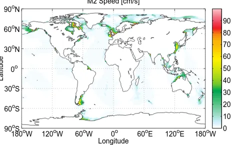
Mixing due to shear instability is parametrized as a function of Richardson number (Large et al., 1994). To include the mixing from barotropic tides interacting with ocean bottom, especially in the relatively shallow continental shelf regions, the tidal speed is accounted for in the computation of the Richardson number as proposed by Lee et al. (2006). As the tidal speed is large along the coast (Fig. 8), the Richardson number is small and vertical mixing is large in these regions. The original tidal mixing scheme of Lee et al. (2006) leads to too strong vertical mixing even far away vertically from the ocean bottom, as manifested by unrealistic winter polynyas in the central Weddell Sea in our simulations (not shown). The exponential decay as a function of distance from the ocean bottom suggested by Griffies (2012) is implemented in FESOM. It helps to remove the spurious large mixing.12

11_{Other mixing schemes are also used in climate models. For}

ex-ample, the current version of the MPIOM-ECHAM6 Earth System Model (Jungclaus et al., 2013) uses the Pacanowski and Philander (1981) scheme.

12_{The parametrization of mixing from barotropic tides}

inter-acting with the continental shelf is given by κ_vtidal=κmax(1+

σRi)−pexp−(H−|z|)/ztide_{, where} _κ_max=5×10−3m2s−1, σ=3,

p=1/4, Ri is the Richardson number based on tidal speed (see Lee et al., 2006, for details),His the water column thickness, and

(9)

180oW 120oW 60oW 0o 60oE 120oE 180oW 90oS

60oS 30oS 0o 30oN 60oN 90oN

Longitude

Latitude

M2 Speed [cm/s]

0 10 20 30 40 50 60 70 80 90

Fig. 18.M2 tidal speed map (cm s−1). High speed is mainly located in shallow shelf regions, including some Arctic and North Atlantic coastal regions.

Fig. 8. M2 tidal speed map (cm s−1). High speed is mainly located in shallow shelf regions, including some Arctic and North Atlantic coastal regions.

The barotropic tidal mixing was found to be useful as it assists in the horizontal spreading of river water at certain river mouths (Griffies et al., 2005). Our simulation shows that this is the case especially for the Arctic river runoff. The increased horizontal spreading of river water from the Arc-tic marginal seas leads to an increase in the freshwater flux at Fram Strait (see Fig. 9). The freshwater transport at Fram Strait shows the largest spread among the four Arctic gates in a recent Arctic Ocean model intercomparison, partly at-tributed to uncertainties in simulated salinity in the western Arctic Ocean (Jahn et al., 2012). Due to its impact on river water spreading and salinity, tidal mixing is among the key processes that need to be investigated to understand the re-ported model biases.

Mixing due to barotropic tides has a large-scale impact as it reduces the Atlantic Meridional Overturning Circula-tion (AMOC) (Fig. 10). The Labrador Sea Water producCircula-tion and AMOC are more sensitive to the freshwater exported through Fram Strait than through Davis Strait (Wekerle et al., 2013). The increased freshwater export through Fram Strait is an important mechanism through which tidal mixing can consequently weaken the Labrador Sea deep convection and AMOC, while there could be other relevant processes. It should be noticed that the tests shown here are carried out with an ocean-alone model and surface salinity restoring to climatology is enforced. Salinity restoring can provide a lo-cal salt sink/source. We speculate that the impact of tidal mixing on the Arctic freshwater export and large-scale cir-culation is also significant in coupled climate models (with-out surface salinity restoring). To include the impact of tides, Mueller et al. (2010) added a tidal model into a coupled cli-mate model (MPIOM-ECHAM5). In this case the tidal ve-locity is simulated and tidal mixing is explicitly taken into

times the M2 tide period). The exponential decay term was intro-duced by Griffies (2012) and does not exist in the original formula of Lee et al. (2006).

1950 1960 1970 1980 1990 2000

40 60 80 100 120

Years

Freshwater Transport (mSv)

Fram Strait Freshwater Transport

no tidal mixing with tidal mixing

Fig. 19.Time series of Fram Strait freshwater transport (m Sv−1). The impact of barotropic tidal mixing is illustrated.

Fig. 9. Time series of Fram Strait freshwater transport (m Sv−1). The impact of barotropic tidal mixing is illustrated.

account through the dependence of mixing coefficients on the Richardson number. They also reported that tides have pro-nounced influence on the ocean circulation, including weak-ening of the Labrador Sea deep convection.

3.6.2 Diapycnal mixing associated with internal wave energy dissipation

The background vertical diffusivity in the KPP scheme rep-resents the mixing due to internal wave breaking, which pro-vides mechanical energy to lift cold water across the ther-mocline and increase the potential energy of water, thus sus-taining the large-scale overturning circulation (Huang, 1999; Wunsch and Ferrari, 2004). Wind and tides are the main en-ergy sources for this mechanical enen-ergy in the abyss (Munk and Wunsch, 1998). Observational estimates indicate that the diapycnal diffusivity is of the order of 0.12±0.02−0.17±

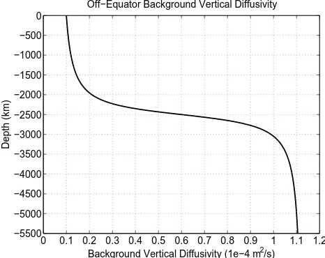
0.02×10−4m2s−1(Ledwell et al., 1993, 1998) in the sub-tropical Atlantic pycnocline and 0.15±0.07×10−4m2s−1 in the North Pacific Ocean (Kelley and Van Scoy, 1999), and much smaller values were observed near the equator (Gregg et al., 2003). In the deep ocean the diffusivity is observed to be small (0.1×10−4m2s−1) over smooth topography and much larger (1−5×10−4m2s−1) near the bottom in regions of rough topography (Polzin et al., 1997; Toole et al., 1997; Ledwell et al., 2000; Morris et al., 2001; Laurent et al., 2012). A modified version of the Bryan and Lewis (1979) back-ground vertical tracer diffusivity is used poleward of 15◦in the model formulation with FESOM (Fig. 11).13 The mini-mum value is 0.1×10−4_m2_s−1_{at the surface and the}

max-imum value is 1.1×10−4_m2_s−1_{close to the ocean bottom.}

Motivated by observations (Gregg et al., 2003) the magni-tude of this vertical profile is made one order smaller within the±5◦latitude range (0.01×10−4m2s−1at ocean surface) and increased linearly to the off-equator value at 15◦N/S. Using a coupled climate model Jochum et al. (2008) found

13_{The background vertical tracer diffusivity poleward of 15}◦_N/S is computed as a function of depth{0.6+1.0598/π×atan[4.5×

(10)

34 Q. Wang et al.: The Finite Element Sea ice-Ocean Model (FESOM)

Fig. 110. (a)

Atlantic Meridional Overturning Circulation (AMOC)

streamfunction (Sv) in a run without parameterized mixing due to

barotropic tides and

(b)

the difference from a run with the tidal

mix-ing. The results are the last 10

yr

mean in 60

yr

simulations.

Fig. 10. (a) Atlantic Meridional Overturning Circulation (AMOC) stream function (Sv) in a run without parametrized mixing due to barotropic tides and (b) the difference from a run with the tidal mix-ing. The results are the last 10 yr mean in 60 yr simulations.

that using the small background vertical diffusivity (0.01×

10−4m2s−1) in the equatorial band improves the tropical precipitation, although the improvement is only minor com-pared to existing biases. We use a constant background ver-tical viscosity of 10−4m2s−1, and there is no observational justification for this value.

Enhanced vertical mixing in the thermocline arising from Parametric Subharmonic Instability (PSI) of the M2 tide at the 28.9◦N/S band (Tian et al., 2006; Alford et al., 2007; Hibiya et al., 2007) is not accounted for in our model formu-lation. The model sensitivity study by Jochum et al. (2008) shows that increasing the off-equator background vertical diffusivity in the thermocline toward the observational esti-mate (0.17×10−4m2s−1instead of 0.1×10−4m2s−1) or ac-counting for the mixing arising from PSI worsens the North

Q. Wang et al.: The Finite Element Sea ice-Ocean Model (FESOM)

35

0 0.1 0.2 0.3 0.4 0.5 0.6 0.7 0.8 0.9 1 1.1 1.2

−5500 −5000 −4500 −4000 −3500 −3000 −2500 −2000 −1500 −1000 −500 0

Background Vertical Diffusivity (1e−4 m2/s)

Depth (km)

Off−Equator Background Vertical Diffusivity

Fig. 111.Fig. 11. Background vertical diffusivity poleward of 15Background vertical diffusivity poleward of 15◦N/S.◦N/S.

Atlantic results in their particular tests. Anyway, observa-tions for diapycnal diffusivity have motivated the utilization of more realistic diffusivity values in present climate models (see e.g. Danabasoglu et al., 2012).

The importance of the Arctic Ocean in the climate sys-tem especially in a warming world and the reported diffi-culty in robustly representing the surface and deep circu-lation in the Arctic Ocean in state-of-the-art ocean models (e.g. Karcher et al., 2007; Zhang and Steele, 2007; Jahn et al., 2012) warrant research on improving numerical mod-els including diapycnal mixing parametrizations. The diapy-cnal mixing in the halocline in the central Arctic Ocean is small compared to mid-latitude, largely due to the pres-ence of sea ice (Rainville and Winsor, 2008; Fer, 2009). The diapycnal diffusivity is 0.05±0.02×10−4m2s−1averaged over 70–220 m depth in the Amundsen Basin and as low as 0.01×10−4_m2_s−1_{in the upper cold halocline (Fer, 2009).}

A small background vertical diffusivity of 0.01×10−4_m2_s−1

was used in the KPP scheme and found to be optimal in some regional Arctic models (Zhang and Steele, 2007; Nguyen et al., 2009). The decrease in diapycnal diffusivity in the Arc-tic Ocean was taken into account in present climate models (e.g. Jochum et al., 2013). In our practice we found that us-ing this small value indeed improves the representation of the summer warm layer, but it increases the misfit of the halo-cline (too fresh in the upper halohalo-cline and too saline in the lower halocline in the model) and leads to too low freshwa-ter export through Fram Strait. Therefore, this local tuning of background diapycnal diffusivity for the Arctic Ocean is not adopted in FESOM. Presumably, using a more realistic vertical profile of diapycnal diffusivity with a range 0.01– 0.1×10−4_m2_s−1_{in the halocline as suggested by}

(11)

Improved understanding of mixing processes in the ocean has led to a parametrization of abyssal mixing induced by internal wave breaking associated with baroclinic tidal en-ergy (St Laurent et al., 2002; Simmons et al., 2004). Concen-trating intense mixing above rough topography where ma-jor tidal energy dissipates was found to be preferable for representing deep ocean stratification and Southern Ocean heat uptake in climate models (Saenko, 2006; Exarchou et al., 2013). The model sensitivity study by Jayne (2009) shows that using the tidal mixing parametrization proposed by St Laurent et al. (2002) can significantly enhance the deep cell of the meridional overturning circulation (MOC) in comparison with only using an ad hoc background ver-tical diffusivity, although the upper cell of the MOC and the poleward heat transport (the often used diagnostics for adjudging climate models) are not strongly affected by this parametrization. Present climate and earth system models tend to use the St Laurent et al. (2002) parametrization in-stead of the Bryan and Lewis (1979) type of background diffusivity (e.g. Danabasoglu et al., 2012; Delworth et al., 2012; Dunne et al., 2012). The merit of the abyssal diapy-cnal mixing parametrization of St Laurent et al. (2002) is that it is based on energy conservation and is more consis-tent with physical principles. Compared to the tidal mixing scheme by Lee et al. (2006) which tends to increase verti-cal diffusivity in regions of low Richardson numbers (par-ticularly the continental shelf regions), the parametrization of St Laurent et al. (2002) and Simmons et al. (2004) allows for enhanced tidal mixing in deep ocean regions. Comparing these different approaches remains for our future work.

Energy associated with mesoscale eddies is another im-portance source for turbulent mixing. Saenko et al. (2012) have recently investigated the individual effects of the tide and eddy dissipation energies on the ocean circulation. They showed that the overturning circulation and stratification in the deep ocean are too weak when only the tidal en-ergy maintains diapycnal mixing. With the addition of the eddy dissipation, the deep-ocean thermal structure became closer to that observed and the overturning and stratifica-tion in the abyss became stronger. Jochum et al. (2013) de-veloped a parametrization for wind-generated near-inertial waves (NIWs) and found that tropical sea surface tempera-ture and precipitation and mid-latitude westerlies are sensi-tive to the inclusion of NIW in their climate model. They concluded that because of its importance for global climate the uncertainty in the observed tropical NIW energy needs to be reduced. Presumably the recent progress in the under-standing of diapycnal mixing processes will increase model overall fidelity when practical parametrizations for these pro-cesses are taken into account.

3.7 Penetrative short-wave radiation

The infrared radiation from the solar heating is almost com-pletely absorbed in the upper 2 m water column, while the

ultraviolet and visible part of solar radiation (wavelengths

<750 nm) can penetrate deeper into the ocean depending on the ocean colour. In the biologically unproductive waters of the subtropical gyres, solar radiation can directly contribute to the heat content at depths greater than 100 m. Adding all the solar radiation to the uppermost cell in ocean models with a vertical resolution of 10 m or finer can overheat the ocean surface in regions where the penetration depth is deep in re-ality.

Many sensitivity studies have shown that adequately ac-counting for short-wave radiation penetration and its spacial and seasonal variation is important for simulating sea sur-face temperature (SST) and mixed layer depth at low latitude, equatorial undercurrents, and tropical cyclones and El Niño– Southern Oscillation (ENSO) (Schneider and Zhu, 1998; Nakamoto et al., 2001; Rochford et al., 2001; Murtugudde et al., 2002; Timmermann et al., 2002; Sweeney et al., 2005; Marzeion et al., 2005; Anderson et al., 2007; Ballabrera-Poy et al., 2007; Zhang et al., 2009; Jochum et al., 2010; Gnanadesikan et al., 2010; Liu et al., 2012). The solar radi-ation absorption is influenced by ocean colour on a global scale, so the bio-physical feedbacks have a global impact on the simulated results, including sea-ice thickness in the Arc-tic Ocean and the MOC (Lengaigne et al., 2009; Patara et al., 2012).

One traditional way to account for the spatial variation of short-wave penetration in climate models is to use spatially varying attenuation depths in an exponential penetration pro-file, which was found to be preferable compared to using a constant depth (Murtugudde et al., 2002). The seasonal variability of the attenuation depth plays an important role in the interannual variability in the tropical Pacific (Ballabrera-Poy et al., 2007). The interannual variability in short-wave absorption was also found to be important in representing ENSO in climate models (Jochum et al., 2010).

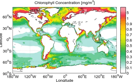
We use the short-wave penetration treatment as suggested by Sweeney et al. (2005) and Griffies et al. (2005). The op-tical model of Morel and Antoine (1994) is used to compute visible light absorption.14 The chlorophyll seasonal clima-tology of Sweeney et al. (2005) (see Fig. 12) is used in the computation. The visible light attenuation profile is obtained from the optical model, and the difference between two ver-tical grid levels is used to heat the cells in between. Sweeney et al. (2005) show that the optical models of Morel and An-toine (1994) and Ohlmann (2003) produce a relatively small difference in their ocean model.

14_{The attenuation profile of downward radiation in the}

vis-ible band is computed via IVIS(x, y, z)=I_VIS0 (x, y)(V1ez/ζ1+

V2ez/ζ2), whereV1,V2,ζ1andζ2are computed from an

(12)

180oW 120oW 60oW 0o 60oE 120oE 180oW 90oS

60oS 30oS 0o 30oN 60oN

Longitude

Latitude

Chlorophyll Concentration [mg/m3]

0 0.1 0.2 0.3 0.4 0.5 0.6 0.7 0.8 0.9 1 5

Fig. 112.Annual mean Chlorophyll concentration (mg m−3) clima-tology. Clear waters are mainly in the subtropical basins and high Chlorophyll concentration is seen in regions with high level of bio-logical activity. The data are from Sweeney et al. (2005).

Fig. 12. Annual mean chlorophyll concentration (mg m−3) clima-tology. Clear waters are mainly in the subtropical basins and high chlorophyll concentration is seen in regions with high level of bio-logical activity. The data are from Sweeney et al. (2005).

In some Earth System Models ecosystem models are used to better represent chlorophyll fields and the bio-physical feedbacks (Lengaigne et al., 2009; Loeptien et al., 2009; Jochum et al., 2010; Patara et al., 2012). Prognostic biogeo-chemistry is potentially beneficial in improving the fidelity of climate prediction through adaptive bio-physical feedbacks. An ecosystem model (REcoM, Schartau et al., 2007) has just been coupled to FESOM but is not included in the short-wave penetration parametrization in the present model version.

3.8 Vertical overturning

The hydrostatic approximation necessitates the use of a parametrization for unresolved vertical overturning pro-cesses. One approach is to use the convection adjustment schemes from Cox (1984) or Rahmstorf (1993). The latter scheme can efficiently remove all static instability in a water column. Another approach is to use a large vertical mixing coefficient (e.g. 10 m2s−1_{) to quickly mix vertically}

unsta-ble water columns and it is employed in FESOM.15As indi-cated by Klinger et al. (1996), using a large but finite vertical mixing coefficient can improve the simulation compared to instantaneous convection adjustment. Note that the vertical diffusion approach can only be realized through implicit time stepping.16

3.9 Horizontal viscosity

Horizontal momentum friction in ocean models is employed mainly for practical computational reasons and not motivated

15_{Super-parametrization as an alternative is found to be greatly}

superior to the convection adjustment parametrization at much less computational cost than running non-hydrostatic models (Campin et al., 2011). Its potential in climate modelling needs to be explored.

16_{Implicit time stepping methods for vertical diffusion are needed}

in general. See footnote 1.

by first principles (see the review of Griffies et al., 2000). As a numerical closure, horizontal friction is intended to sup-press grid noise associated with the grid Reynolds number and to resolve viscous boundary currents (Bryan et al., 1975; Large et al., 2001; Smith and McWilliams, 2003).17In prac-tice, horizontal friction in climate models is kept as small as feasible provided the grid noise is at an acceptable level and the western boundary layers are properly resolved.

Both Laplacian and biharmonic momentum friction op-erators are used in large-scale ocean simulations, and there is no first principle motivating either form. With respect to the dissipation scale-selectivity, the biharmonic operator is favourable compared to the Laplacian operator as it induces less dissipation at the resolved scales and concentrates dissi-pation at the grid scale (Griffies and Hallberg, 2000; Griffies, 2004). Large et al. (2001) and Smith and McWilliams (2003) proposed an anisotropic viscosity scheme by distinguishing the along and cross-flow directions in strong jets in order to reduce horizontal dissipation while satisfying the numerical constraints. Larger zonal viscosities were used in the equa-torial band to maintain numerical stability in the presence of strong zonal currents, and larger meridional viscosities were employed along the western boundaries to resolve the Munk boundary layer (Munk, 1950), while the meridional viscos-ity remained small in the equatorial band to better capture the magnitude and structure of the equatorial current. This approach was adopted in the previous GFDL climate model (Griffies et al., 2005), while isotropic viscosities are restored in a new GFDL Earth System Model to “allow more vigor-ous tropical instability wave activity at the expense of adding zonal grid noise, particularly in the tropics” (Dunne et al., 2012).

Different choices for viscosity values were made in dif-ferent ocean climate models. One choice is to use the pre-scribed viscosity. Due to the convergence of the meridians grid resolution also varies on structured meshes in some tra-ditional models. To avoid numerical instability associated with large viscosity in an explicit time stepping scheme, vis-cosity is often scaled with a power of the grid spacing (e.g. Bryan et al., 2007; Hecht et al., 2008). Another approach is to use flow-dependent Smagorinsky viscosities (Smagorinsky, 1963, 1993). The Smagorinsky viscosity is proportional to the local horizontal deformation rate times the squared grid spacing in the case of the Laplacian operator. It is enhanced in regions of large horizontal shear, thus providing increased

17_{In the case of Laplacian viscosity the grid Reynolds number}

is defined as Re =U 1/A, whereUis the speed of the currents,1

is the grid resolution, andAis the viscosity. In one dimension, the centred discretization of momentum advection requires Re<2 (or

A > U 1/2) to suppress the dispersion errors. The second constraint

A > (

√

(13)

dissipation where it is required to maintain stability. Its de-pendence on grid spacing eliminates the requirement for ad-ditional scaling as done for a priori specified viscosities.

We use the biharmonic friction with a Smagorinsky vis-cosity in FESOM large-scale simulations. Griffies and Hall-berg (2000) provide a thorough review on this scheme. As linear (first order) basis functions are used in FESOM, a direct formulation of the biharmonic operator cannot be achieved. Therefore, a two-step approach (first evaluating nodal Laplacian operators, then constructing the biharmonic operators) is used as described by Wang et al. (2008). The biharmonic Smagorinsky viscosity is computed as Laplacian Smagorinsky viscosity times12/8 as suggested from the lin-ear stability analysis (Griffies and Hallberg, 2000),18 where

1is the local grid resolution. The dimensionless scaling pa-rameter in the computation of Smagorinsky viscosity is set equal to π in our practice. To resolve the western bound-aries, a minimum biharmonic viscosity ofβ15is set at the four grid points close to the western boundaries, whereβ is the meridional gradient of the Coriolis parameter. When grid resolution is increased along the western boundaries and the velocity becomes more vigorous, the western boundary con-straint becomes less stringent than the Reynolds concon-straints (see the discussion in Griffies and Hallberg, 2000).

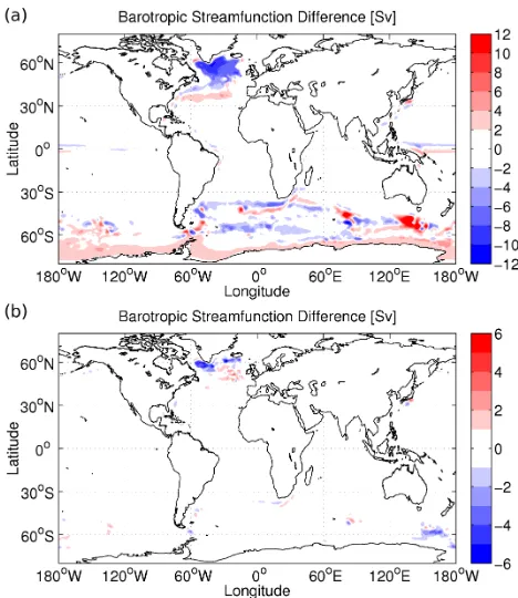
Figure 13a shows the sensitivity of barotropic stream func-tions to the two forms of friction operators (biharmonic and Laplacian). The Smagorinsky viscosity is used in both simu-lations. The difference of barotropic stream functions is seen mainly in the Southern Ocean and northern North Atlantic. In both regions the biharmonic viscosity leads to a stronger cir-culation, by about 4 Sv for the Antarctic Circumpolar Current (ACC) and 8 Sv for the subpolar gyre in the North Atlantic. Strong and narrow currents are sensitive to the form of fric-tion operators. The strength of North Atlantic Current, South Atlantic Current and Pacific equatorial current is enhanced by 2–4 Sv for the biharmonic case. Local impacts along ACC near topographic features or where the current narrows are also visible.

Consistent with the sensitivity study of Jochum et al. (2008), the boundary currents off east Greenland and west Greenland are enhanced with reduced momentum friction by using the biharmonic operator, thus increasing warm, saline Irminger Current water inflow to the Labrador Sea and de-creasing Labrador Sea sea-ice area (not shown).19Enhanced

18_{For centred differences in space and forward difference in time}

in a 2-D case, the stability requirement isA <₄1_1t2 for the Laplacian operator andB <₃₂1_1t4 for the biharmonic operator, thus a ratio of

12/8 betweenBandA, whereAis the Laplacian viscosity,Bis the biharmonic viscosity,1tis the time step and1is the horizontal resolution.

19_{Although a similar conclusion is obtained, our sensitivity tests}

are different from that of Jochum et al. (2008). They reduce mo-mentum dissipation by replacing the combination of background and Smagorinsky viscosity by only the background one, while we

Fig. 113. (a)Barotropic streamfunction difference (Sv) between runs with Laplacian and biharmonic Smagorinsky viscosities (the latter minus former).(b)The same as in(a)but between a run with biharmonic viscosity scaled with third power of the horizontal res-olution and a run with biharmonic Smagorinsky viscosity (the latter minus former). The results are the last 10yrmean in 60yr simula-tions.

Fig. 13. (a) Barotropic stream function difference (Sv) between runs with Laplacian and biharmonic Smagorinsky viscosities (the latter minus the former). (b) The same as in (a) but between a run with biharmonic viscosity scaled with third power of the horizontal res-olution and a run with biharmonic Smagorinsky viscosity (the latter minus the former). The results are the last 10 yr mean in 60 yr sim-ulations.

fraction of Atlantic Water in the Labrador Sea weakens the stratification and results in stronger deep convection there, thus an enhanced AMOC upper cell (by about 1 Sv, see Fig. 14a). The increase in subpolar gyre strength (Fig. 13a) is associated with increased density in the Labrador Sea re-sulting from enhanced Atlantic Water inflow and deep water ventilation.

More Atlantic Water accumulates south of the Greenland– Scotland Ridge (GSR) in the case of Laplacian friction, lead-ing to stronger deep convection north of 60◦N, which is man-ifested by the strengthening of the overturning circulation at intermediate depth between 50–60◦N (Fig. 14a). The com-monly called Labrador Sea Water feeding the Deep Western Boundary Current has its origin both in the Labrador Sea and south of GSR including the Irminger Sea (Pickart et al., 2003; Vage et al., 2008; de Jong et al., 2012). Deep mixed layers indicate the presence of deep convection in both regions in both simulations, but reduced dissipation in the biharmonic case favours it in the Labrador Sea. Since reduced dissipation drives both the AMOC and subpolar gyre strength toward

(14)

38 Q. Wang et al.: The Finite Element Sea ice-Ocean Model (FESOM)

Fig. 114.

Fig. 14. The same as Fig. 13 but for AMOC (Sv).

The same as Fig. 113 but for AMOC (Sv).

observations in our test, we choose to use the low dissipative biharmonic friction operator. Different regions of the global ocean were analysed in viscosity sensitivity experiments by Jochum et al. (2008), and generally improved ocean circula-tions were observed in their coupled climate model with re-duced dissipation (at the expense of an increase in numerical noise).

Figures 13b and 14b compare the impact of Smagorinsky and flow-independent, prescribed viscosities. In both sim-ulations the biharmonic friction is used. In the prescribed viscosity case, viscosity is a function of the cubed grid resolution,B013/13₀, where B0= −2.7×1013m4s−1 and

10=112 km. No obvious instability is visible in both

simu-lations. The difference in the large-scale circulation between the two simulations is clearly less significant than for the two friction operators. With the Smagorinsky viscosity the barotropic stream function is higher by 2–3 Sv in the cen-tral Labrador Sea. The increase in the AMOC upper cell is also rather small (0.1–0.2 Sv). The small difference between

the two simulations is not unexpected because the prescribed viscosity is relatively small.

Further evaluation of the impact of momentum dissipation on the large-scale circulation still needs to be pursued, es-pecially for eddy-permitting and eddy-resolving simulations. For example, an intermediate value of biharmonic viscosity (0.5B013/130) is found to produce good Gulf Stream

sep-aration and realistic North Atlantic Current penetration into the Northwest Corner region in eddy resolving (0.1◦) sim-ulations by Bryan et al. (2007). They got a southward dis-placed Gulf Stream separation with a lower viscosity and large SST errors at the subtropical–subpolar gyre boundary with a higher viscosity, indicating that only a small range in the parameter space exists for tuning their eddy-resolving model. To overcome the problems of too early separation of the Gulf Stream with a small biharmonic viscosity and es-tablishment of a permanent eddy north of Cape Hatters with a large biharmonic viscosity, Chassignet and Garraffo (2001) and Chassignet and Marshall (2008) recommend to jointly use biharmonic and Laplacian viscosity in eddy resolving models, with both values smaller than those when only one friction form is used. They found that by combining the two operators it is possible to retain the scale selectiveness of the biharmonic operator and to provide useful damping at larger scales, the latter of which helps to eliminate the wrong per-manent eddy. Some recent eddy permitting coupled climate models have chosen to use the biharmonic friction operator (Farneti et al., 2010; Delworth et al., 2012). Providing a uni-fied closure for momentum dissipation valid in various dy-namical situations and on meshes refined in different ways and in different regions remains an important and challeng-ing task in developchalleng-ing unstructured-mesh models.

In the sigma grid region in the case of using a hybrid grid, we apply momentum friction along the sigma grid slope to maintain numerical stability.20For unknown reasons the bi-harmonic operator turns out to be unstable even if it acts along the sigma grid slope. The two-step implementation of the biharmonic operator is presumably the cause of this prob-lem. Therefore we currently employ the Laplacian operator on sigma grids together with the Smagorinsky viscosity.

3.10 Eddy mixing and stirring

Much of the mixing induced by mesoscale eddies is oriented along locally referenced potential density surfaces (neutral surfaces, McDougall, 1987), which has motivated the uti-lization of rotated tracer diffusion (Redi, 1982; Olbers et al., 1985; Griffies et al., 1998).21The use of isoneutral diffusion

20_{As the sigma grid slope can be very steep, a horizontal friction}

imposes a large component perpendicular to the grid slope, which can readily lead to instability even with a very small time step in the case of a forward time stepping.

21_{Neutral diffusion is described by Laplacian operators in ocean}

(15)

numer-Q. Wang et al.: The Finite Element Sea Ice-Ocean Model (FESOM) 677

(often called Redi diffusion in the literature) significantly re-duces the unphysical diapycnal mixing associated with hor-izontal diffusion (Veronis, 1975; Böning et al., 1995), thus improving model integrity. In the bulk of the ocean interior the neutral slope is small, which motivates the application of the small slope approximation to simplify the diffusion ten-sor (Gent and McWilliams, 1990).

Gent and McWilliams (1990) and Gent et al. (1995) (re-ferred to as GM90 hereafter) provided a closure to repre-sent the adiabatic stirring effects of mesoscale eddies. They suggested a form of eddy-induced bolus velocity for z -coordinate models by considering the reduction of available potential energy through baroclinic instability. This bolus velocity is added in tracer equations to advect tracers to-gether with resolved velocity. The implementation of the GM parametrization in z-coordinates models significantly im-proves the model results including temperature distribution, heat transport and especially deep convection (Danabasoglu et al., 1994; Danabasoglu and McWilliams, 1995; Robitaille and Weaver, 1995; Duffy et al., 1995, 1997; England, 1995; England and Hirst, 1997; Hirst and McDougall, 1996, 1998; Hirst et al., 2000). The eddy-induced velocity as given by GM90 isv∗= −∂z(κgmS)+ ˆz∇ ·(κgmS), whereκgm is the

GM thickness diffusivity and S is the neutral slope. It in-volves computing the derivative of the thickness diffusivity and neutral slope and appears to be noisy in numerical real-izations, which is one of the factors that motivated the deriva-tion of the skew flux formuladeriva-tion for eddy-induced transport in Griffies (1998). Using the skew flux formulation also uni-fies the tracer mixing operators arising from Redi diffusion and GM stirring. It turns out to be very convenient in its im-plementation in the variational formulation in FESOM. Over-all, the small slope approximation for neutral diffusion (Gent and McWilliams, 1990) and the skew diffusion form for eddy stirring (Griffies et al., 1998) are the standard neutral physics options in FESOM.

In FESOM there is a caveat with hybrid grids, for which the sigma grid is used around the Antarctic coast when ice shelf cavities are present. Because sigma grid slopes and neutral slopes are very different, using neutral physics parametrization will lead to numerical instability on sigma grids. For the moment we use along-sigma diffusivity. The roles played by mesoscale eddies on continental shelf and in ice cavities around the Antarctic are unclear. In practice we use high resolution (∼10 km or finer) in the sigma grid re-gion, which can eliminate the drawback to some extent.

3.10.1 Diabatic boundary layer

Neutral diffusion represents mesoscale mixing in the adia-batic ocean interior. In the surface diaadia-batic boundary layer where eddies reaching the ocean surface are kinematically

ical stability (Roberts and Marshall, 1998). Griffies (2004) provides a thorough review on the properties of biharmonic operators and ex-plains why Laplacian operators are preferable for tracer diffusion.

constrained to transport horizontally, horizontal diffusion is more physical and should be applied (Treguier et al., 1997). This idea has been commonly taken in ocean cli-mate model practice (e.g. Griffies, 2004; Griffies et al., 2005; Danabasoglu et al., 2008). We use the mixed layer depth (MLD) as an approximation of the surface diabatic bound-ary layer depth, within which horizontal diffusion is applied. The MLD is defined as the shallowest depth where the inter-polated buoyancy gradient matches the maximum buoyancy gradient between the surface and any discrete depth within that water column (Large et al., 1997).

The diffusion tensor is not bounded as the neutral slopes increase, so numerical instability can be incurred when the neutral slopes are very steep. Therefore, the exponential ta-pering function suggested by Danabasoglu and McWilliams (1995) is applied to the diffusion tensor to change neutral diffusion to horizontal diffusion in regions of steep neutral slopes.22 The same tapering function is also applied to the GM thickness diffusivityκgmbelow the MLD to avoid

un-bounded eddy velocityv∗, which is proportional to the gra-dient of neutral slopes.

Within the surface boundary layer we treat the skew flux as implemented by Griffies et al. (2005). The product(κgmS)

is linearly tapered from the value at the base of the surface boundary layer to zero at the ocean surface, as suggested by Treguier et al. (1997). A linear function ofκgmSwith depth

means that the horizontal eddy velocityu∗_{= −}_∂

z(κgmS)is

vertically constant in the surface boundary layer. Maintaining an eddy-induced transport in the boundary layer is supported by the fact that baroclinic eddies are active in deep convec-tion regions (see the review by Griffies, 2004). Indeed, sim-ulations parametrizing eddy-induced velocity in the surface boundary layer show significant improvements compared to a control integration that tapers the effects of the eddies as the surface is approached (Danabasoglu et al., 2008). Our imple-mentation of the GM eddy flux near the surface is different from that of Griffies et al. (2005) with respect to the defi-nition of the boundary layer. We define the surface diabatic boundary layer depth using the MLD definition of Large et al. (1997), while the boundary layer base is set to where the magnitude of the slopeSin either horizontal direction is just greater than a critical value in Griffies et al. (2005).

Using the MLD to define the surface diabatic layer elim-inates the requirement to choose a critical neutral slope for defining the boundary layer. Additionally, tests with FESOM show that boundary layer depth fields defined via critical neutral slopes are less smooth than MLD, which is possibly

22_{The tapering function is only applied to the off-diagonal}

en-tries of the diffusion tensor, thus maintaining a horizontal diffu-sion when these entries are tapered to zero. The function sug-gested by Danabasoglu and McWilliams (1995) isf (S)=0.5(1+

tanh(Smax−|S|

Sd )), whereSd=0.001 is the width scale of the

taper-ing function andSmax=0.05 is the cut-off value beyond whichf